

Enhanced Link Prediction and Traffic Load Balancing in Unmanned Aerial Vehicle-Based Cloud-Edge-Local Networks


Abstract
:1. Introduction
- We propose a UAV-based elastic scheduling architecture for cloud-edge-local network resources, effectively utilizing UAV flexibility to enhance network deployment and employing the fat-tree topology structure to improve network scalability and management efficiency.
- We introduce the GA–GLU graph representation learning method to predict UAV links, accurately forecasting UAV network topology changes for dynamic resource scheduling.
- We propose the FERL-LB algorithm, which integrates reinforcement learning to optimize traffic load balancing based on link prediction, significantly improving network performance and resource utilization.
2. Related Works
2.1. UAV-Based Cloud-Edge-Local Resource Scheduling
2.2. UAV Link Topology Prediction
2.3. Traffic Load Balancing in Cloud-Edge-Local Networks
3. Methodology
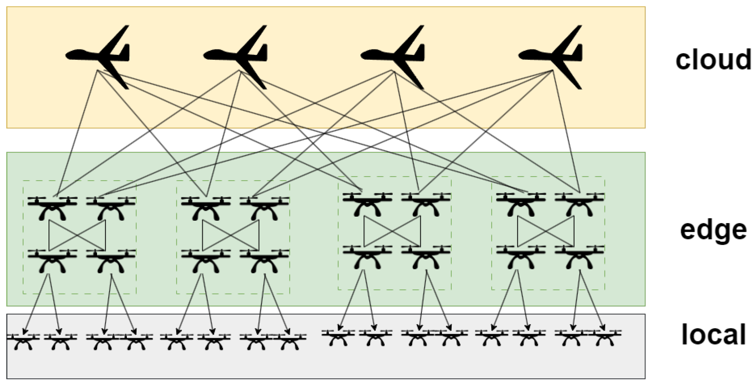
3.1. Design of Cloud-Edge-Local Architecture
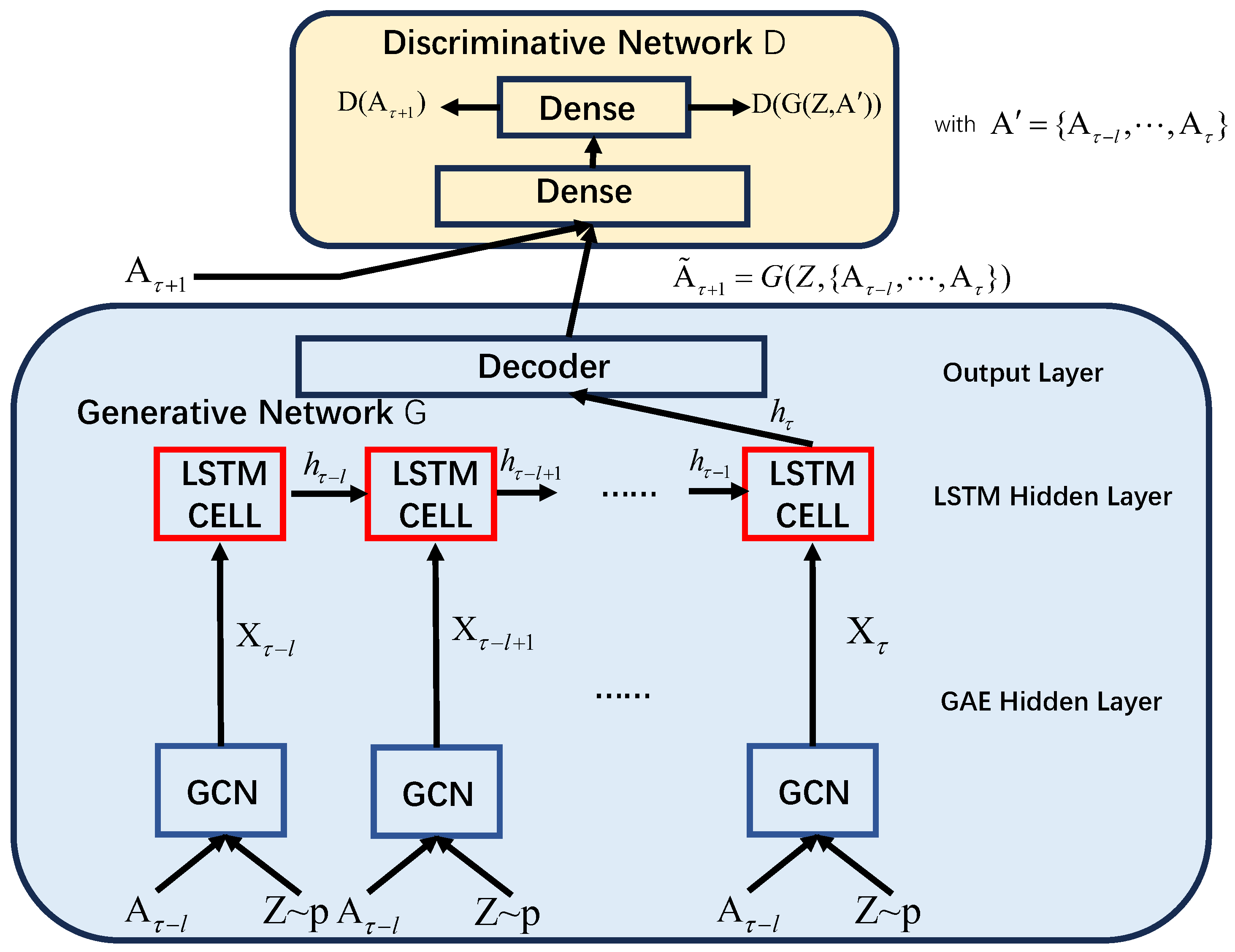
3.2. GA–GLU Link Prediction
3.2.1. Architecture
| Algorithm 1 GA–GLU Prediction Algorithm | |
| Input: Graph snapshots | |
| Output: Predicted future graph snapshot | |
| 1: // Initialize GAE and LSTM networks | |
| 2: Initialize GAE encoder and decoder | |
| 3: Initialize LSTM network | |
| 4: Initialize GAN generator G and discriminator D | |
| 5: // Process each graph snapshot | |
| 6: for to T do | |
| 7: | ▹ Encode the current graph snapshot |
| 8: | ▹ Decode to reconstruct the graph |
| 9: Feed into | ▹ Input to LSTM to update hidden state |
| 10: end for | |
| 11: // Use LSTM’s output to predict the next state | |
| 12: | |
| 13: | ▹ Decode to predict the next graph snapshot |
| 14: // Train GAN | |
| 15: repeat | |
| 16: Sample mini-batch of real snapshots | |
| 17: Generate fake snapshots from G | |
| 18: Train discriminator D to distinguish real from fake | |
| 19: Train generator G to fool D | |
| 20: until convergence | |
| 21: return | ▹ Return the predicted future graph snapshot |
3.2.2. GAE Layer
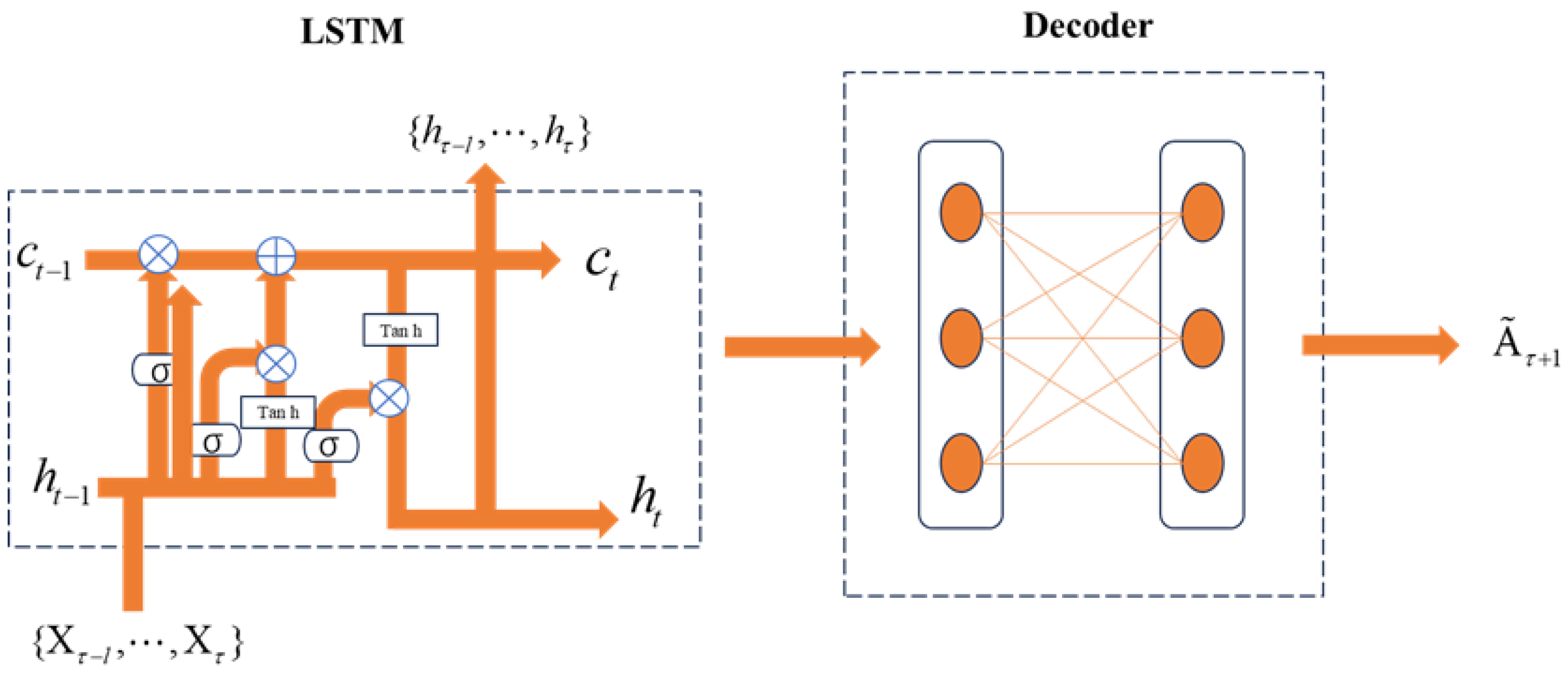
3.2.3. LSTM Layer
3.2.4. GAN Layer
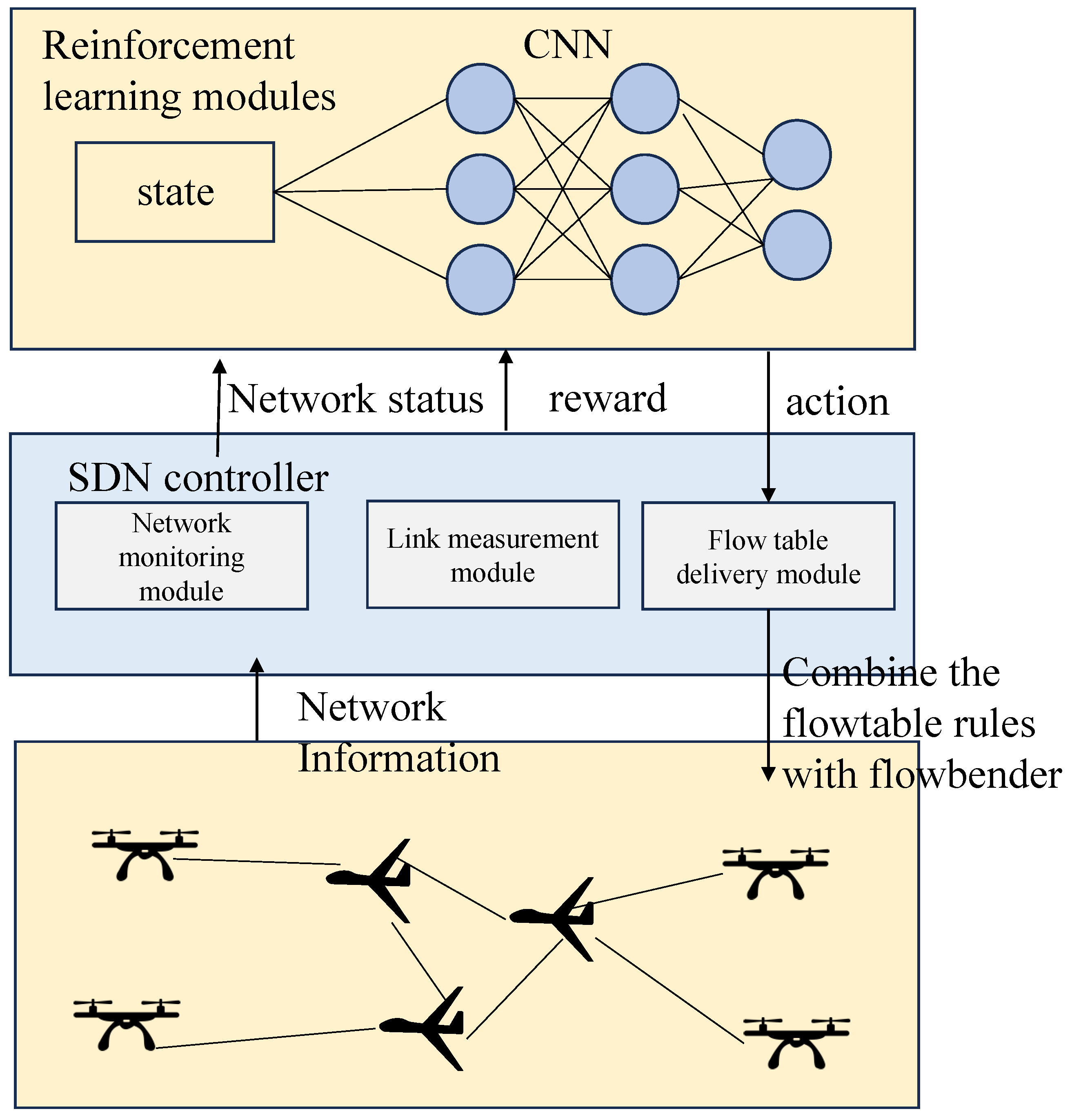
3.3. FERL-LB Algorithm
3.3.1. Architecture
| Algorithm 2 FERL-LB Algorithm Using DDQN |
|
3.3.2. Deep Q-Networks and Double Q-Learning
3.3.3. Traffic Forwarding Design
4. Experiment
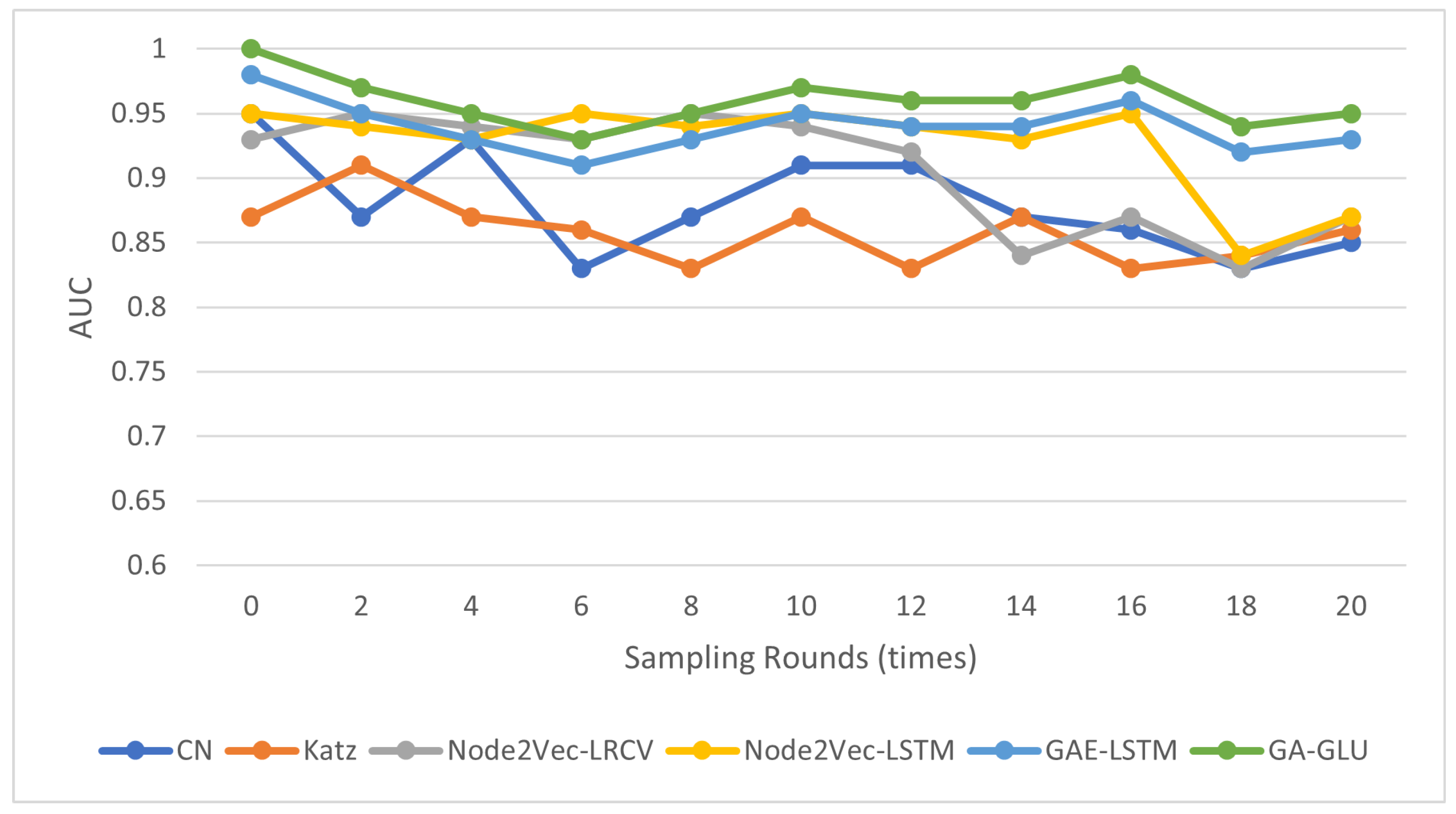
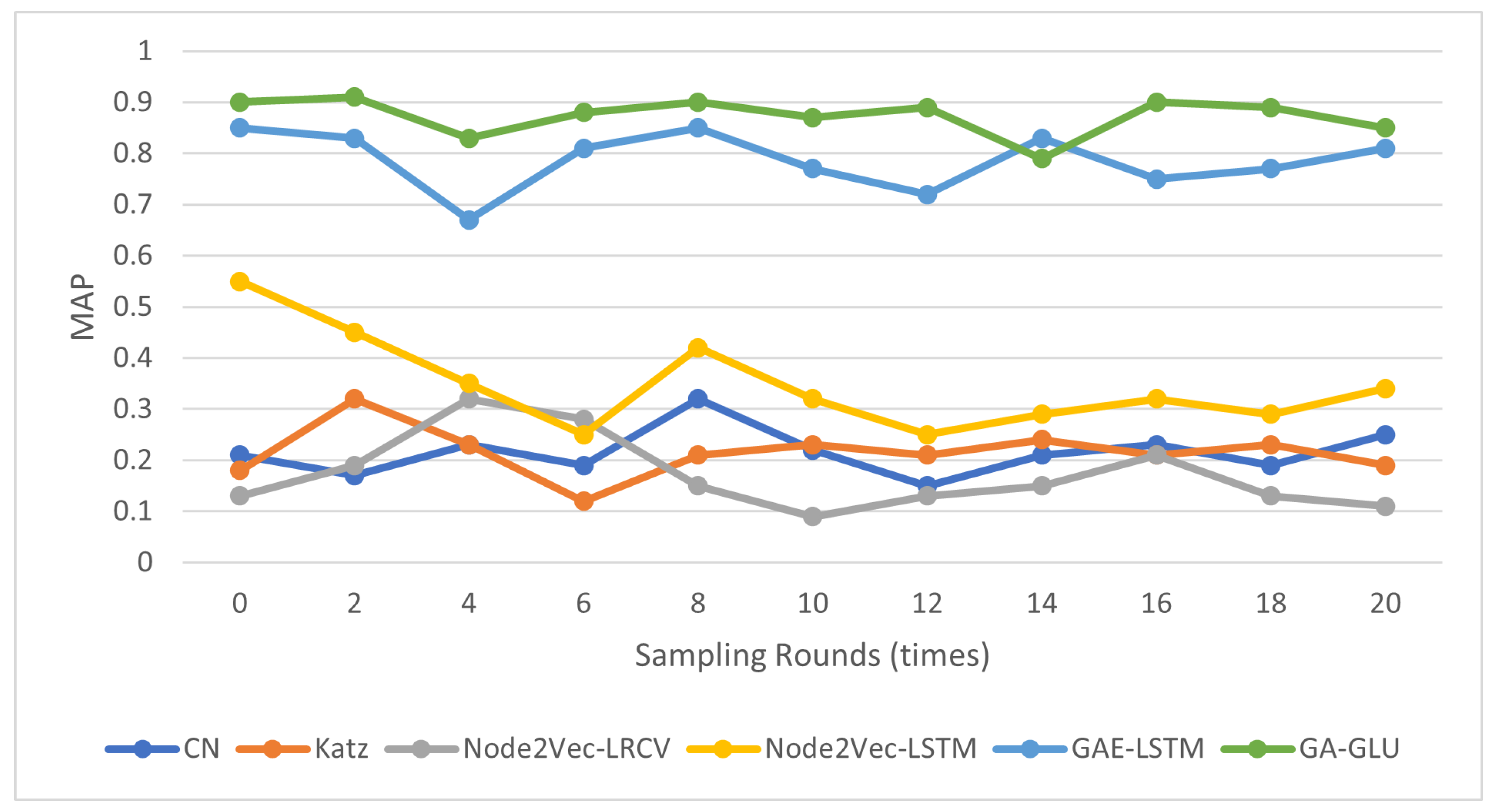
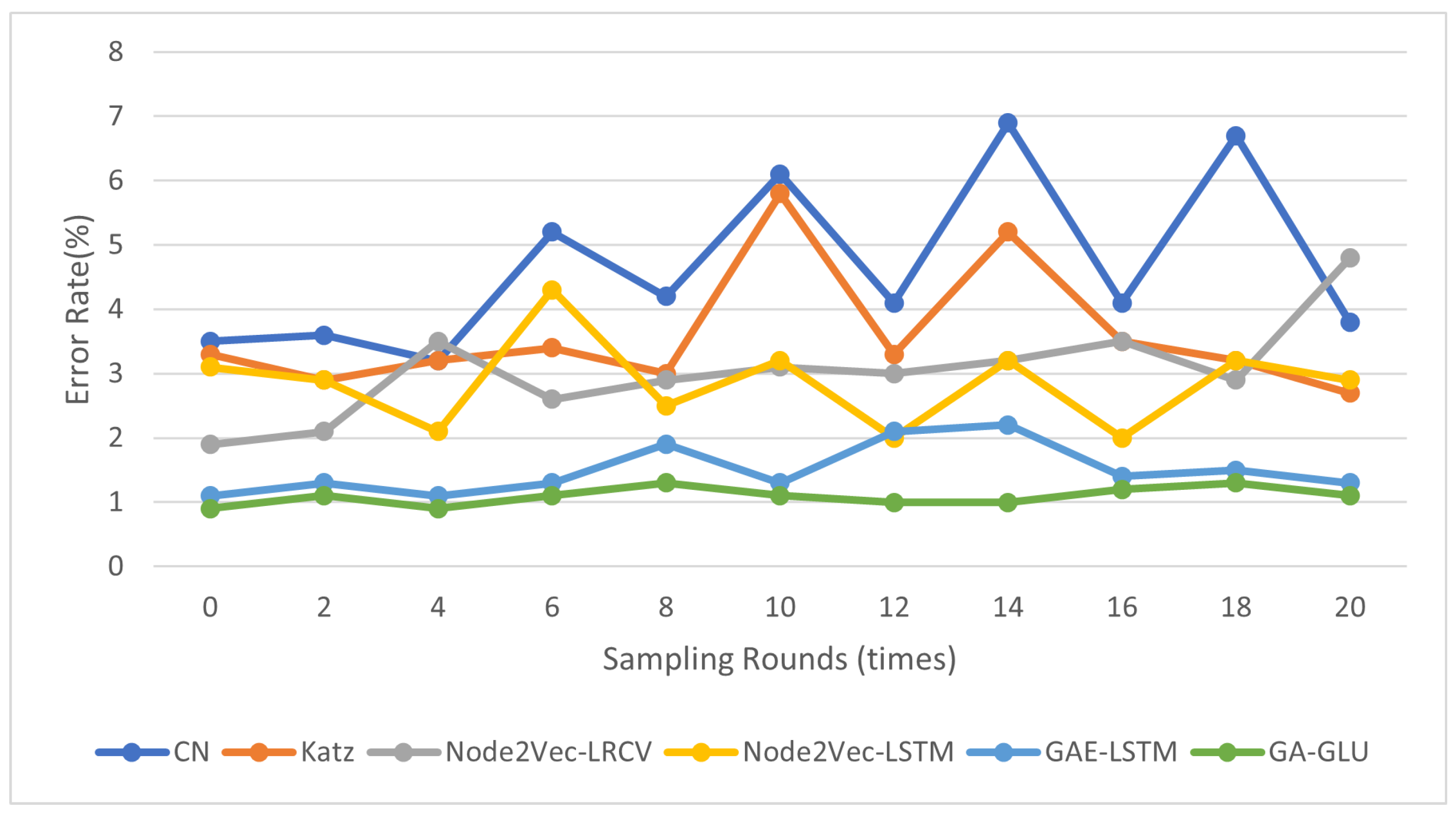
4.1. Link Prediction
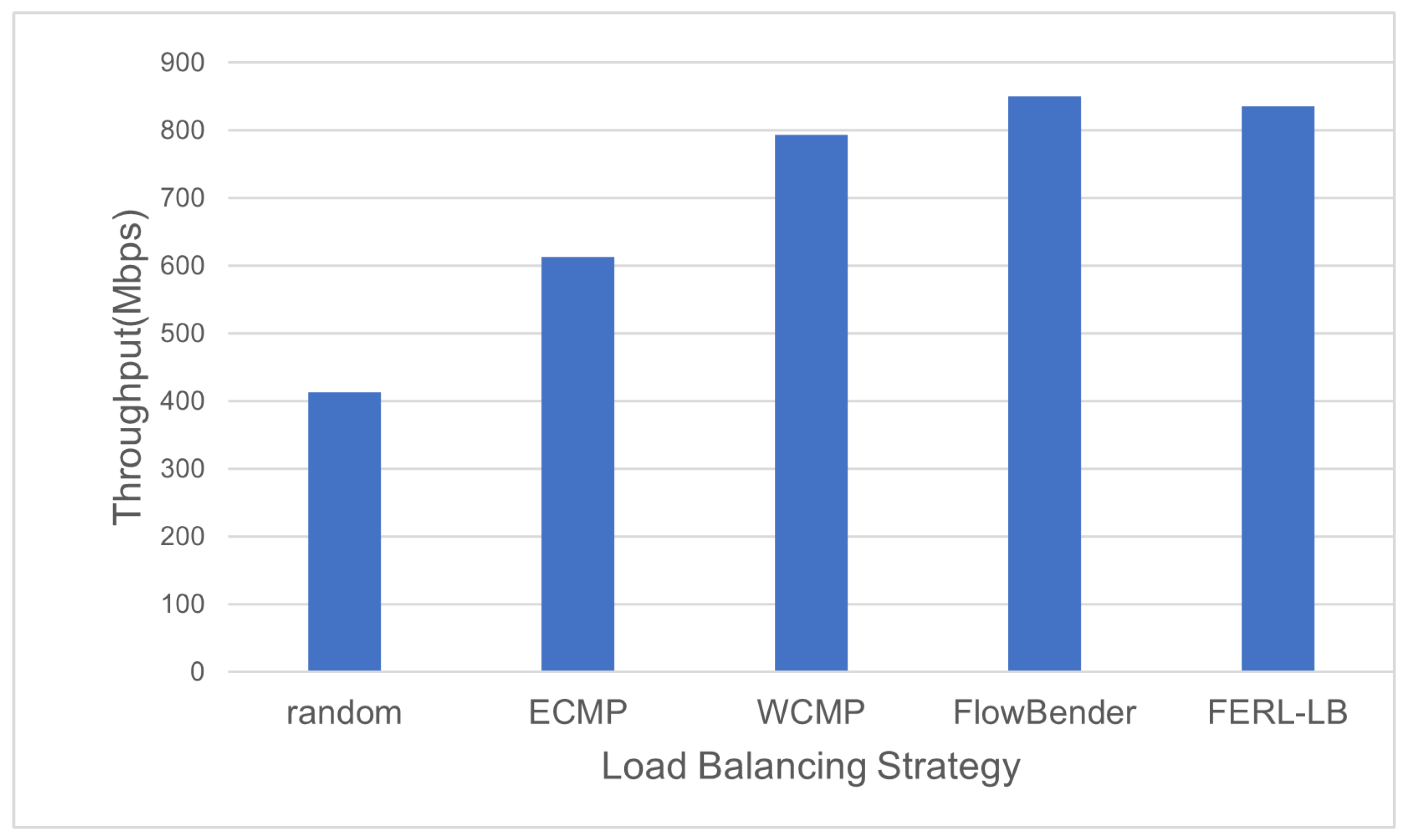
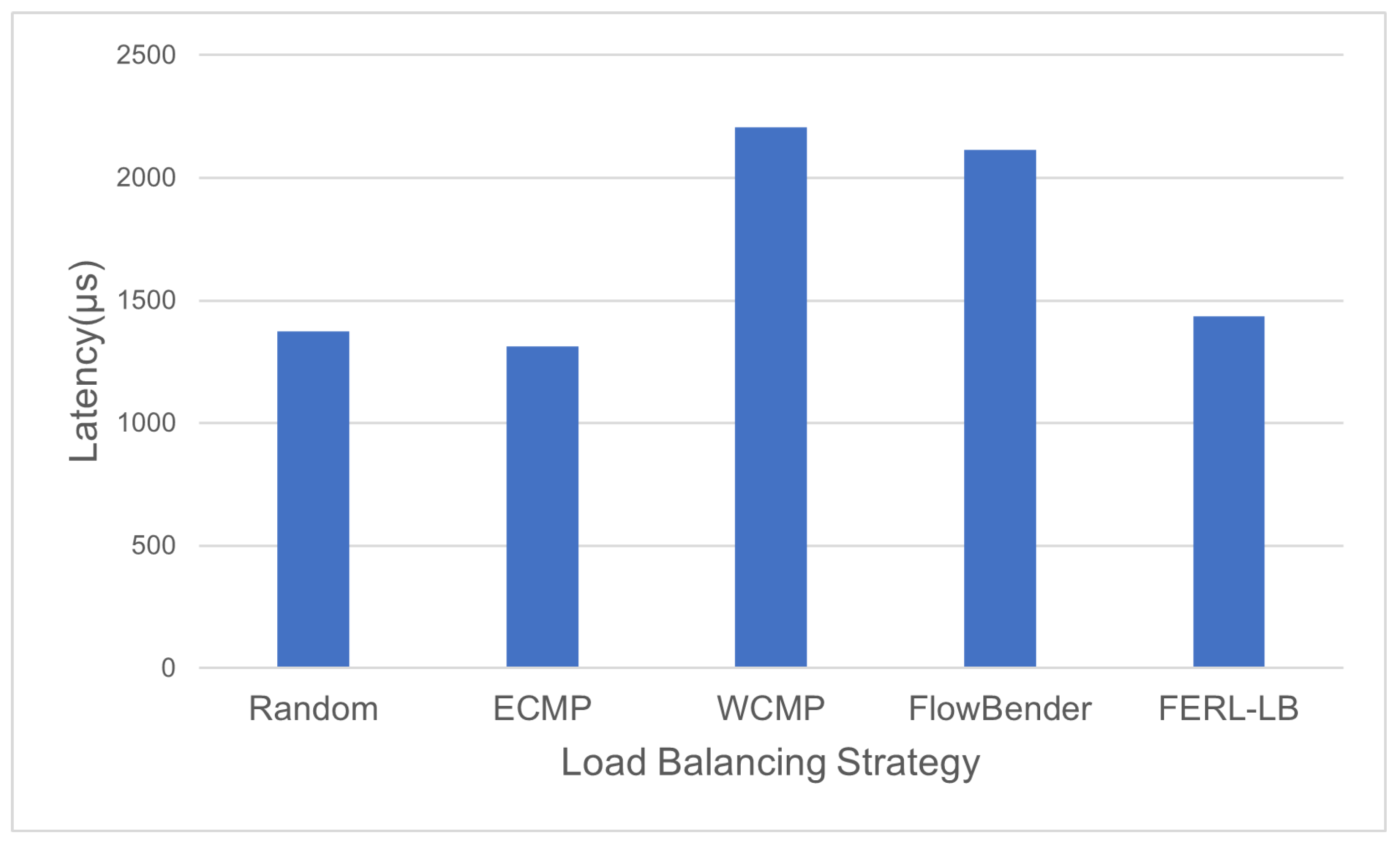
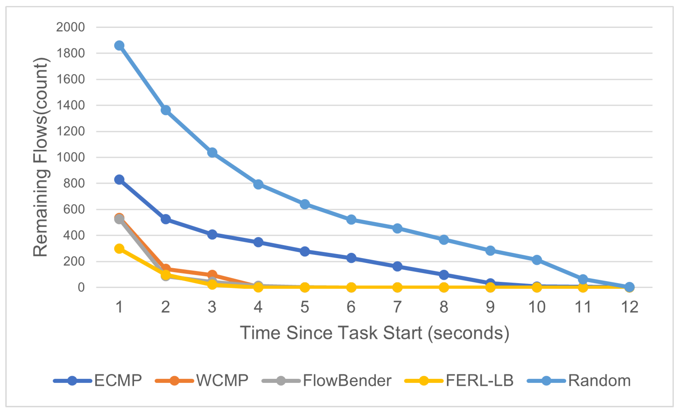
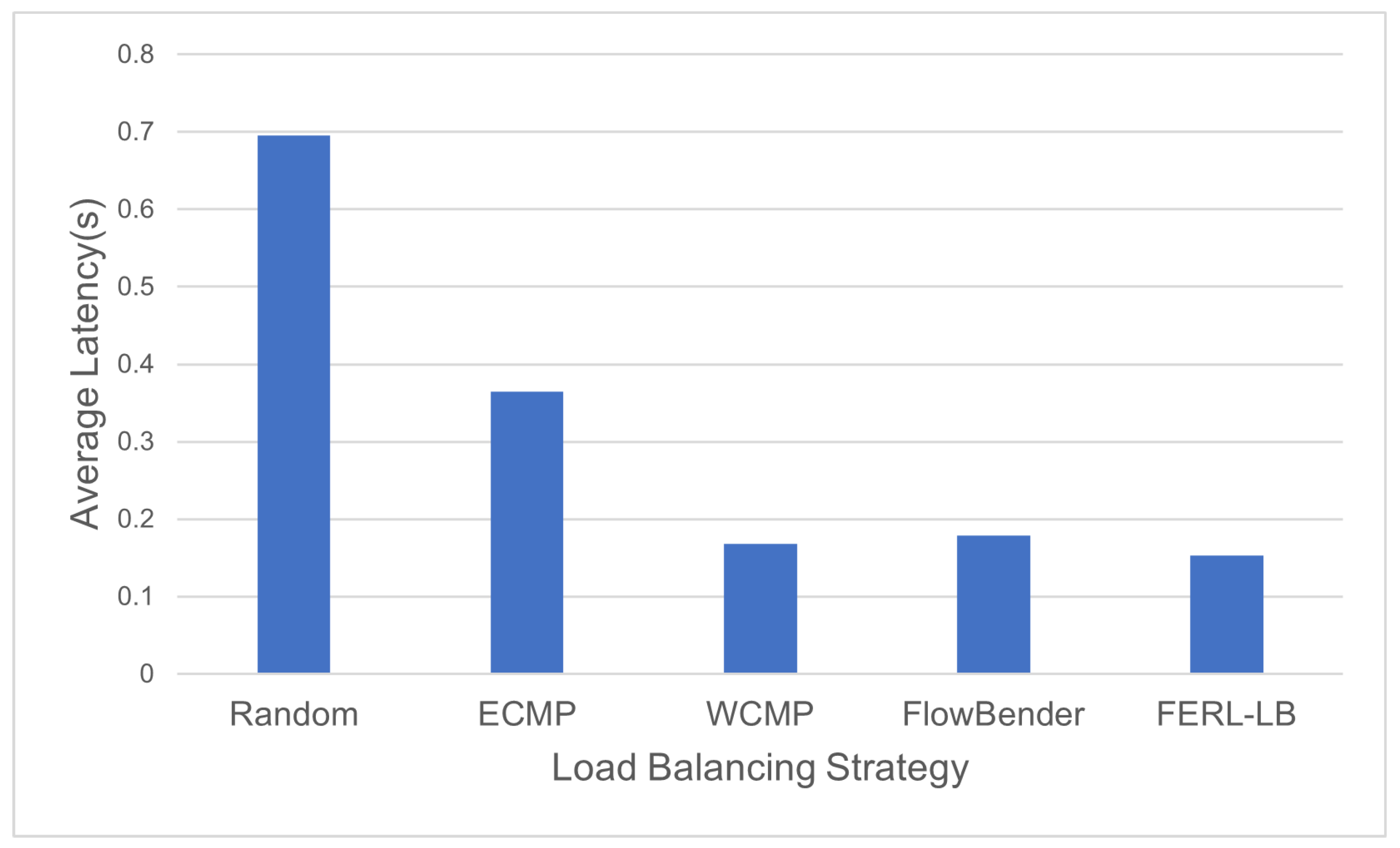
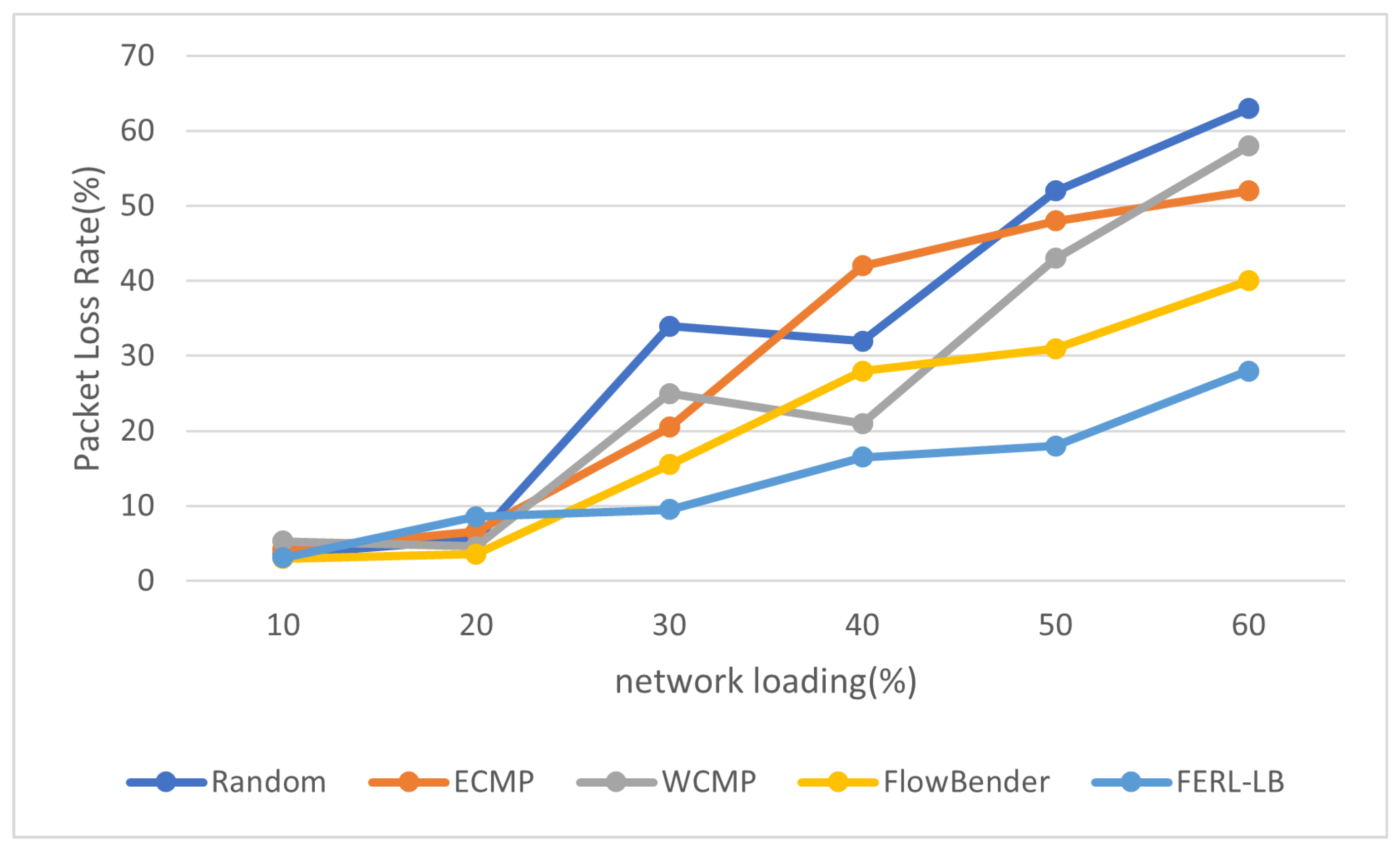
4.2. Load Balancing
5. Summary
Author Contributions
Funding
Data Availability Statement
Conflicts of Interest
References
- Gholami, A.; Baras, J.S. Collaborative cloud-edge-local computation offloading for multi-component applications. In Proceedings of the 2021 IEEE/ACM Symposium on Edge Computing (SEC), San Jose, CA, USA, 14–17 December 2021; pp. 361–365. [Google Scholar]
- Abbas, N.; Zhang, Y.; Taherkordi, A.; Skeie, T. Mobile edge computing: A survey. IEEE Internet Things J. 2017, 5, 450–465. [Google Scholar] [CrossRef]
- You, C.; Huang, K.; Chae, H.; Kim, B.H. Energy-efficient resource allocation for mobile-edge computation offloading. IEEE Trans. Wirel. Commun. 2016, 16, 1397–1411. [Google Scholar] [CrossRef]
- Li, X.; Chen, H. Recommendation as link prediction in bipartite graphs: A graph kernel-based machine learning approach. Decis. Support Syst. 2013, 54, 880–890. [Google Scholar] [CrossRef]
- Hayal, M.R.; Elsayed, E.E.; Kakati, D.; Singh, M.; Elfikky, A.; Boghdady, A.I.; Grover, A.; Mehta, S.; Mohsan, S.A.H.; Nurhidayat, I. Modeling and investigation on the performance enhancement of hovering UAV-based FSO relay optical wireless communication systems under pointing errors and atmospheric turbulence effects. Opt. Quantum Electron. 2023, 55, 625. [Google Scholar] [CrossRef]
- Ullah, S.; Mohammadani, K.H.; Khan, M.A.; Ren, Z.; Alkanhel, R.; Muthanna, A.; Tariq, U. Position-monitoring-based hybrid routing protocol for 3D UAV-based networks. Drones 2022, 6, 327. [Google Scholar] [CrossRef]
- Zhou, C.; Wu, W.; He, H.; Yang, P.; Lyu, F.; Cheng, N.; Shen, X. Delay-aware IoT task scheduling in space-air-ground integrated network. In Proceedings of the 2019 IEEE Global Communications Conference (GLOBECOM), Waikoloa, HI, USA, 9–13 December 2019; pp. 1–6. [Google Scholar]
- Kim, K.; Park, Y.M.; Hong, C.S. Machine learning based edge-assisted UAV computation offloading for data analyzing. In Proceedings of the 2020 International Conference on Information Networking (ICOIN), Barcelona, Spain, 7–10 January 2020; pp. 117–120. [Google Scholar]
- Jiang, F.; Wang, K.; Dong, L.; Pan, C.; Xu, W.; Yang, K. Deep-learning-based joint resource scheduling algorithms for hybrid MEC networks. IEEE Internet Things J. 2019, 7, 6252–6265. [Google Scholar] [CrossRef]
- Wang, L.; Wang, K.; Pan, C.; Xu, W.; Aslam, N.; Nallanathan, A. Deep reinforcement learning based dynamic trajectory control for UAV-assisted mobile edge computing. IEEE Trans. Mob. Comput. 2021, 21, 3536–3550. [Google Scholar] [CrossRef]
- Sanabria, P.; Montoya, S.; Neyem, A.; Toro Icarte, R.; Hirsch, M.; Mateos, C. Connection-Aware Heuristics for Scheduling and Distributing Jobs under Dynamic Dew Computing Environments. Appl. Sci. 2024, 14, 3206. [Google Scholar] [CrossRef]
- Bi, X.; Zhao, L. Two-Layer Edge Intelligence for Task Offloading and Computing Capacity Allocation with UAV Assistance in Vehicular Networks. Sensors 2024, 24, 1863. [Google Scholar] [CrossRef] [PubMed]
- Julian, K.; Lu, W. Application of machine learning to link prediction. arXiv 2016. [Google Scholar]
- Rahman, M.; Saha, T.K.; Hasan, M.A.; Xu, K.S.; Reddy, C.K. Dylink2vec: Effective feature representation for link prediction in dynamic networks. arXiv 2018, arXiv:1804.05755. [Google Scholar]
- Goyal, P.; Kamra, N.; He, X.; Liu, Y. Dyngem: Deep embedding method for dynamic graphs. arXiv 2018, arXiv:1805.11273. [Google Scholar]
- Li, T.; Zhang, J.; Philip, S.Y.; Zhang, Y.; Yan, Y. Deep dynamic network embedding for link prediction. IEEE Access 2018, 6, 29219–29230. [Google Scholar] [CrossRef]
- Chen, J.; Pareja, A.; Domeniconi, G.; Ma, T.; Suzumura, T.; Kaler, T.; Schardl, T.B.; Leiserson, C.E. Evolving Graph Convolutional Networks for Dynamic Graphs. US Patent 11,537,852, 7 December 2022. [Google Scholar]
- Lei, K.; Qin, M.; Bai, B.; Zhang, G.; Yang, M. GCN-GAN: A non-linear temporal link prediction model for weighted dynamic networks. In Proceedings of the IEEE INFOCOM 2019-IEEE Conference on Computer Communications, Paris, France, 29 April–2 May 2019; pp. 388–396. [Google Scholar]
- Min, S.; Gao, Z.; Peng, J.; Wang, L.; Qin, K.; Fang, B. Stgsn—A spatial–temporal graph neural network framework for time-evolving social networks. Knowl. Based Syst. 2021, 214, 106746. [Google Scholar] [CrossRef]
- Zhang, H.; Guo, X.; Yan, J.; Liu, B.; Shuai, Q. SDN-based ECMP algorithm for data center networks. In Proceedings of the 2014 IEEE Computers, Communications and IT Applications Conference, Beijing, China, 20–22 October 2014; pp. 13–18. [Google Scholar]
- Al-Fares, M.; Radhakrishnan, S.; Raghavan, B.; Huang, N.; Vahdat, A. Hedera: Dynamic flow scheduling for data center networks. In Proceedings of the USENIX Symposium on Networked Systems Design and Implementation, San Jose, CA, USA, 7–11 June 2010; Volume 10, pp. 89–92. [Google Scholar]
- Mao, B.; Tang, F.; Fadlullah, Z.M.; Kato, N. An intelligent route computation approach based on real-time deep learning strategy for software defined communication systems. IEEE Trans. Emerg. Top. Comput. 2019, 9, 1554–1565. [Google Scholar] [CrossRef]
- Sun, P.; Lan, J.; Li, J.; Zhang, J.; Hu, Y.; Guo, Z. A scalable deep reinforcement learning approach for traffic engineering based on link control. IEEE Commun. Lett. 2020, 25, 171–175. [Google Scholar] [CrossRef]
- Ruelas, A.M.; Rothenberg, C.E. A load balancing method based on artificial neural networks for knowledge-defined data center networking. In Proceedings of the 10th Latin America Networking Conference, New York, NY, USA, 3–5 October 2018; pp. 106–109. [Google Scholar]
- Babayigit, B.; Ulu, B. Deep learning for load balancing of SDN-based data center networks. Int. J. Commun. Syst. 2021, 34, e4760. [Google Scholar] [CrossRef]
- Gulrajani, I.; Ahmed, F.; Arjovsky, M.; Dumoulin, V.; Courville, A.C. Improved training of Wasserstein GANs. Adv. Neural Inf. Process. Syst. 2017, 30, 5767–5777. [Google Scholar]
- Kabbani, A.; Vamanan, B.; Hasan, J.; Duchene, F. Flowbender: Flow-level adaptive routing for improved latency and throughput in datacenter networks. In Proceedings of the 10th ACM International on Conference on Emerging Networking Experiments and Technologies, Sydney, Australia, 2–5 December 2014; pp. 149–160. [Google Scholar]
- Sun, P.; Hu, Y.; Lan, J.; Tian, L.; Chen, M. TIDE: Time-relevant deep reinforcement learning for routing optimization. Future Gener. Comput. Syst. 2019, 99, 401–409. [Google Scholar] [CrossRef]

| Algorithm | Advantages | Disadvantages |
|---|---|---|
| DyLink2Vec [14] | Efficient at capturing dynamic network changes; reduces reconstruction errors using gradient descent | Does not fully capture nonlinear patterns in temporal networks; struggles with scalability in large networks |
| DGEM [15] | Maps dynamic graph data to nonlinear latent space; effectively handles dynamic graph evolution | High computational cost; requires fine-tuning for optimal performance |
| DDNE [16] | Leverages historical data with GRUs to predict future link changes; effectively models temporal dependencies | Struggles to adapt in highly dynamic environments; performance heavily relies on temporal data quality |
| EvolveGCN [17] | Combines GCNs and RNNs to capture spatial and temporal dependencies; improves accuracy for evolving graphs | High model complexity; difficult to interpret results |
| STGSN [19] | Models both spatial and temporal features; utilizes attention mechanisms for better interpretability | High computational overhead; sensitive to noise in the data |
| GA–GLU (Proposed) | Combines a GAE, GANs, and LSTM networks for more accurate link prediction in UAV networks; captures both spatial and temporal dynamics; improves performance in highly dynamic environments | Requires careful tuning of GAN and LSTM components; slightly higher computational cost compared to simpler models |
| Configuration Parameter | Value |
|---|---|
| Number of UAVs | 36 |
| Simulation Duration (s) | 1000 |
| Max Speed (m/s) | 15 |
| Communication Range (m) | 500 |
| Starting Altitude (m) | 100 |
| Control Algorithm | Distributed Control |
| Scanning Phase Duration (s) | 0–500 |
| Hovering Phase Duration (s) | 500–1000 |
| Data Collection Frequency (Hz) | 10 |
| Network Type | Mesh |
| Method | AUC | MAP | Error Rate |
|---|---|---|---|
| CN | 0.883659 | 0.107073 | 4.038485 |
| Katz | 0.897741 | 0.118954 | 3.811238 |
| Node2vec-LRCV | 0.915489 | 0.157554 | 3.157558 |
| Node2vec-LSTM | 0.901738 | 0.409950 | 3.462399 |
| GAE–LSTM | 0.984325 | 0.777592 | 1.324715 |
| GA–GLU | 0.946060 | 0.756796 | 1.015201 |
Disclaimer/Publisher’s Note: The statements, opinions and data contained in all publications are solely those of the individual author(s) and contributor(s) and not of MDPI and/or the editor(s). MDPI and/or the editor(s) disclaim responsibility for any injury to people or property resulting from any ideas, methods, instructions or products referred to in the content. |
© 2024 by the authors. Licensee MDPI, Basel, Switzerland. This article is an open access article distributed under the terms and conditions of the Creative Commons Attribution (CC BY) license (https://creativecommons.org/licenses/by/4.0/).
Share and Cite
Long, H.; Hu, F.; Kong, L. Enhanced Link Prediction and Traffic Load Balancing in Unmanned Aerial Vehicle-Based Cloud-Edge-Local Networks. Drones 2024, 8, 528. https://doi.org/10.3390/drones8100528
Long H, Hu F, Kong L. Enhanced Link Prediction and Traffic Load Balancing in Unmanned Aerial Vehicle-Based Cloud-Edge-Local Networks. Drones. 2024; 8(10):528. https://doi.org/10.3390/drones8100528
Chicago/Turabian StyleLong, Hao, Feng Hu, and Lingjun Kong. 2024. "Enhanced Link Prediction and Traffic Load Balancing in Unmanned Aerial Vehicle-Based Cloud-Edge-Local Networks" Drones 8, no. 10: 528. https://doi.org/10.3390/drones8100528