4.1. Motion Sensors
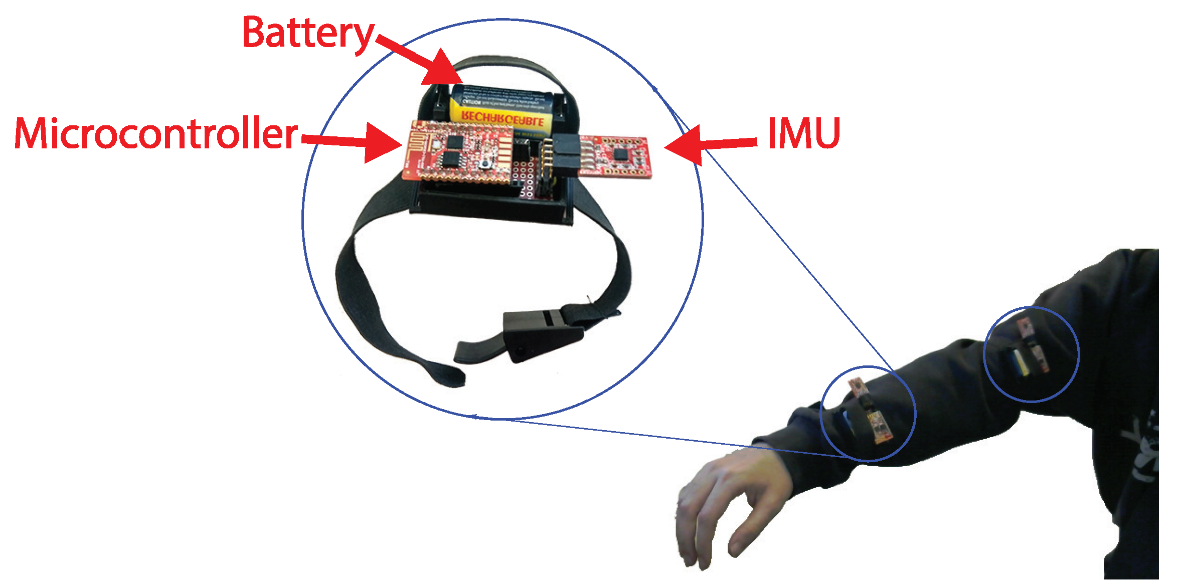
The implemented device, shown in
Figure 2, consists of inertial sensors that capture the node’s motion with respect to the inertial frame and a microcontroller with Wi-Fi capabilities. Specifically, the device consists of an IMU, a microcontroller and a removable and rechargeable small-size battery. The IMU that was used is a 9 DoF Micro-Electro-Mechanical System (MEMS) IMU. It is the single unit chip MPU-9150, produced by InvenSense Inc. The microcontroller that was used is a low-cost WiFi chip with full TCP/IP stack. It is the ESP8266 and it is produced by Espressif Systems [
48]. The purpose of this device is to retrieve and transmit the sensor data through WiFi to a base station. At the base station, the data is processed, stored and visualized. At last, the battery, which was used, is a removable RCR123A Lithium, high current, rechargeable battery that allows for a long-life and easy replacement.
Through an Inter Integrated Circuit (I
C) protocol [
49], the data received from the IMU sensors are used to estimate the orientation of the IMU chip. The ESP8266 micro-controller serves every device that requests data from the sensor node. The fact that HTTP protocol [
50] applies large headers, while it also lacks full duplex communication, makes this protocol not suitable for the designed application. Moreover, the time-restrictions and the requirement for transferring a great amount of data from the sensor to the base station, in a request-response messaging protocol, imposed the use of a more appropriate protocol. Thus, a websockets [
51] protocol was adopted. This protocol offers a persistent TCP/IP connection, while client and server can exchange packets, avoiding to burden the communication channel with a large volume of irrelevant data.
Each sensor node requires a calibration process before the first use. There are 3 sensors in the node and there is a different procedure for each sensor. For the magnetometer we should rotate the sensor multiple times at different directions. We store only the minimum and the maximum value on each axis. Having rotated for a while, we find the offset of each axis by taking the mean value of the maximum and minimum values for that axis. Then, we subtract this offset by the measurements. For the gyroscope, letting the device on a surface for a few seconds can produce the mean value of the sensor, which is supposed to be zero. Thus, we subtract this mean value from each measurement, in order to get the correct angular rotation of the device. The accelerometer calibration needs to lay the sensor with all its faces down. Hence, the gravity vector can be identified on each axis, and the values are saved on the microcontroller.
During the experimental sessions, a motion capturing sensor node is mounted on the outer side of the selected upper limb segment with the Y axis of the sensor being aligned with the longitudinal axis of the segment. The right placement of the sensor is ensured using a special designed fabric case, which is strapped in the circumference of the limb segment. Then, the sensor is switched on and the communication with the base station is established. The objectives are the acquisition, storing and concurrent visualization of the node’s IMU measurements during the subject’s exercise session.
Concurrently, a Shimmer3 sensor node [
26] has been aligned with the custom-made sensor, proposed in this work, and both were attached to the human’s upper limb segments. A custom-made piece with two sockets was used to successfully align these two sensors. The measurements form Shimmer3 sensor node were captured directly into Matlab
® using the Shimmer Matlab Instrument Driver. This driver is provided by the corresponding company and establishes the communication with the device via the Bluetooth protocol. Before the motion capturing session, the Shimmer3 units were calibrated using the Shimmer 9DOF Calibration Application, that is also derived by the same company. This application implements an automated process that calculates the calibration parameters for Shimmer’s integrated accelerometers, gyroscopes and magnetometers sensors. These calibration parameters are finally stored in the unit memory, so as the sensor measurements can be automatically corrected before they are sent to the paired device (e.g., a computer that functions as base station).
In the sequel, the collected sensors measurements, for both type of sensors, are processed and filtered as described in the previous Section. Then, the DoFs rotations
, for the upper limb model, are extracted by Equation (
12) for the shoulder, Equations (
13) and (
14) for the elbow and Equations (
15) and (
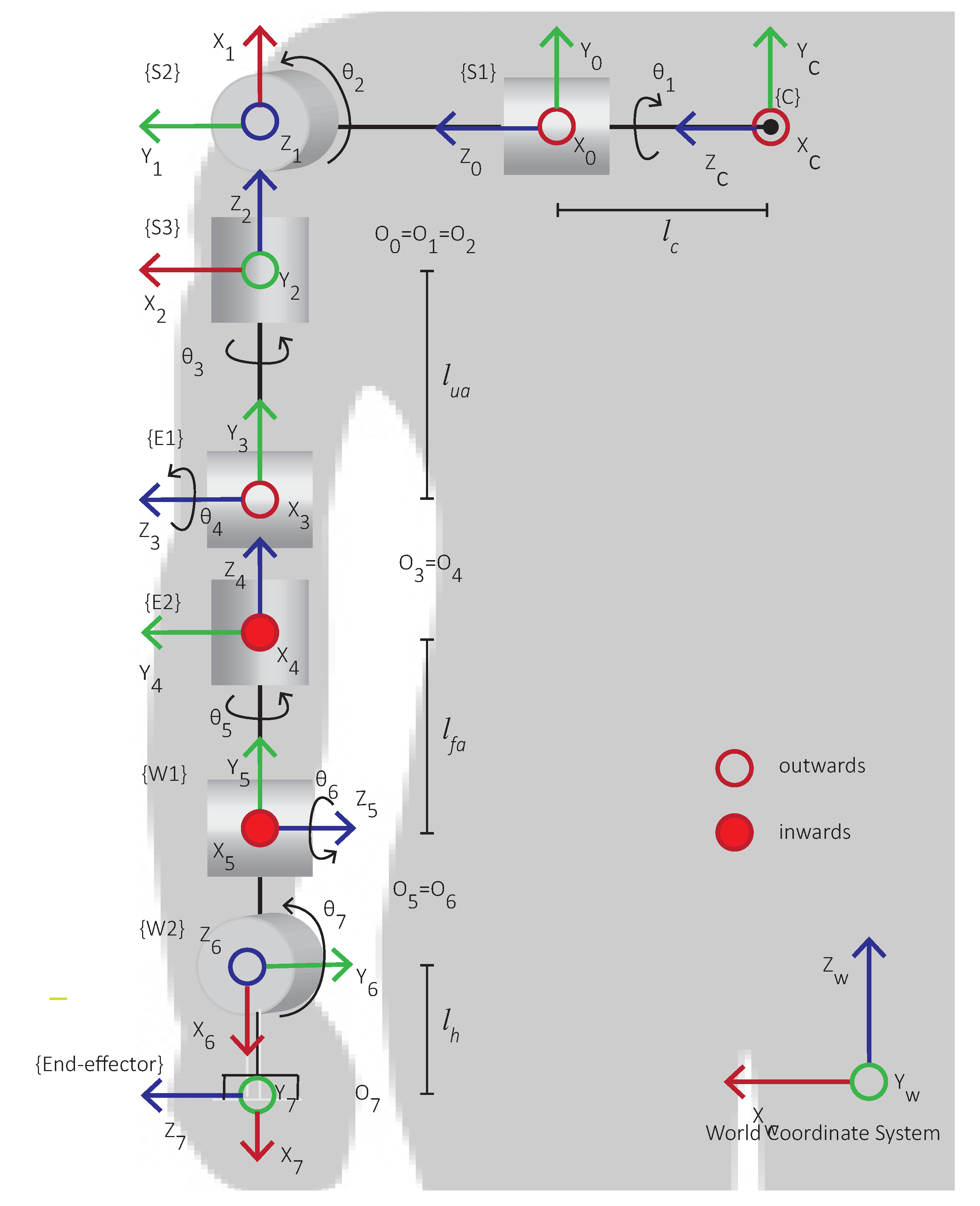
16) for the wrist joint, respectively. In the following Subsections, the 3D reconstructed upper limb joints trajectories are presented in common rehabilitation exercises, as the elbow’s flexion-extension, the shoulder’s abduction-adduction and the wrist’s flexion-extension exercise. In the processing stage, the sensor’s sampling period is selected as
msec, while the values of the model lengths are defined as
m,
m,
m and
m, which were estimated for the subject’s height of
m. Furthermore, the first two experimental cases do not account for any wrist rotation, since there was not any sensor node attached over the subject’s hand. Hence, the corresponding DoFs angles are assumed as
.
4.2. Elbow Joint Flexion-Extension Exercise
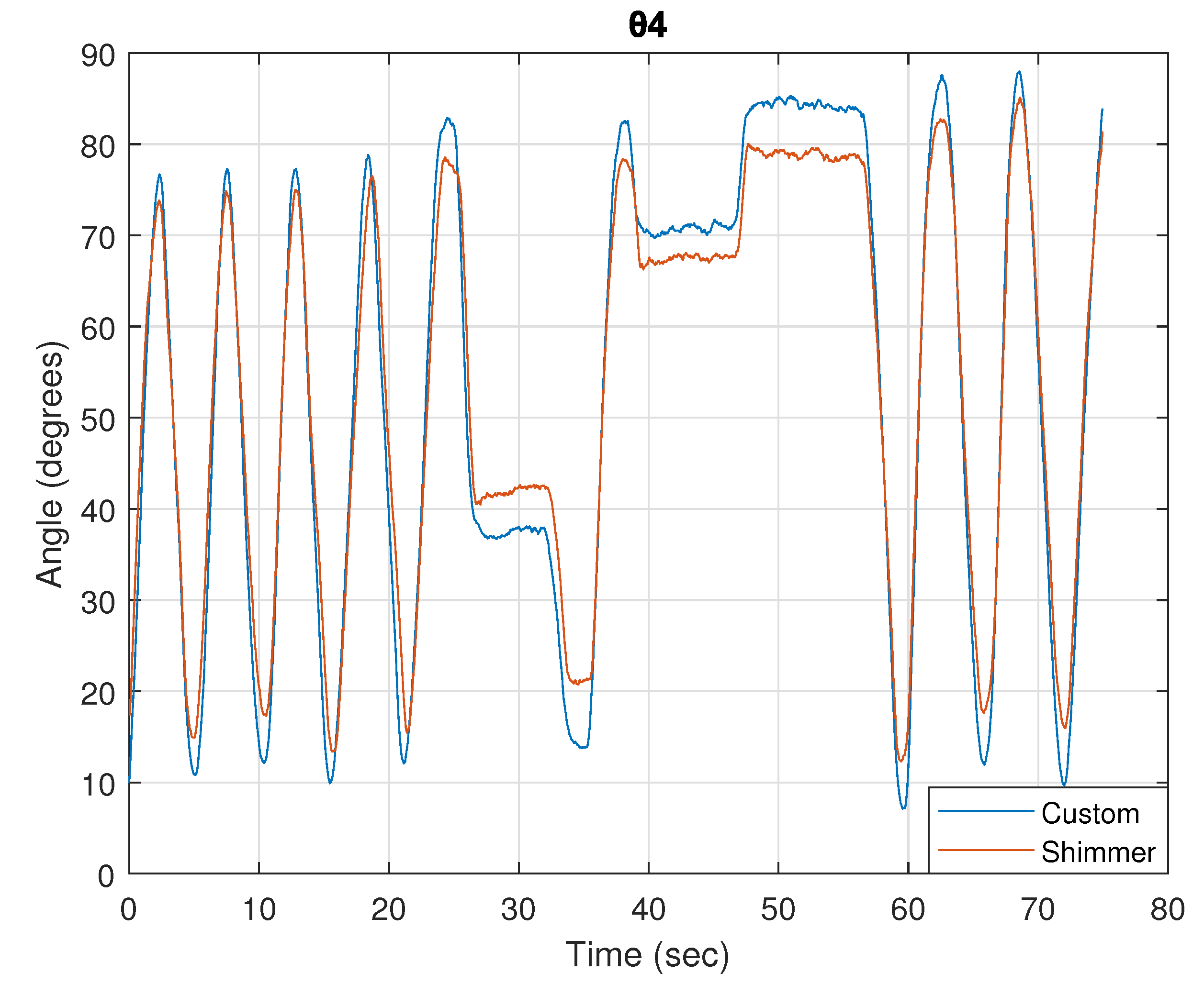
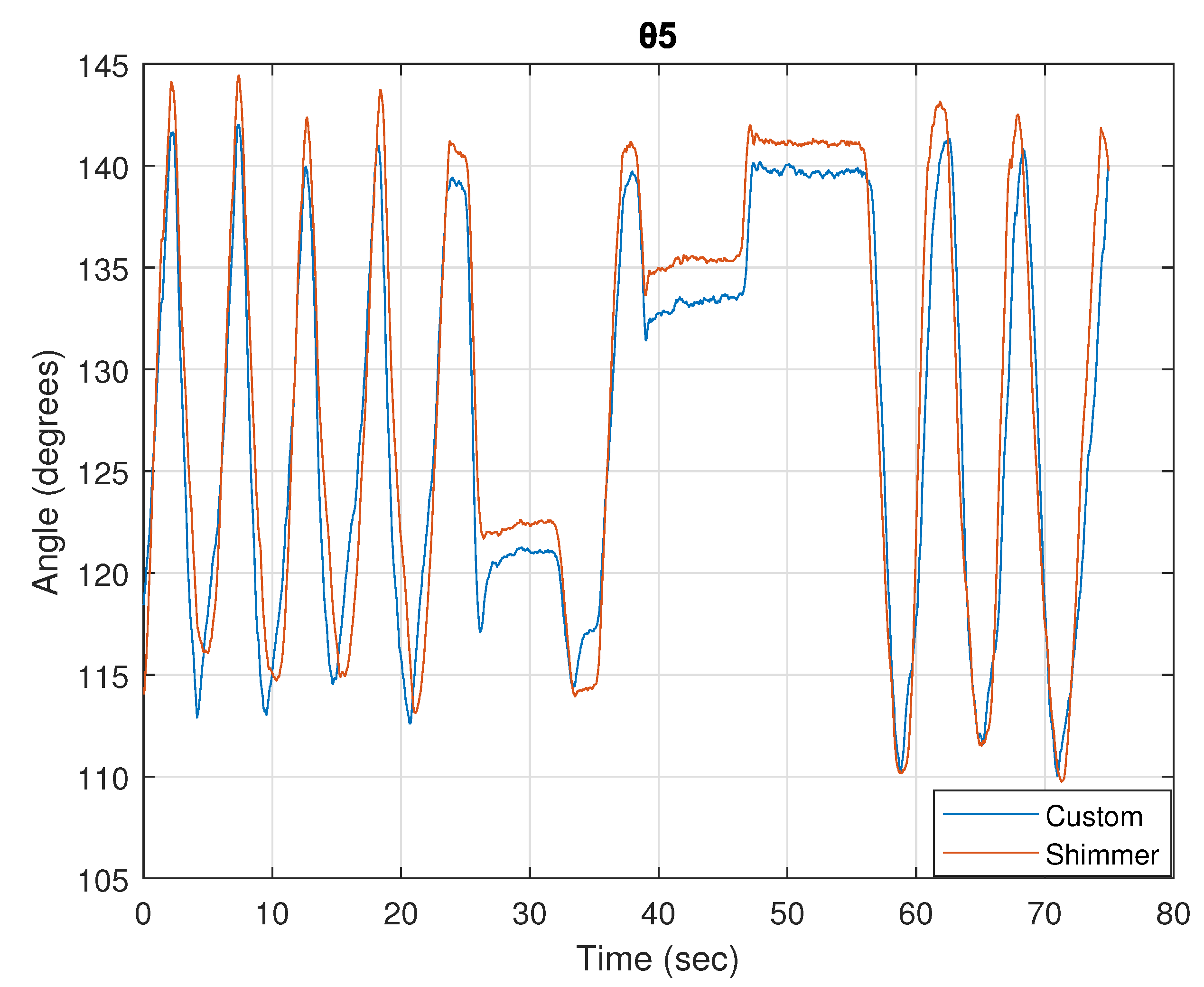
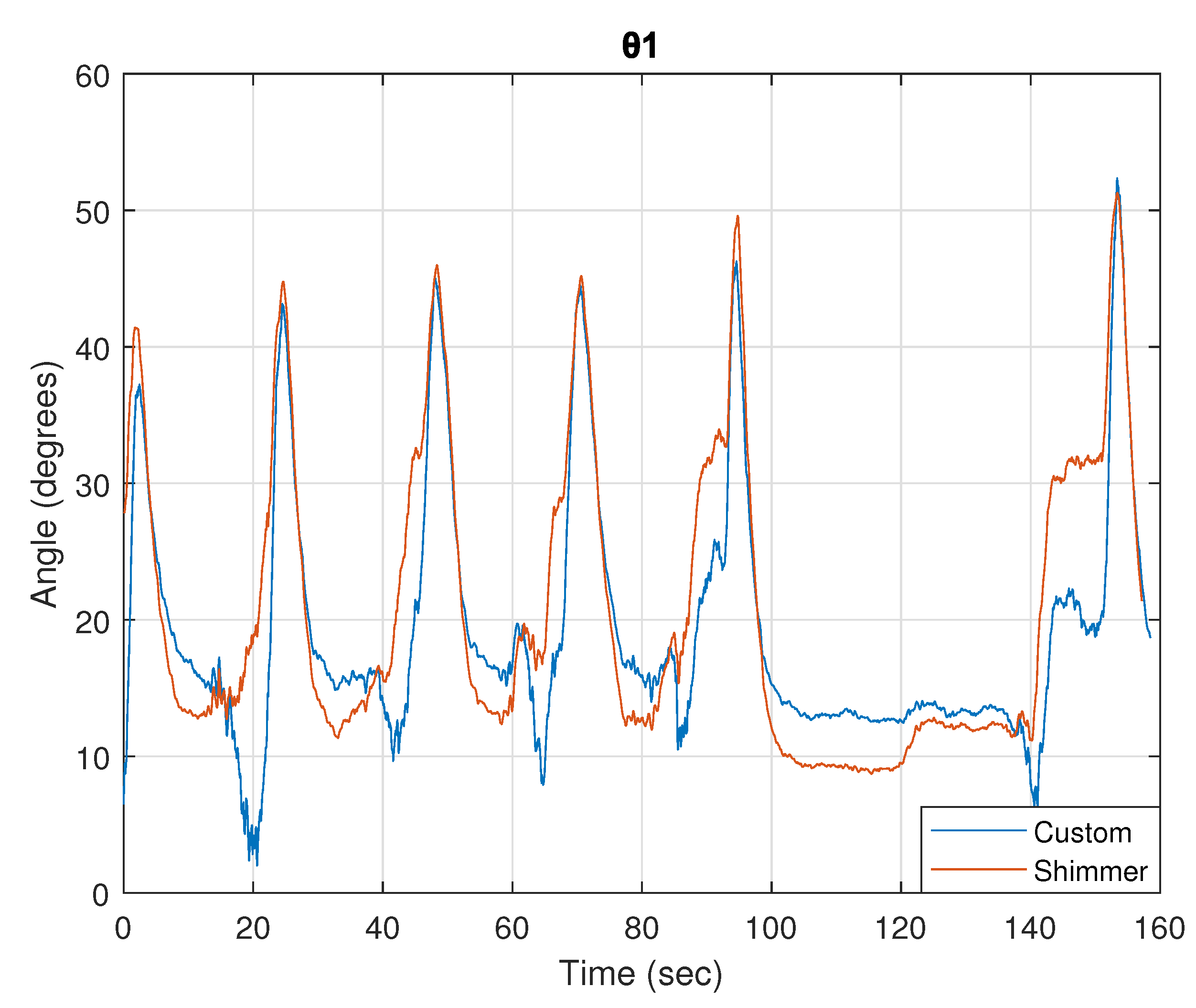
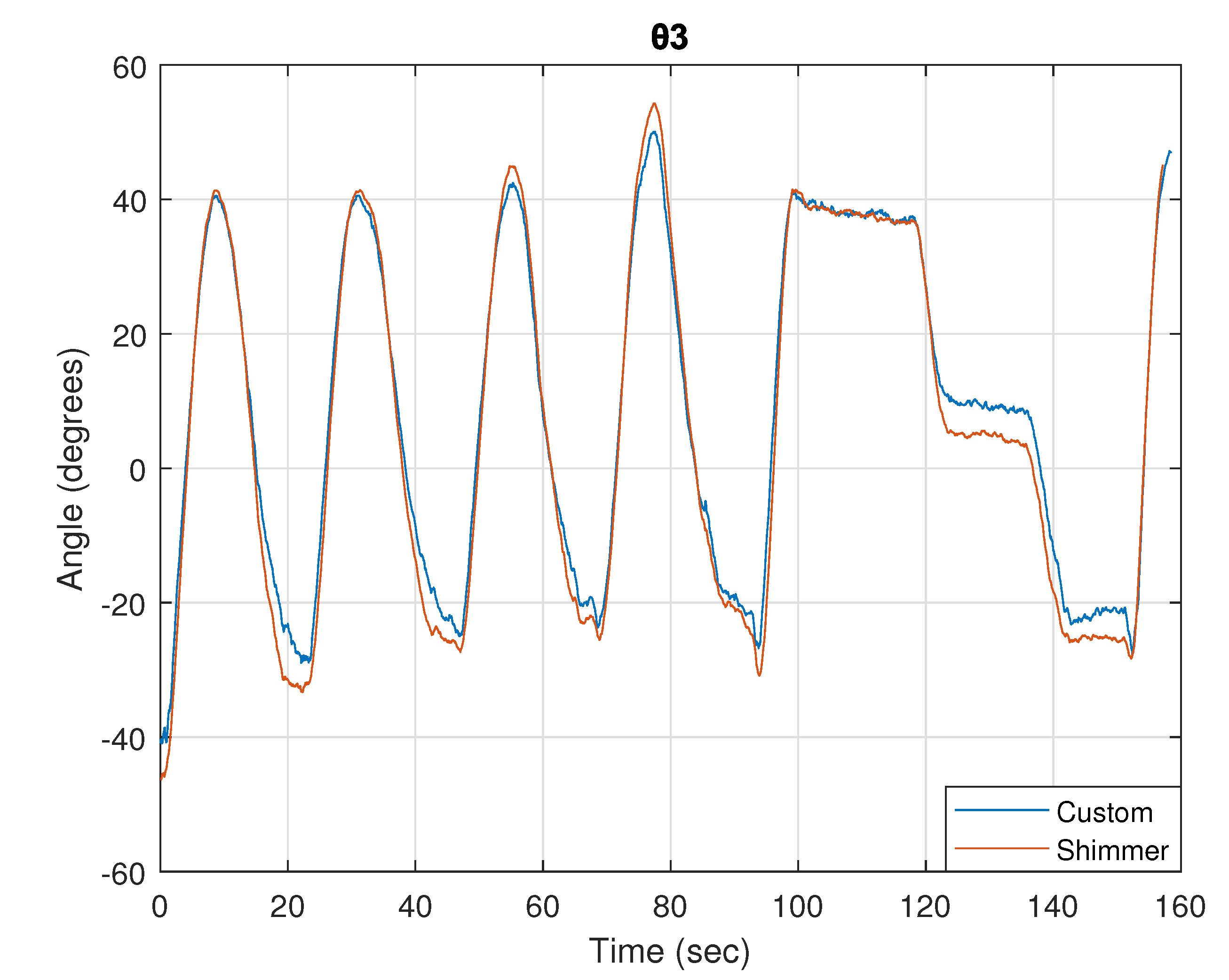
During this exercise session, the subject performs flexion and extension of the elbow. This exercise is repeated a few times and the sensor measurements of the node, which is attached to the subject’s forearm, are recorded and processed. This results to the estimation of the node’s orientation angles
,
and
. Using the node’s orientation angles, we can estimate the elbow DoF angles. Comparison between the proposed custom-made sensor node and the Shimmer3 sensor unit for the estimated angles
and
are shown in
Figure 3 and
Figure 4, respectively.
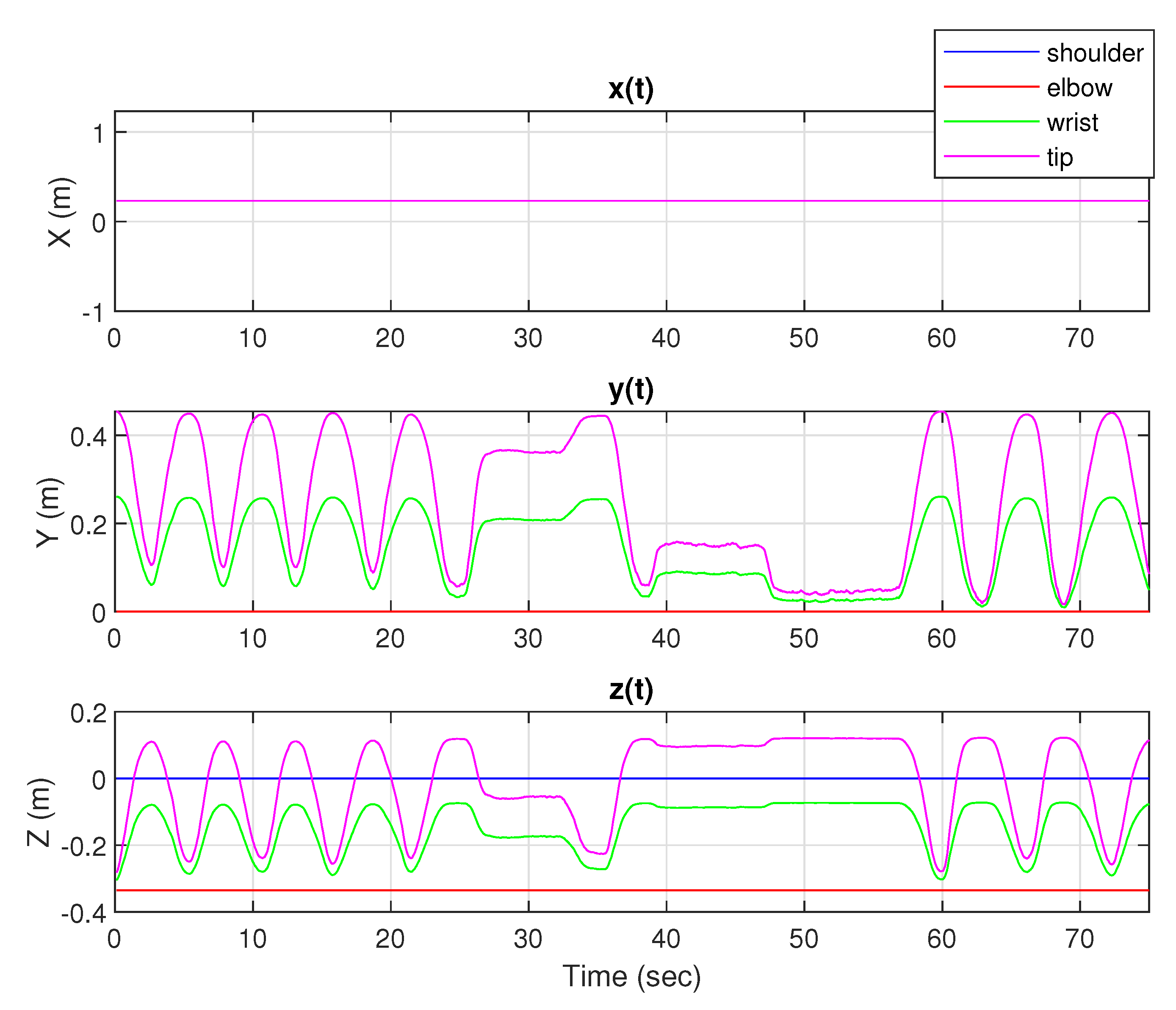
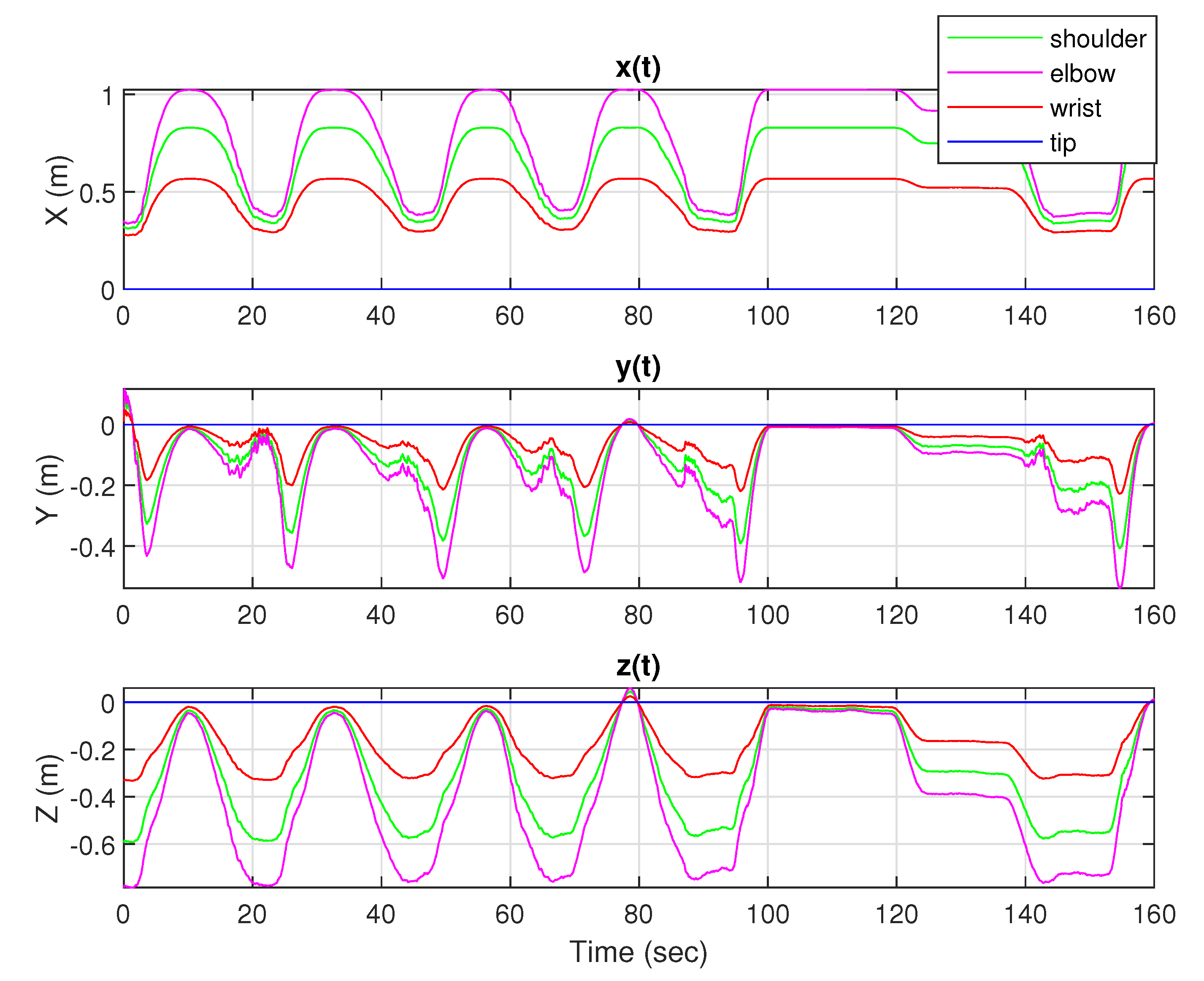
The trajectories of the shoulder, the elbow, the wrist joints and the tip of the hand in
x,
y, and
z axes are presented in
Figure 5. The distances between the segments joints, as shown in this figure, are in accordance with the corresponding fractions of human’s height. The motion takes place in the
plane and the value of
x component for each joint is constant and equal to the
, due to the dependence of the segments’ position only by the angle
. In this case, the position of the forearm is calculated by the transformation matrix
, which depends only on the variable
. The angle
affects only the orientation of the forearm and not its position. Furthermore, the hand is supposed to be aligned with the forearm, thus angles
and
of the wrist joint are zeroed.
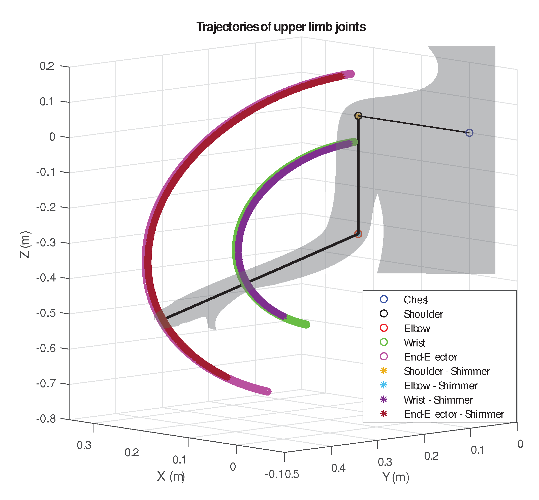
The resulted joints’ trajectories, as extracted by the upper limb model presented in
Section 2, for the calculated elbow DoF angles, are illustrated in
Figure 6. The trajectories, as extracted for the case of the custom-made sensor node, are noted with the ‘o’ symbol and represent the exercise that the patient has performed. The upper limb segments’ trajectories for the case of the Shimmer3 sensor unit’s measurements are also presented in the same figure. Deviations between the trajectories, especially in the upper and lower limit of the motion range, are identified in this figure. In the case of Shimmer3, the trajectories are more limited (noted with deep purple and deep red color). This is resulted by the elbow DoF angle
that ranges from
to
approximately, while the corresponding angle calculated by the measurements of the proposed sensor node ranges between
to
, as shown in
Figure 3.
The processing and filtering methodology, described in
Section 3.1, were followed for the IMU measurements of both sensor nodes. The nodes were calibrated before the capturing session. It was noticed that the differences in the elbow angles’ ranges, which were observed along a series of experiments, were related to the calibration accuracy of the sensors. Moreover, it was noticed that the forearm configuration during the exercise execution does not account for the gimbal lock problem. Finally, the points that are visualized in the trajectories’ 3D plots correspond to the total number of the exercise’s repetitions and not to only one.
The mean absolute error (MAE), the maximum error (MaxError) and root mean square error (RMSE) for the wrist and the tip of the hand (end-effector) trajectories, as were calculated between the proposed sensor node and the Shimmer one, are summarized in
Table 4.
Where
and the 3D trajectory points
for the custom-made sensor node and
for the Shimmer one are given as
, while
n denotes the total number of points of the trajectory. The estimated error metrics, which represent the difference among the trajectories extracted by these two sensor nodes, show a quite high level of accuracy.
4.3. Shoulder Joint Abduction-Adduction Exercise
Before the exercise session, we attach the wearable device to the subject’s upper arm. During this exercise session, the subject performs abduction and adduction of the shoulder joint for his right upper limb. The sensor’s on-board processor estimates the node’s orientation angles
,
and
. Then, it calculates the shoulder rotation angles
,
,
based on the procedure described above. The results are presented in
Figure 7,
Figure 8 and
Figure 9, accordingly, while the corresponding elbow angles
and
are fixed, during this exercise. As it is shown in the aforementioned figures, the shoulder’s joint angles, as extracted from both sensor nodes, are almost identical. Therefore, an accurate reconstruction of the upper limb movement can be achieved either using a shimmer sensor node or the proposed custom-made one.
The trajectories of the shoulder, the elbow, the wrist and the tip of the hand in
x,
y, and
z axes are presented in
Figure 10. Deviations in the
y axis occur, while the subject’s motion took place in the
(sagittal) plane. This was caused because of the not ideal mounting of the node on the subject’s upper arm and, thus, a sensor-to-body frame transformation should be defined.
An issue that might occur during this motion is the gimbal lock problem. This results from the use of the Euler orientation angles , and to find, after processing, the position and orientation of the corresponding segment. Actually, the shoulder joint can perform three rotations. When the angle rotation comes up to the furthest point, the shoulder joint axes and of the first and third shoulder’s DoF, accordingly, are collinear. This is a singular configuration and only the sum or the difference can be determined. One solution is to choose the one angle arbitrarily and then determine the other using trigonometric equations. Nevertheless, the range of motion in the present exercise is not affected by the gimbal lock issue.
The 3D reconstructed trajectories of each upper limb joint are presented in
Figure 11, noted with ’o’ symbol, for the case of the custom-made sensor node. A few consecutive repetitions of abduction-adduction exercise are performed, which explains the deviations of the visualized points. The extracted upper limb segments’ trajectories for the case of the Shimmer3 unit are also presented in the same figure. As in the comparison of the previous exercise (elbow flexion-extension), the trajectories of the upper limb segments, which are extracted from the Shimmer3 sensor’s measurements (noted with light blue, deep purple and deep red color), are more limited than the corresponding ones resulted from the custom-made motion capture sensor node. This results from the minor differences in the calculated shoulder DoFs’ ranges between the two sensors nodes. Once again, in this experiment, it was observed that the shoulder angles’ ranges were related to the accuracy of the calibration parameters for each sensor.
The mean absolute error (MAE), the maximum error (MaxError) and root mean square error (RMSE) for the elbow, wrist and tip of the hand (end-effector) trajectories, between the two sensor nodes, as extracted using Equations (
17), are summarized in
Table 5.
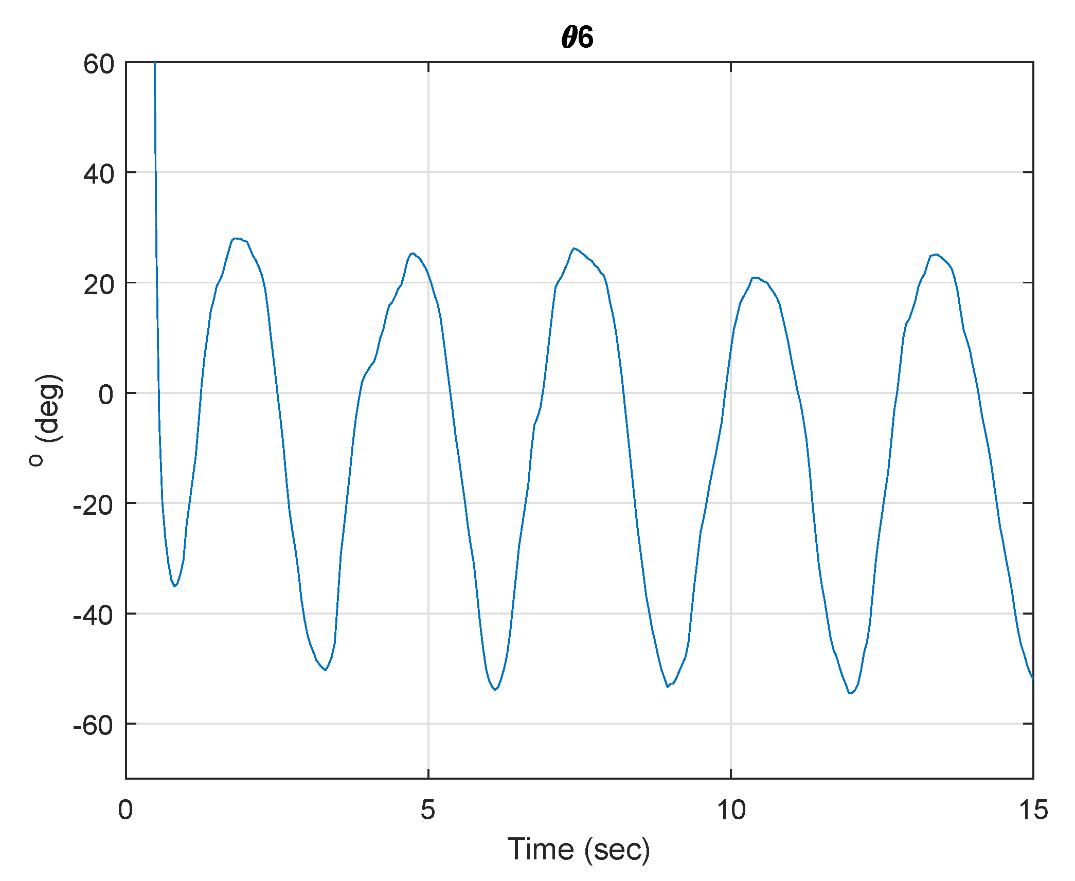
4.4. Wrist Joint Flexion-Extension Exercise
In this case, the subject performs a few repetitions of wrist joint flexion-extension exercise of his right upper limb. The extracted sensor orientation angles
,
and
contribute to the wrist DoFs angles estimation. During this exercise the subject’s elbow is steadily flexed at
being perpendicular to the coronal plane, and the hand is repeatably flexed with the palm towards the chest at almost
and extended until almost
, as shown in
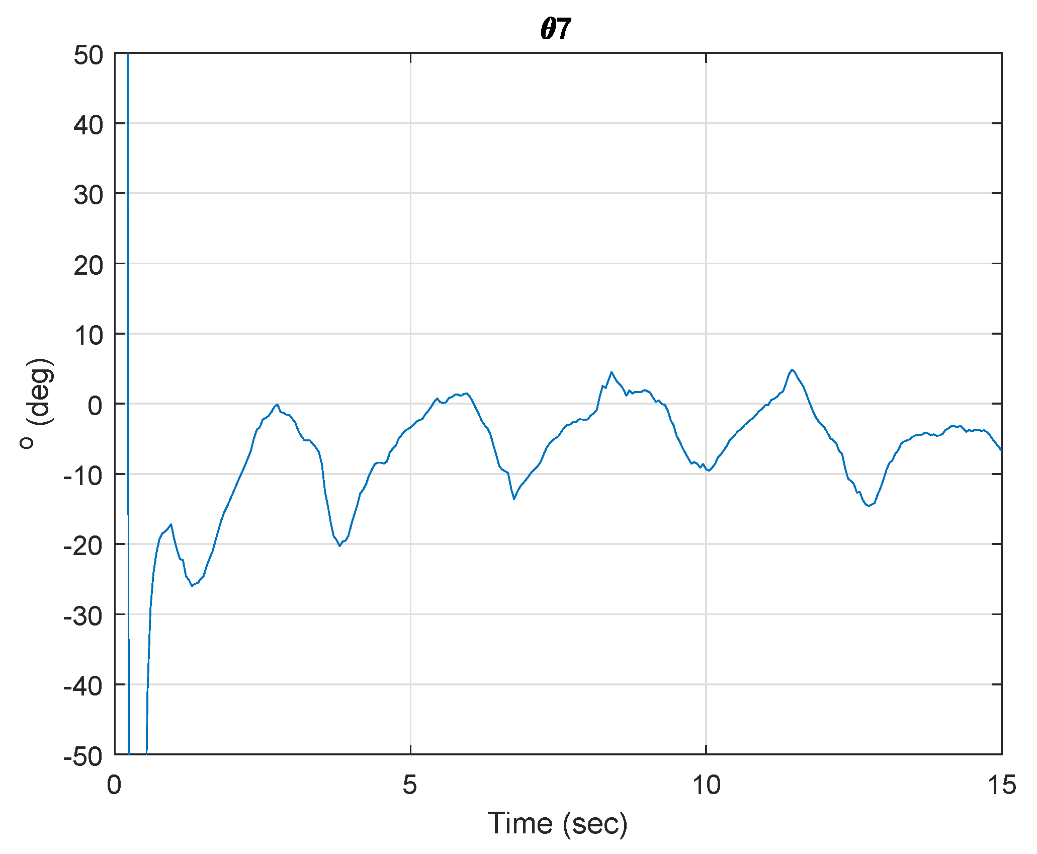
Figure 12. In
Figure 13, a deviation around a mean value is presented that corresponds to the second DoF of the wrist, this of radial-ulnar deviation. Actually, a small deviation is present during the subject’s wrist motion, thus the deviation in this graph is reasonable.
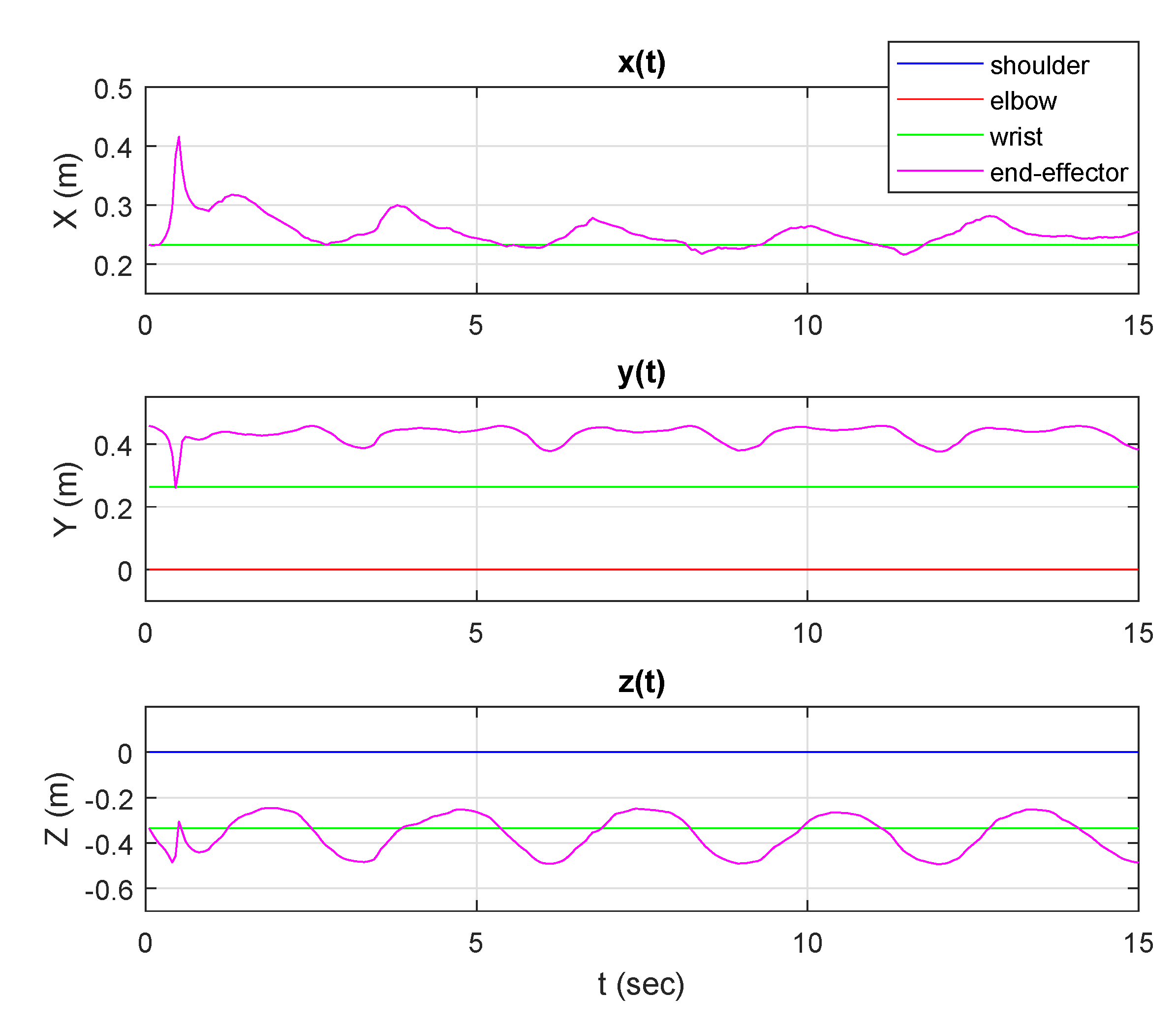
The concluded joints’ trajectories, as extracted by the upper limb model for the wrist DoF angles
and
is illustrated in
Figure 14. It represents the exercise that the subject has performed, along with this small deviation. The corresponding trajectories of the shoulder, the elbow, the wrist and the tip of the hand in
x,
y, and
z axes are presented in
Figure 15.
In this case, a comparison among the custom-made and the Shimmer3 sensor node was not realized, because it was not possible to attach the array of the aligned sensors on the subject’s hand, due to the hardware dimensions.
Such graphs of upper limb trajectories and joint DoFs angles during exercise sessions are useful for a subject’s upper limb status evaluation by the physical therapists. Especially, the analysis over the range of motion for each joint angle or even the estimation of the speed during the execution of an exercise indicate the status and progress of a patient with upper limb movement disorders. Hence, the therapists could tune the sequel rehabilitation sessions accordingly.


