3.1. Experiment Description
The research object in this study is the TV3-117 aircraft engine, which belongs to the helicopter TE class. The sensor in the sensory system consists of 14 T-101 thermocouples, which record the gas temperature before the compressor turbine
value on board the helicopter (1 value per second) (
Table 1) [
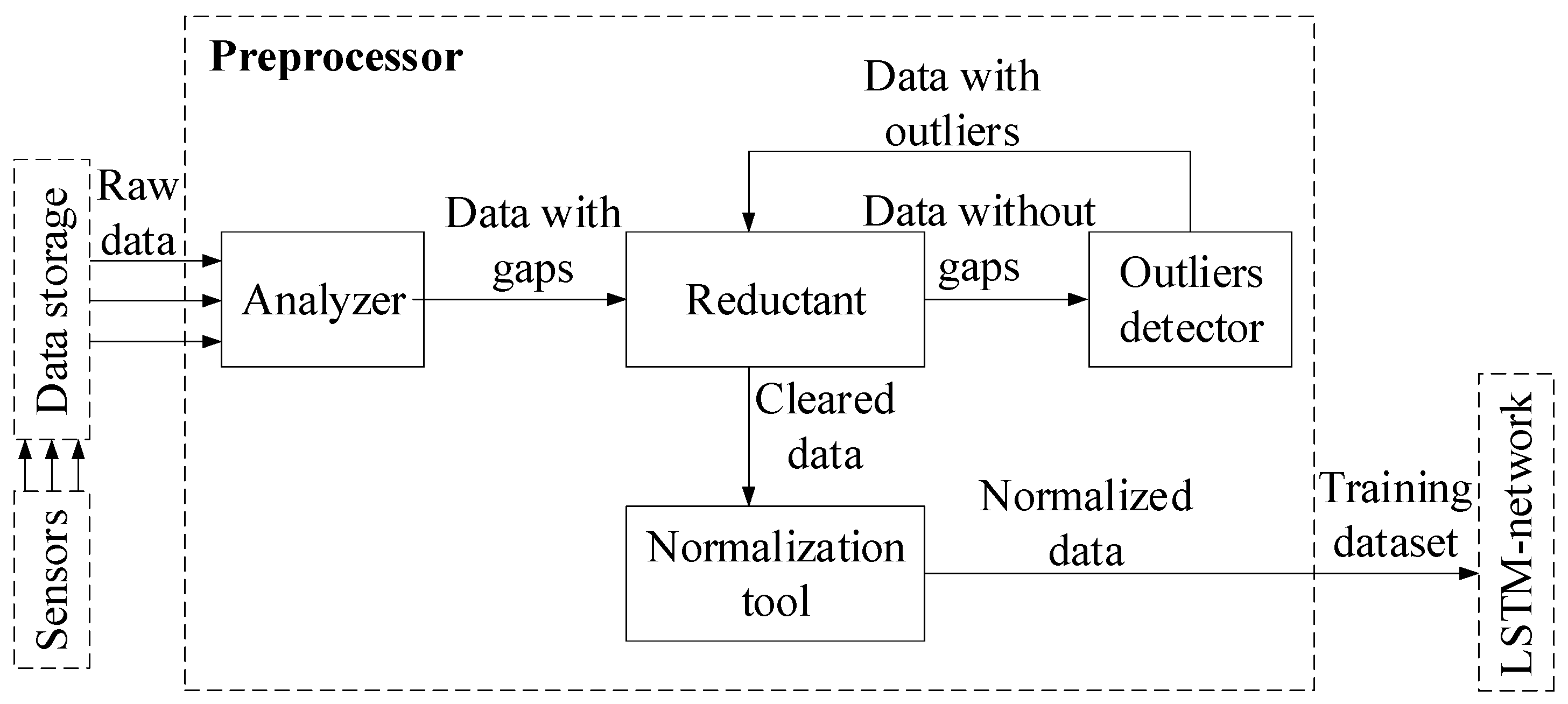
41]. The preprocessor is implemented using Python libraries as follows. The analyzer uses the standard libraries “openpyxl” and “pandas”. The outlier detector is based on algorithms from the “adtk” (Anomaly Detection Toolkit) library [
42]. The
SARIMAX model, used by the restorer, is implemented in the standard “statsmodels” library. The normalizer is implemented using the standard “sklearn” library. The predictor is implemented based on the Keras library [
43] and the TensorFlow framework [
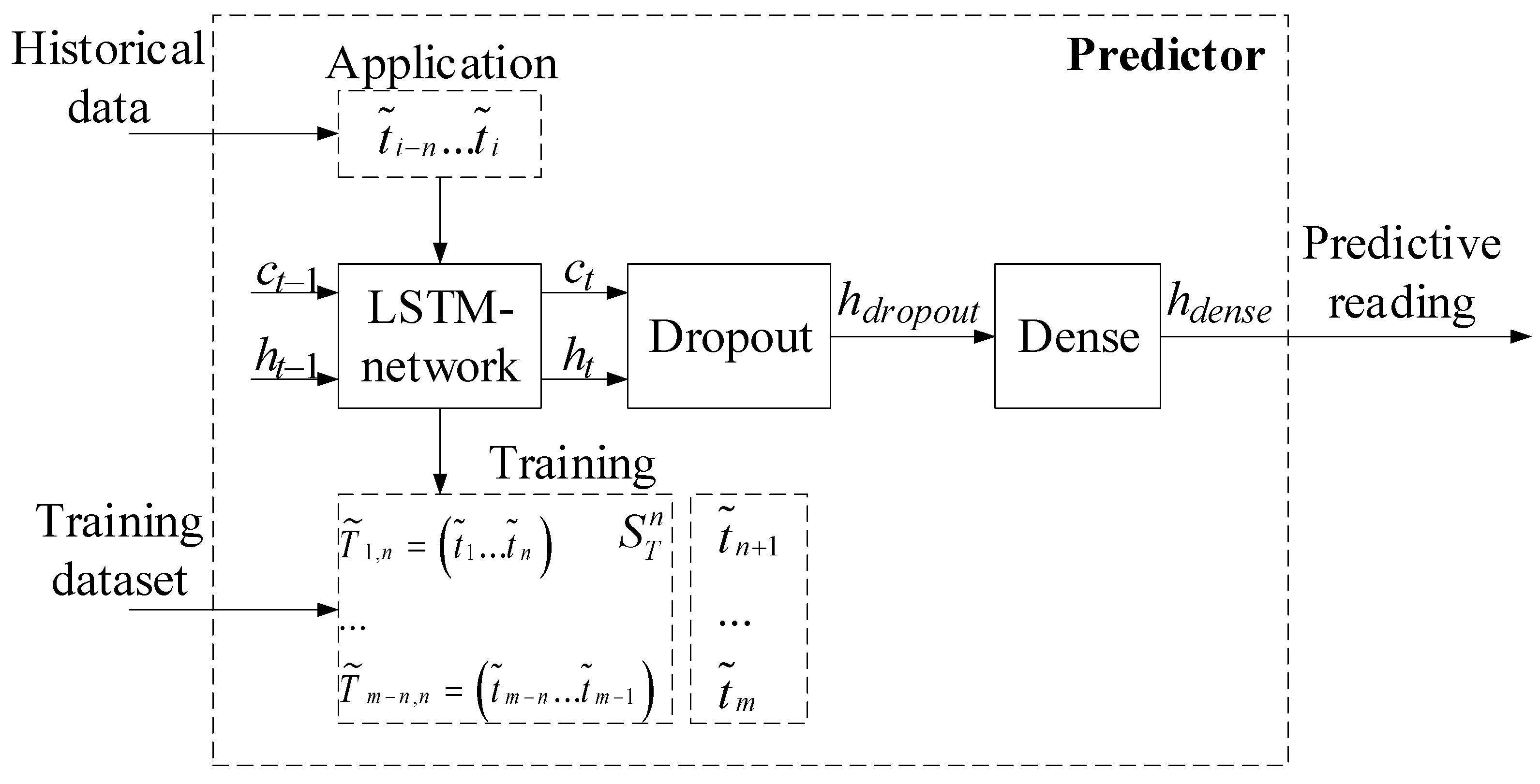
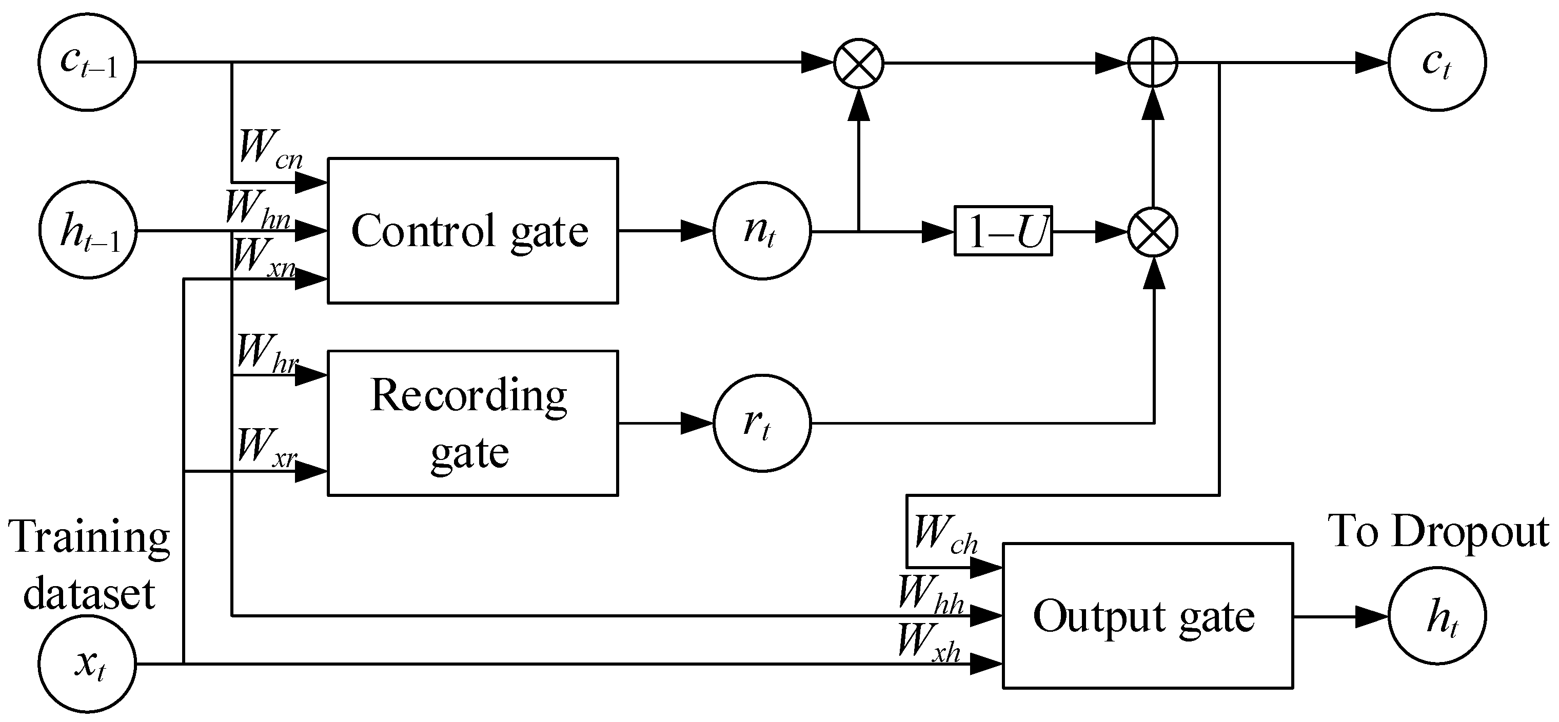
44]. For training the recurrent neural network, subsequences of length
n = 256 were used, corresponding to 256 s of sensor operation. The RNN hidden state was taken as a column vector of length ∣
h∣ = 32. The following commonly accepted parameters were used for network training: the loss function was
MSE (Mean Square Error), the optimizer was Adam, and the epochs and batch size number were 20 and 32, respectively. The anomaly detector was implemented using the “MatrixProfile library” for the Python 3.12.4 programming language [
45].
The training dataset (
Table 1) homogeneity evaluation using Fisher–Pearson [
46] and Fisher–Snedecor [
47] criteria is detailed in [
41]. According to these criteria, the training dataset of gas temperature readings before the compressor turbine for the TV3-117 aircraft engine is homogeneous, as the calculated values for the Fisher–Pearson and Fisher–Snedecor criteria are below their critical values, i.e.,
и
. To assess the representativeness of the training dataset, ref. [
41] employed cluster analysis (k-means [
48,
49]). Using random sampling, the training and test datasets were divided in a 2:1 ratio (67% and 33%, corresponding to 172 and 84 elements, respectively). The cluster analysis results for the training dataset (
Table 1) identified eight classes (classes I …VIII), indicating the presence of eight groups and demonstrating the similarity between the training and test datasets (
Figure 5).
These results enabled the optimal sample sizes for the determination of gas temperature before the compressor turbine for the TV3-117 aircraft engine: the training dataset comprises256 elements (100%), the validation dataset comprises 172 elements (67% of the training dataset), and the test dataset comprises84 elements (33% of the training dataset).
After the processing of data by the preprocessor, the first 172 values (67%) from the sensor (control dataset) were used in two roles: as a dataset for tuning the SARIMAX model parameters used by the reconstructor and as the training dataset for the recurrent neural network in the predictor subsystem. The remaining 84 values (33%) from the sensor (test dataset) were used for the data cleaning module operation simulated under normal conditions.
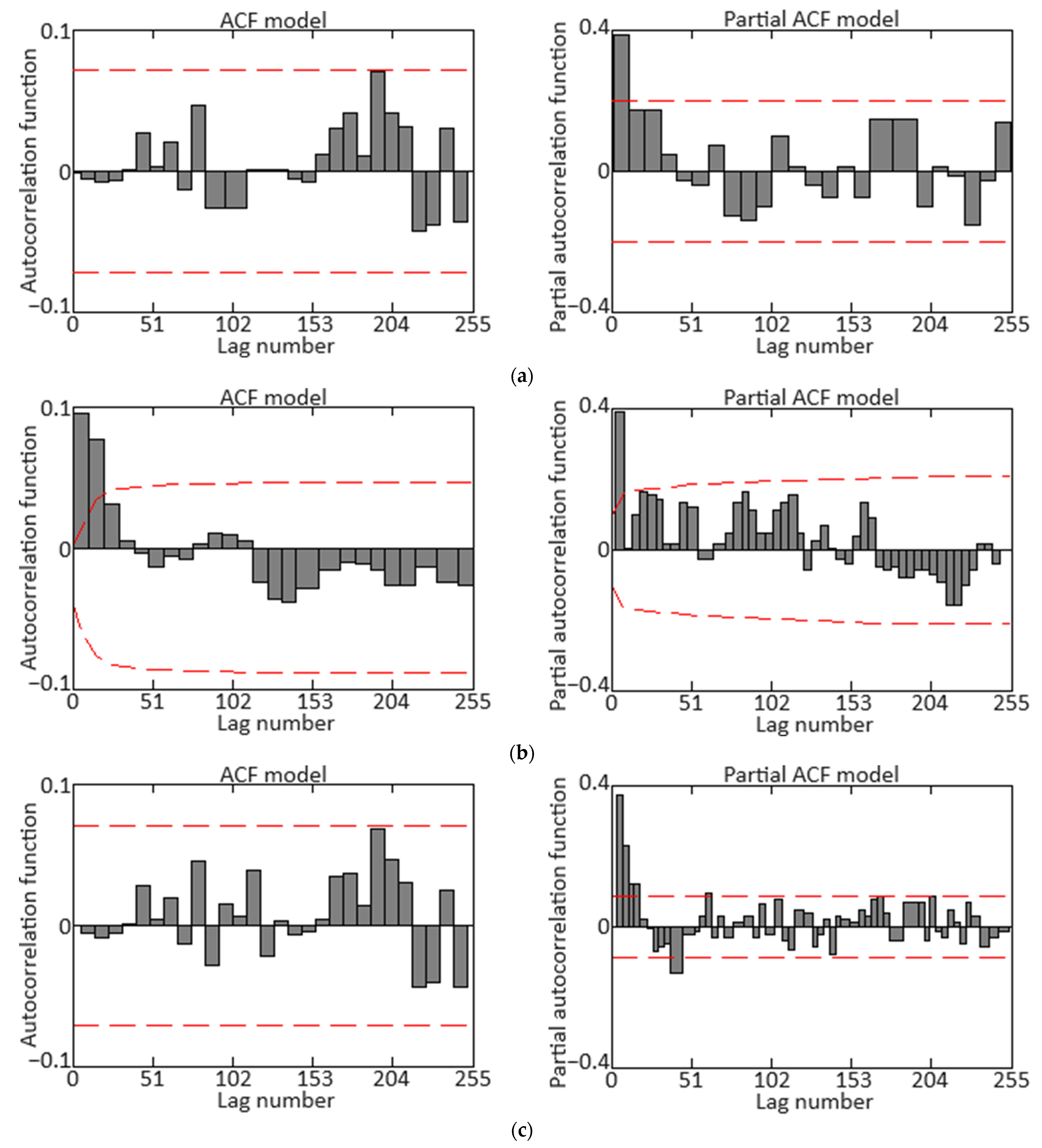
Testing the dataset with ADF and KPSS tests confirmed its non-stationarity. To achieve stationarity, techniques were sequentially applied, including first differencing to remove the trend and seasonal differencing to eliminate seasonality [
50]. The corresponding autocorrelation function (ACF) and partial autocorrelation function (PACF) diagrams are shown in
Figure 6. The final diagrams in
Figure 6c allow for the
SARIMAX model parameters’ following range selections: autoregressive order
p ∈ [0, 7], differencing order
d = 1, moving average order
q ∈ [0, 7], seasonal autoregressive order
P = 1, seasonal differencing order
D = 1, seasonal moving average order
Q = 0, and seasonal period
s = 96.
Clarification: In the context of sensor data registration on board helicopters during flight, the term “seasonality” refers to regular and predictable changes in the data caused by time periods within the year (autumn–winter and spring–summer flights), which must be factored for accurate real-time interpretation and analysis. The impact on the sensor readings for gas temperatures before the compressor turbine in helicopter flight during the autumn–winter and spring–summer periods is linked to variations in the external temperature and pressure conditions, leading to changes in the thermodynamic properties of the air entering the engine [
51,
52,
53]. In this research, the parameters have been adjusted for helicopter flight conditions during the spring–summer period.
In addition to accounting for “seasonality”, the calibration of the predicting system incorporates actual environmental conditions such as temperature, humidity, and atmospheric pressure. These factors significantly influence the sensor data interpretation accuracy, as they affect the engine’s thermodynamic properties and the sensor readings. By integrating these real-time environmental parameters into the calibration process, the system can more precisely adjust for variations and improve the reliability of its predictions under varying flight conditions.
Among all the obtained models, the model with SARIMAX parameters
s = 96, (
p = 6,
d = 1,
q = 5) (
P = 0,
D = 1,
Q = 1) was selected for the data cleaning module’s routine operation. This model was chosen due to its lowest values for the Akaike information criterion (AIC) [
54] and Bayesian information criterion (BIC) [
55] compared to other models, and the residual series (the difference between actual and predicted values) exhibits unbiasedness properties, stationarity, and a lack of autocorrelation.
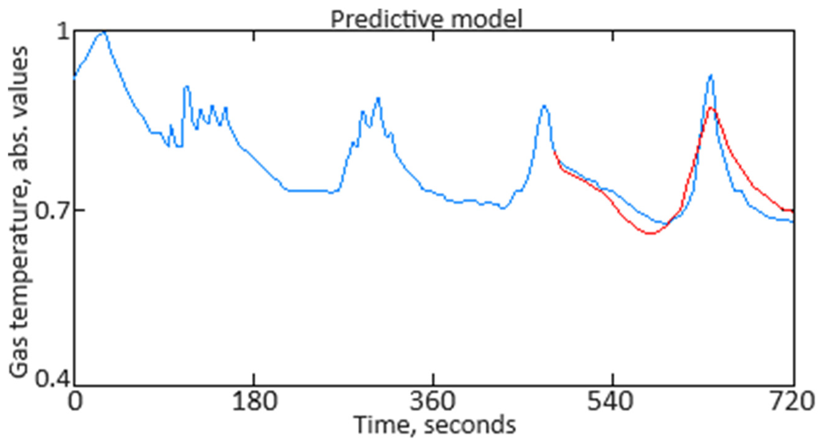
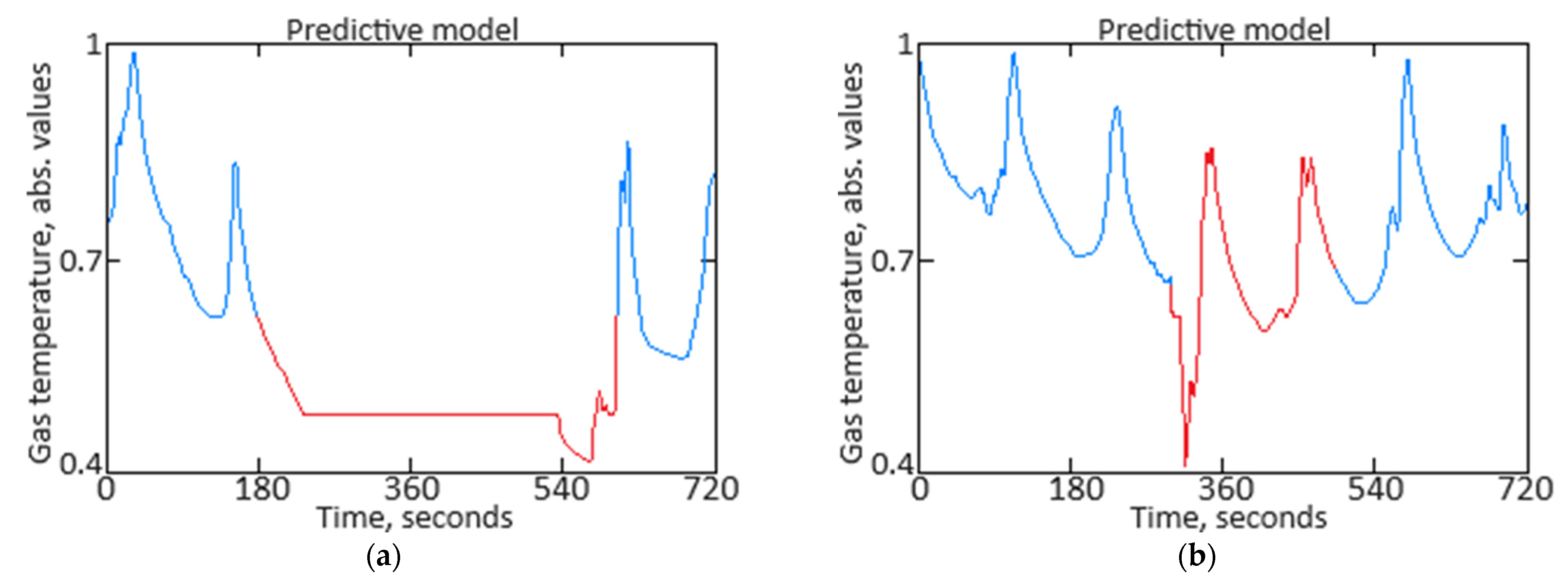
Figure 7 presents a 4 min prediction for helicopter flight, with the prediction error having an
MSE = 0.218%. In
Figure 7, the “blue curve” represents the actual data recorded by the sensor, and the “red curve” represents the predicted data.
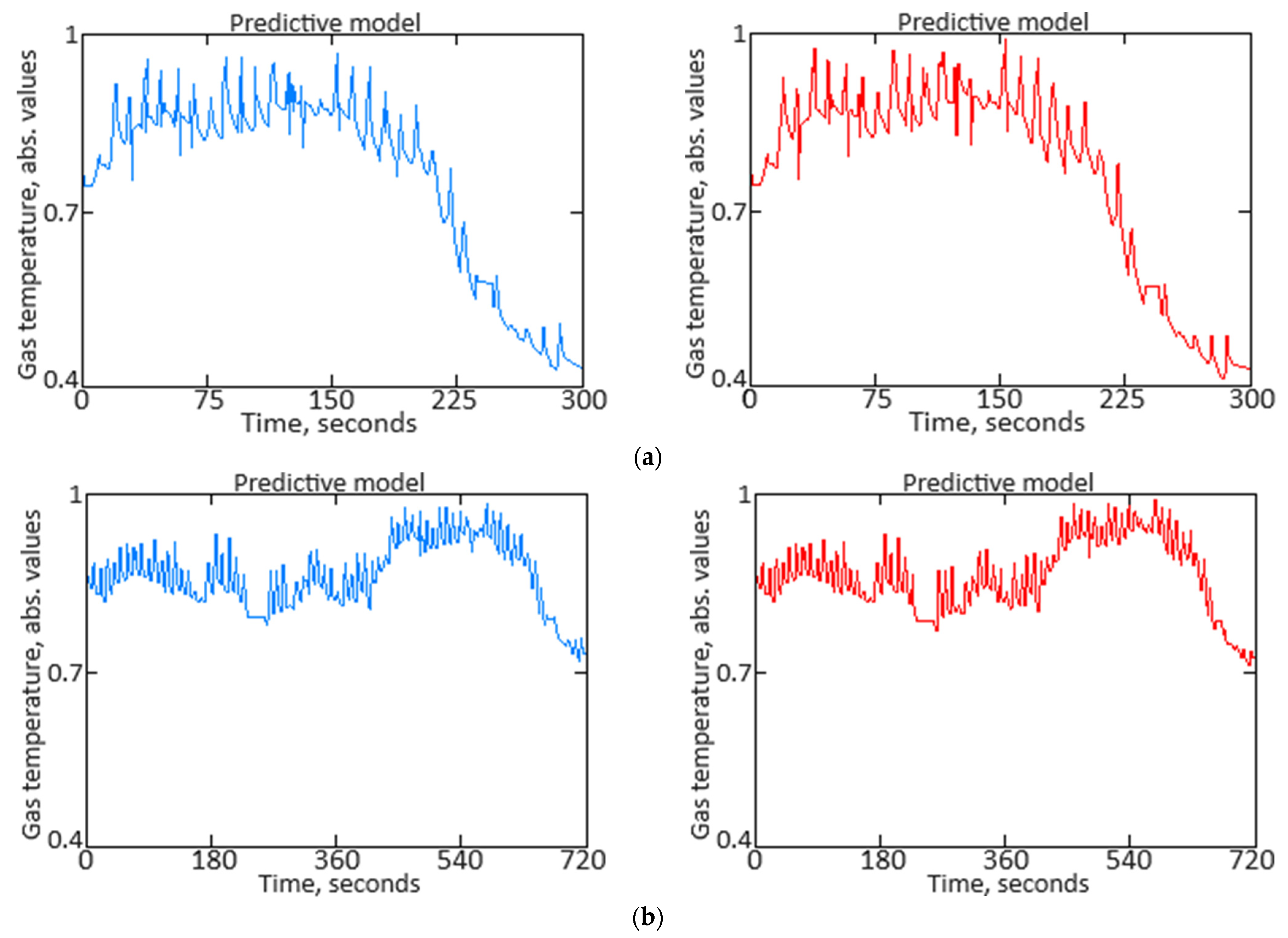
Since the proposed SARIMAX model predicts values for the gas temperature from the TV3-117 aircraft engine’s in front of the compressor turbine sensor with high accuracy, it can be used to replace missing values with plausible synthetic values. Examples of the reconstructor’s performance are shown in
Figure 8. In
Figure 8, the “blue curve” represents the actual data recorded by the sensor, the “red curve” represents restored data, the “red dots” indicate outliers, and the “green dots” represent imputed values.
3.3. Results of Data Anomaly Prediction
Figure 11 illustrates an example of two anomalies detected during the data cleaning module’s simulation, corresponding to two minutes of the TV3-117 aircraft engine gas temperature before the compressor turbine sensor activity under helicopter flight conditions. The first anomaly is a “Top 1 dissonance” found in the test dataset, indicating a temporary malfunction of the sensor. The second anomaly is a “Top 10 dissonance” and points to a rapid decrease in gas temperature before the compressor turbine due to increased airflow speed and changes in external air pressure. In both cases, the detected anomalies require a response from the helicopter’s flight commander (human operator). These anomalies prompt an immediate assessment by the flight commander to determine the appropriate corrective actions or adjustments needed. Such proactive responses help maintain optimal engine performance and ensure operational safety by addressing potential issues before they escalate. The system’s ability to accurately detect and classify anomalies in real time significantly enhances the reliability and responsiveness of the monitoring process.
To better interpret the anomaly detection results, it is important to discuss both healthy and unhealthy conditions in detail. By examining the baseline or normal operational parameters alongside the detected anomalies, one can more accurately assess the system’s performance and sensitivity. Healthy conditions may include stable engine performance with consistent sensor readings and normal gas temperatures before the compressor turbine, indicative of optimal operation. Unhealthy conditions, on the other hand, might involve irregular sensor data, such as sudden temperature drops or fluctuating readings due to sensor malfunctions, increased airflow speeds, or changes in external air pressure.
To perform cross-validation (k-fold cross-validation), the training dataset is partitioned into
k subsets (folds):
D1,
D2, …,
Dk. For each
i-th fold (
i = 1, 2, …,
k), one subset serves as the validation set while the remaining
k − 1 folds are utilized for training. The model is trained on the
k − 1 subsets and assessed on the remaining subset. In each
i-th iteration, the model is trained on data
(and evaluated on data
), where
Subsequently, the metric (in this research,
MSE) is computed on the validation set for each
i-th fold:
where
M(i) represents a model trained on
. Upon completion of all
k iterations, the mean metric value is computed across all folds:
In assessing the effectiveness of the computational experiment, a cross-validation procedure (k-fold cross-validation) was performed. For this, k = 5 equal subsets (folds) of 51 elements each randomly chosen from the training sample. The following metric values were obtained: Metric(k1) = 0.224%, Metric(k2) = 0.228%, Metric(k3) = 0.227%, Metric(k4) = 0.226%, and Metric(k5) = 0.229%. The average metric was calculated as 0.227%, which differs from MSEmin = 0.218% by 3.96%. This indicates that the average value of the metric (mean square error) after cross-validation is close to the MSEmin obtained from one fold (in this case, k3). The 3.96% difference reflects how much the average metric deviates from the best individual result achieved during the cross-validation iterations. The results also suggest that the model demonstrates stability in its predictions across different data subsets (folds), as evidenced by the small difference between the average metric and MSEmin. However, it is crucial to note that the average metric offers a more generalized view of performance across the entire training set, while MSEmin highlights the optimal result obtained from a single data subset. Further analysis could investigate whether additional folds or variations in data distribution might further enhance the model’s accuracy.
3.4. Evaluation of the Effectiveness of the Results Obtained
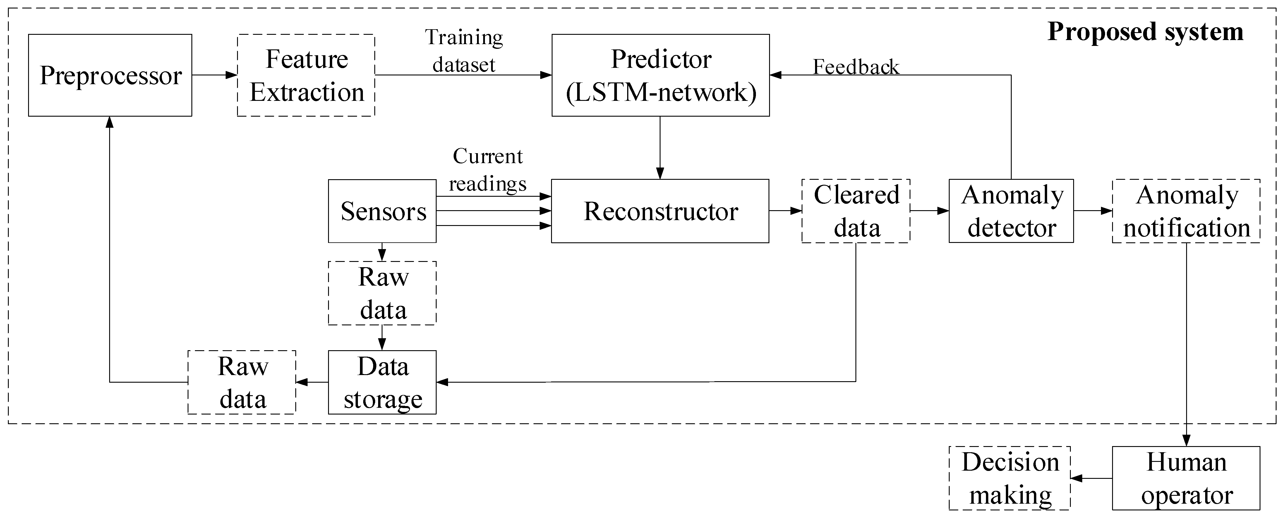
To evaluate the effectiveness [
56,
57,
58,
59,
60] of the proposed neural network system for predicting anomalous data in sensor systems (
Figure 1), various metrics need to be considered, such as mean squared error (
MSE) and mean absolute error (
MAE), which reflect the accuracy in predicting sensor values. The determination coefficient (
R2) shows how well the model explains data variations, while the correctly replaced outlier percentage and the false positive rate demonstrate the effectiveness of the reconstructor and anomaly detector. Additionally, the missed outlier rate and anomaly detection accuracy provide insight into the system’s ability to correctly identify and classify anomalies, while mean response time to anomalies assesses the system’s operational speed. In the context of a system for predicting anomalous data,
Precision reflects the system’s ability to avoid false positives. This is crucial to prevent the operator from being overwhelmed by unnecessary notifications about anomalies that are actually normal data.
Recall indicates how well the system can identify all existing anomalies. The
F1-score is a combined metric that considers both
Precision and
Recall. The ROC curve displays the true positive rate (
TPR) against the false positive rate (
FPR) across various threshold values. These metrics enable a comprehensive evaluation, ensuring the accurate prediction and reliable detection of anomalies in sensor data. The results evaluating the effectiveness of the proposed neural network system for predicting anomalous data in sensor systems are presented in
Table 2. Accordingly, the confusion matrix is given in
Table 3.
True positive (TP) represents the number of cases where the system correctly identified an anomaly, that is, the system classified an event as an anomaly, and it was indeed an anomaly. True negative (TN) represents the number of cases where the system correctly identified data as normal (not an anomaly), that is, the system classified an event as normal, and it was indeed normal. False positive (FP) represents the number of false alarms where the system mistakenly classified normal data as anomalies, that is, the system identified an event as an anomaly, but it was actually not an anomaly. False negative (FN) represents the number of missed anomalies where the system did not recognize an anomaly, that is, the system classified an event as normal, but it was actually an anomaly.
A comparative analysis (
Table 4) was conducted between the developed neural network system (
Figure 1), a neural network system based on an autoassociative neural network (autoencoder) created by the same research team [
2], and a hybrid mathematical model utilizing Runge–Kutta optimization and Bayesian hyperparameter optimization [
31], according to the quality metrics presented in
Table 2.
As shown in
Table 4, the quality metric values for the developed neural network system (
Figure 1) and the neural network system based on the autoassociative neural network (autoencoder) [
2] are approximately equal. This indicates that both systems are interchangeable and can serve as alternatives to one another. The quality metrics for the developed neural network system (
Figure 1) are, on average, up to 20% higher than those of the hybrid mathematical model utilizing Runge–Kutta and Bayesian hyperparameter optimization.
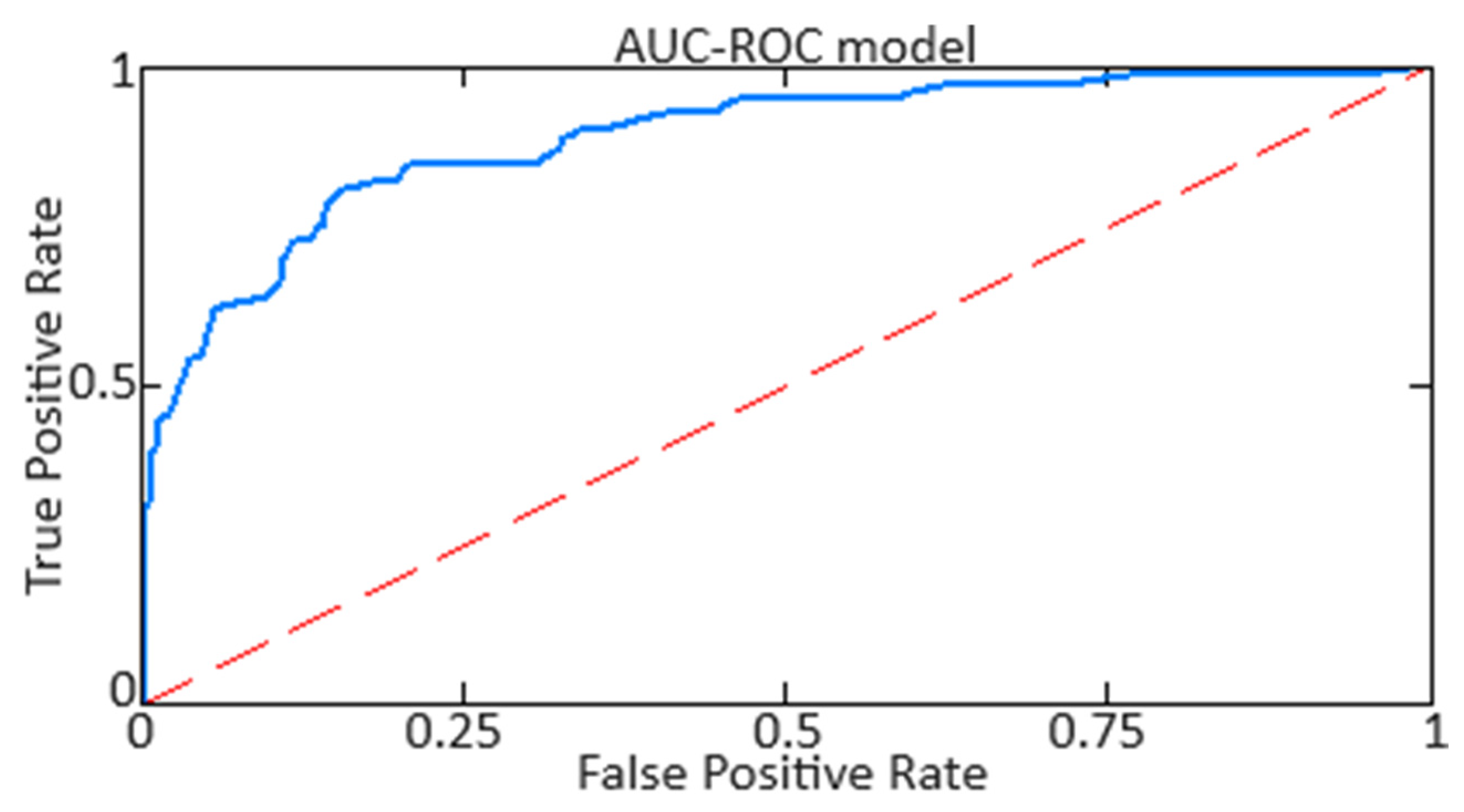
For ROC analysis [
57,
58] across the three approaches (the developed neural network system, the neural network system based on an autoassociative neural network (autoencoder) [
2], and the hybrid mathematical model utilizing Runge–Kutta optimization and Bayesian hyperparameter optimization [
31]), true positive and false positive rates were calculated for each category and technique, followed by the creation of the respective ROC curves. This procedure involved defining a binary classification for each category, isolating it from the others. The ROC analysis results are presented in
Table 5.
Figure 12 distinctly illustrates the variation in the regions beneath the AUC curve for the developed neural network system.
Based on the obtained AUC-ROC metric values, it is noted that the developed neural network system (
Figure 1) and the system based on an autoassociative neural network (autoencoder) [
2] deliver high accuracy with a minimal false alarm rate. The use of the model employing Runge–Kutta and Bayesian hyperparameter optimization [
31] results in lower accuracy and the highest number of false alarms.


 ,
, 


