The conditions set for the unit plot are somewhat arbitrary. The unit plot could have been longer or shorter, or on a steeper or less steep slope. However, conceptually, the unit plot provides the physical model on which the USLE is based, and Equation (2) is designed to account for the effect of geographic variations in climate and soil on soil loss. Equation (3) is designed to account for local variations in slope length, gradient, and cropping practices once the effect of climate and soils has been established at a location.
2.1. The R Factor
Equation (2) deals with the effect of geographic variations in soil and climate on erosion caused by sheet and rill erosion.
R is defined as the average annual value of the product storm kinetic energy (
E) multiplied by the maximum 30-min intensity (
I30):
where
N is the number of valid rainfall events in
Y years. Rain showers of less than 12.5 mm (0.5 in) were omitted in the calculation of
R unless at least 6.25 mm (0.25 in) of rain fell in 15 min. A period of 6 h with less than 1.27 mm (0.05 in) was used as a storm separator. A direct linear relationship between event soil loss from bare fallow and
EI30 for
runoff producing events was demonstrated to exist at Bethany, Missouri by Wischmeier and Smith [
6].
E, storm rainfall energy, was not determined directly, but was usually calculated from rainfall energy–intensity relationships based on the data on raindrop sizes obtained in Washington, DC, by Laws and Parsons [
7]. Initially, in the USLE, the energy per unit quantity of rain or unit kinetic energy was determined from a logarithmic relationship with rainfall intensity, the metric version being:
where
em has units of megajoule per hectare per millimeter of rainfall (MJ ha
−1 mm
−1). The limit of 76 mm h
−1 applied to Equation (5a) resulted from observations that Equation (5a) overpredicted
em when the intensity exceeded that value. In RUSLE [
3], Equation (5) was replaced by:
where as, in RUSLE2 [
8]:
As shown by Nearing [
9], Equation (7) produces higher
em values than Equation (6) below
im = 70 mm h
−1 but both Equations (6) and (7) produce little variation in
em values once
im exceeds 80 mm h
−1.
In reality, storm kinetic energies can vary greatly from the values predicted depending on the synoptic conditions that produce the rainfall [
10]. Although the original conceptual model is based on the understanding that raindrop impact is an important factor in supplying the energy required to cause erosion, in using Equations (5) or (6) or (7), the USLE/RUSLE model ignores the actual variations in rainfall kinetic energy that occur in time and space. In effect, these equations emphasize the influence of rain produced at high intensities in comparison to low-intensity rainfall. This emphasis is enhanced further, because
I30 is highly influenced by high intensities that are associated with the peak rainfall rate that occurs during a rainstorm.
Although
R is assumed not to vary with slope gradient, on low slopes, raindrop impacts tend to be more buffered by water ponded on the surface than on steeper slopes. Consequently, the RUSLE provides an adjustment factor to account for the reduction of
R by ponded water on low slopes [
3]. In the USLE, storms showers of less than 12.5 mm (0.5 in) were omitted in the calculation of
R unless at least 6.25 mm (0.25 in) of rain fell in 15 min. In RUSLE, all storms were considered in the calculation of
R in the western regions of the USA. While it was argued that this had little effect on the value of
R, the reason why storms less than 12.5 mm were originally omitted was that storms less than 12.5 mm were observed by Wischmeier and Smith to often not produce appreciable amounts of runoff and soil loss and, very importantly, the direct linear relationship between event soil loss from bare fallow and
EI30 that was demonstrated to exist at Bethany, Missouri by [
6] was determined from only storms that produced runoff and soil loss. In reality, the USLE/RUSLE model is based on:
where
A1.e = event soil loss (mass/area) from the unit plot, and
Qe (volume/area) is the runoff amount for the event.
Determining
EI30 values for individual storms using
em values requires high-resolution data on the rainfall intensities that occur during a storm. Mapping techniques have been widely used to estimate
R values between locations where such data are available [
1,
2,
3,
11,
12]. However, it should be noted that the amount of soil eroded varies during the year depending on how the erosive rainfall is distributed in time at a location, and how the protective effect of vegetation varies over time. Consequently, in the USLE, not only is
R determined using Equation (4), but also the proportion of
R that occurs during various crop stages is determined in order to deal with the interaction between rain and vegetation on soil loss. In the RUSLE, the proportion of
R that occurs in each half month is used.
2.2. The K Factor
K is the average annual soil loss per unit of
R. Originally,
K values were determined from runoff and soil loss plot data using:
It follows from Equation (8) that
K replaces the regression coefficient that usually associated a direct linear relationship between event soil loss from the unit plot and
EI30. However, Equation (9) ensures that the total soil loss predicted for the set of events used to obtain
K is the same as the total of the soil loss observed for that set of events. That is not always the case when
K is determined as the regression coefficient in the relationship between event soil loss from the unit plot and
EI30.
Given the expense and time necessary to operate appropriate runoff and soil loss plots, methods to predict
K from soil properties were developed later [
13]. Wischmeier et al. [
14] developed a soil erodibility nomograph for determining
K from soil properties. A mathematical approximation was then developed [
2] for those cases where the silt plus fine sand fraction does not exceed 70%:
where
M is the percentage of silt (0.02–0.1 mm) multiplied by the quantity of 100% clay,
OM is the percentage of organic matter,
s is the soil structure code in the US soil classification, and p is the profile permeability class. Auerswald et al. [
15] have developed a more precise equation to predict
K from soil properties.
Often, in the rainfall simulation experiments undertaken to determine
K, artificial rainfall is applied to a plot at about 64 mm hr
−1 under natural antecedent soil–water conditions (dry run), followed by a 30-min simulation 4 h later (wet run), and another 30-min simulation 30 min later (very wet run). This approach results in
K being calculated from:
where
Kd,
Kw, and
Kvw are the respective values for the soil erodibilities associated with the dry, wet, and very wet runs [
16]. The weighting used in Equation (11) reflects a storm frequency distribution for central USA [
17].
In the development of the RUSLE, it was recognized that seasonal variations in soil properties and runoff also resulted in seasonal variations in
K. While the pattern for temporally varying erodibility was well defined at some locations, it was not at others. Examination of the RUSLE temporal soil erodibility equations showed that they worked poorly at 11 locations, and were not applicable in the Western USA [
8].
In RUSLE2 [
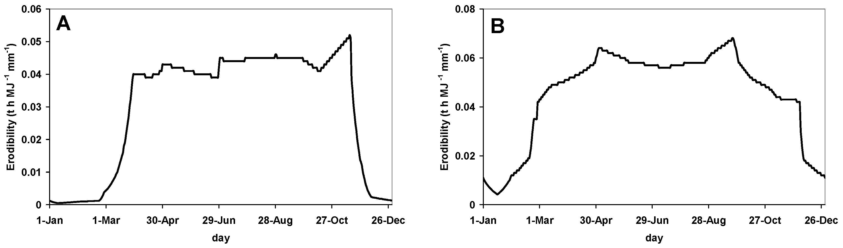
8], a version of the RUSLE that uses a daily time step in the calculation of soil loss in the USA, temporal variations in soil erodibility in the USA are calculated using monthly precipitation and temperature as independent variables. In the Eastern USA:
where
Kj is the average daily soil erodibility factor value for the
jth day,
Kn is the average soil erodibility determined from soil properties,
Tj is the average daily temperature for the
jth day in Farenheit,
Ts is the average daily temperature for the RUSLE2 summer period,
Pj is the average daily precipitation in inches,
Ps is the daily average precipitation for the summer period, and
Ksj is the soil erodibility factor calculated for the
jth day using Equation (12).
Figure 1 shows how
K varies during the year when Equation (12) is applied at Presque Isle, Maine (ME), and Bethany, Missouri (MO) in the USA.
It is important to note that the approach results in the average annual value for soil erodibility calculated from soil properties vary geographically with climate in the USA. However, Equation (12) does not describe increased soil erodibility during or immediately after soil thawing, or work well in the Western USA. In the Western USA,
Ps and
Ts values are set to the values at Columbia, Missouri to give:
This equation estimates increased K values at locations where more precipitation or cooler summers create wetter soil conditions with an increased likelihood of runoff occurring. The applicability of this approach outside the USA is untested.
In many cases where the USLE/RUSLE model has been applied either in the USA or outside the USA, soil erodibilty values are assumed to remain constant with time. Consequently, the USLE/RUSLE model has been frequently applied either in the USA or outside the USA without recognizing that the values of
K generated by Equation (10) need to be adjusted for the climate at the location being considered when that location is outside the central USA. However, other equations for calculating
K from soil properties have been developed for places such as Hawaii [
19], Australia [
20], Sicily [
21], and elsewhere. Panagos et al. [
22] applied Equation (10) with an adjustment for stone cover throughout Europe.
2.3. Alternatives to EI30
The USLE model was designed to predict long-term soil loss. However, given that the USLE is based on Equation (8), it can be applied to predicting soil losses on a shorter time scale. Tiwari et al. [
23] observed that the RUSLE overpredicts small average annual soil losses and underpredicts high average annual soil losses in the USA. Although event soil loss from bare fallow was shown to be directly related with event
EI30 at Bethany, Missouri by Wischmeier [
6], that is not the case for all the geographic locations in the USA. Foster et al. [
24] observed that an event erosivity index that had a provision to account for both raindrop and flow-driven erosion separately was better than the
EI30 index. Earlier, Williams [
25] had proposed the Modified Universal Soil Loss Equation (MUSLE):
where
Re is the event erosivity index,
Qve is the volume of runoff for the event in m
3, and
qpe is the peak flow rate for the event in m
3 s
−1. The focus of the MUSLE is sediment yield from watersheds, where Williams et al. perceived flow-driven erosion to be dominant. It should be noted that the value of 11.8 was empirically derived for the specific conditions used by Williams. It does not necessarily apply to all areas where flow-driven erosion is dominant.
It seems that the MUSLE influenced Onstad and Foster [
26] to propose an erosivity index which included a provision to account for both raindrop and flow-driven erosion separately:
where
Qe1 is the event runoff amount from the unit plot, and
α and
β are coefficients that add together to make 1.0, and adjust for variations in the relative capacities of rain and runoff to cause erosion. Assumptions have to be made about the relative effects raindrop-driven and flow-driven erosion in order to set the values of
α and
β when predicting soil loss. Onstad and Foster [
26] used
α =
β = 0.5 and adjusted the value of χ so that it resulted in the average annual average of the value produced by Equation (15) being equal to value of
R calculated using
EI30 alone. Other indices such as:
where
DA is drainage area expressed in ha, and
b4–
b6 are user-selected coefficients that are used as alternatives to
EI30 in APEX [
27]. APEX expanded the number of the erosivity index options available in EPIC [
28]. Williams et al. [
28] also developed an alternative equation to the one used in the USLE to calculate
K. When used to model soil loss, Equations (14), (15), (16a)–(16e) all use USLE/RUSLE
K values, even though
K has units of soil loss per unit of
EI30. Equation (15) is the only one that can use USLE/RUSLE
Ks legitimately, because χ is set so that the average annual average of the value produced by Equation (15) was equal to the value of
R calculated using
EI30. USLE/RUSLE
Ks have units of soil loss per unit
EI30, and that fact needs to be respected when they are used in soil loss prediction models.
Another index that can be considered as an alternative to
EI30 is the
QEA index. This index is calculated by summing the product of the runoff rate (
Q) and the rainfall kinetic energy flux (
EA) during a rainstorm. Runoff is an important factor in determining event soil loss, not just because of flow-driven erosion, but also because the soil loss from runoff and soil loss plots is directly related to the product of runoff and sediment concentration, as well as the mass of soil per unit of runoff. The
QEA index is based on the concept that sediment concentration varies with the rainfall kinetic flux that is applied when runoff occurs. Kinnell et al. [
29] showed that the
QEA index estimated event soil losses from a bare fallow plot at Holly Springs, Mississippi (MS), better than
EI30. They also showed that the excess rainfall rate (
Ix), which can be determined assuming that the infiltration rate of the soil is constant during the rainstorm, could be used as a surrogate for
Q. The coefficients of determination (
r2) for the two bare fallow plots at Holly Springs were 0.5173, 0.6429, and 0.6264 on plot C5, and 0.4613, 0.5758, and 0.5758 on plot C7 for
EI30,
QEA, and
IxEA respectively. The lack of available data on runoff rates and rain intensities during rainstorms at other locations prevented examination of the applicability of
QEA and
IXEA indices at other locations in the USA.
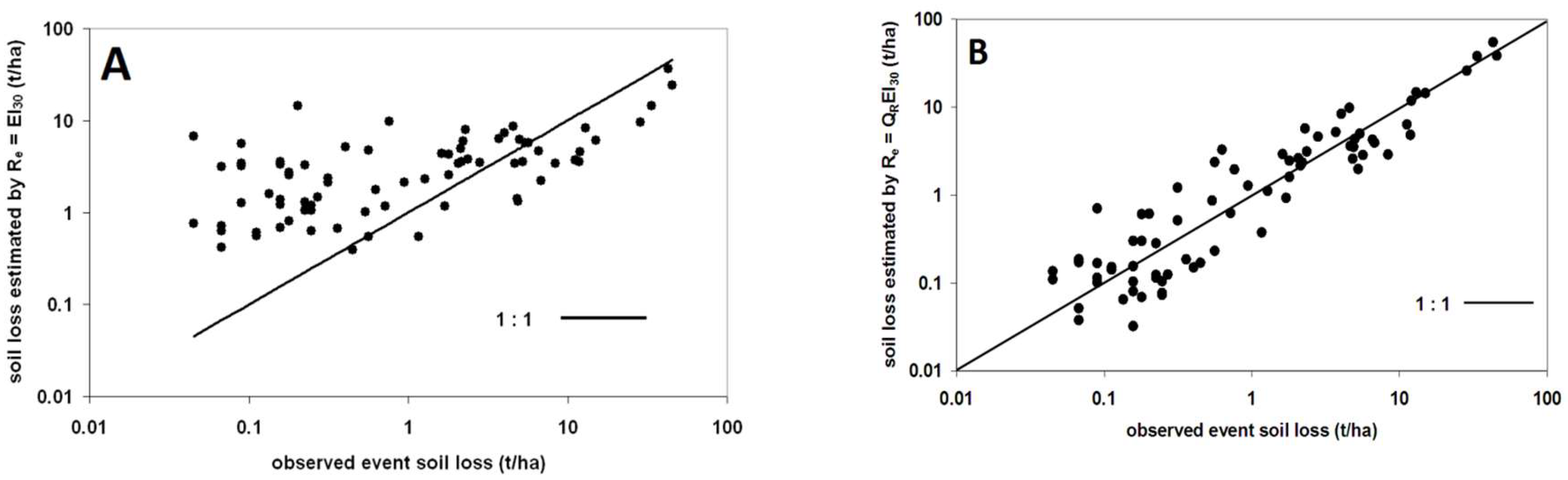
As noted above, runoff is an important factor in determining event soil loss, because soil loss from runoff and soil loss plots is directly related to the product of runoff and sediment concentration (the mass of soil per unit of runoff). When the USLE/RUSLE model is considered in terms of the product of runoff and sediment concentration, it can be seen that the model is based on assumption that the sediment concentration associated with the unit plot varies inversely with runoff:
Kinnell and Risse [
30] observed that for the bare fallow runoff and soil loss plots in the USLE database, sediment concentration was better related to
EI30 per unit quantity of
rain than
EI30 per unit quantity of
runoff. As a result, soil loss for the unit plot predicted by the USLE-M, the name given to the model based on this result, is given by:
where
QRe.1 is the runoff ratio for the event from the unit plot, and
KUM is the soil erodibility for the event, which has a different value from
K, because the event erosivity index is equal to
QR1EI30, not to
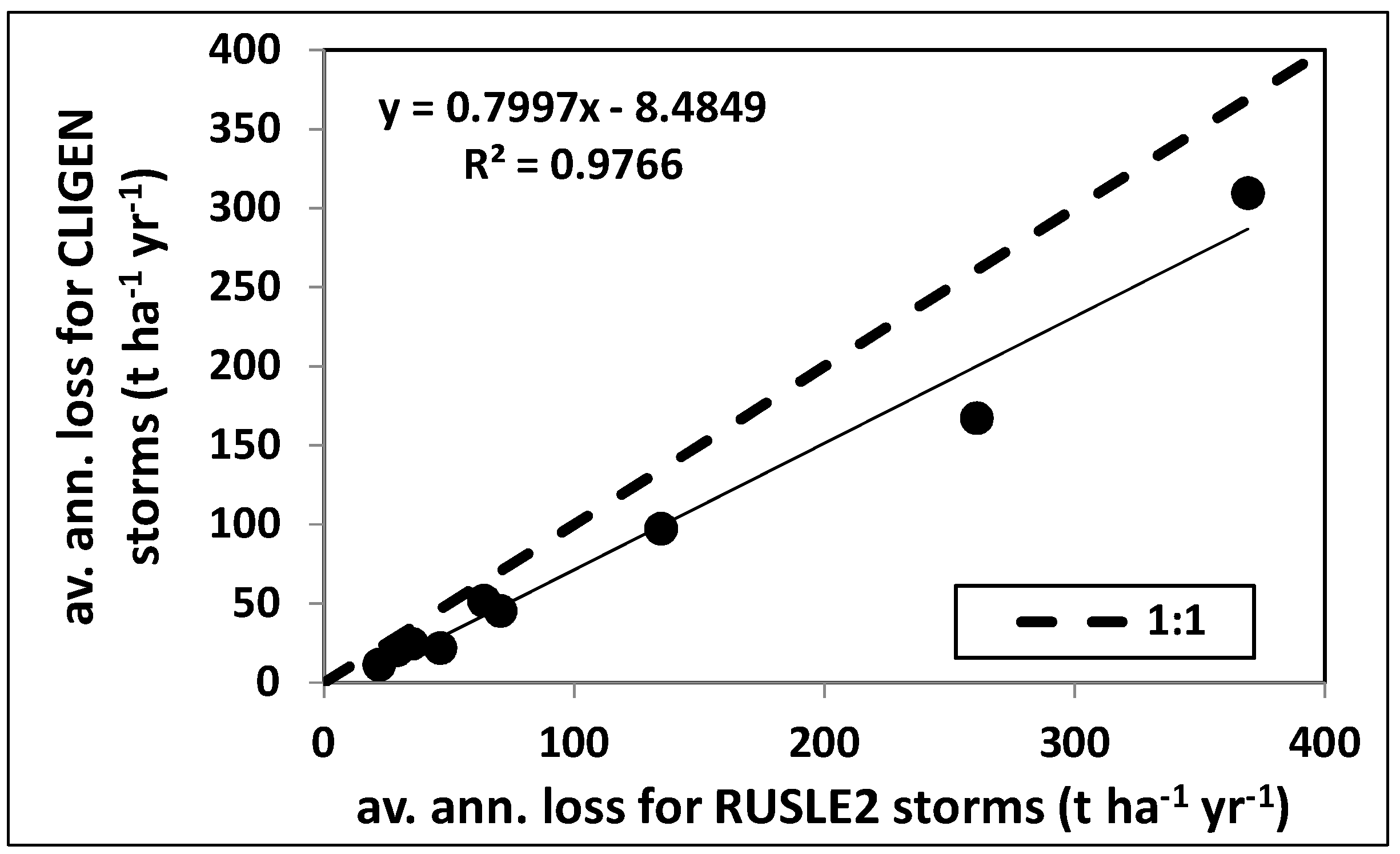
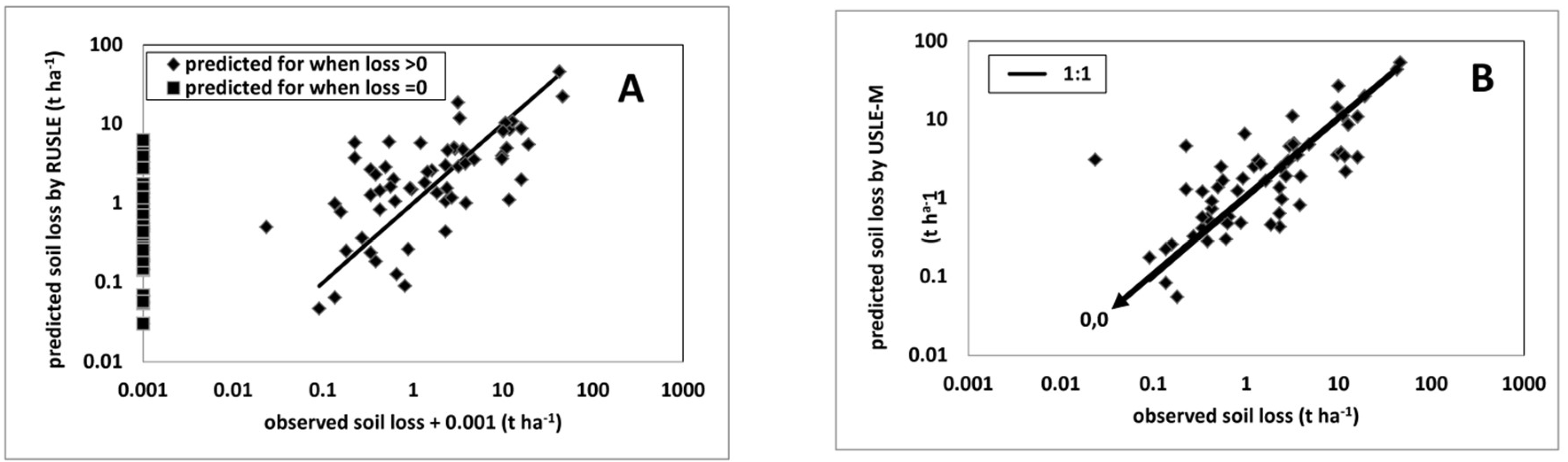
EI30. An example of the improvement in using Equation (18) in place of Equation (8) is shown in
Figure 2 when runoff amounts are known, and:
Obviously, the improvement is not as great when runoff is predicted rather than measured. However, the lack of precision provided by runoff prediction methods will influence the ability of any model that includes runoff as a factor in the prediction of soil loss. Physically-based rainfall erosion models such as WEPP [
4] use runoff as a factor in the prediction of soil loss from both rill and interrill areas.
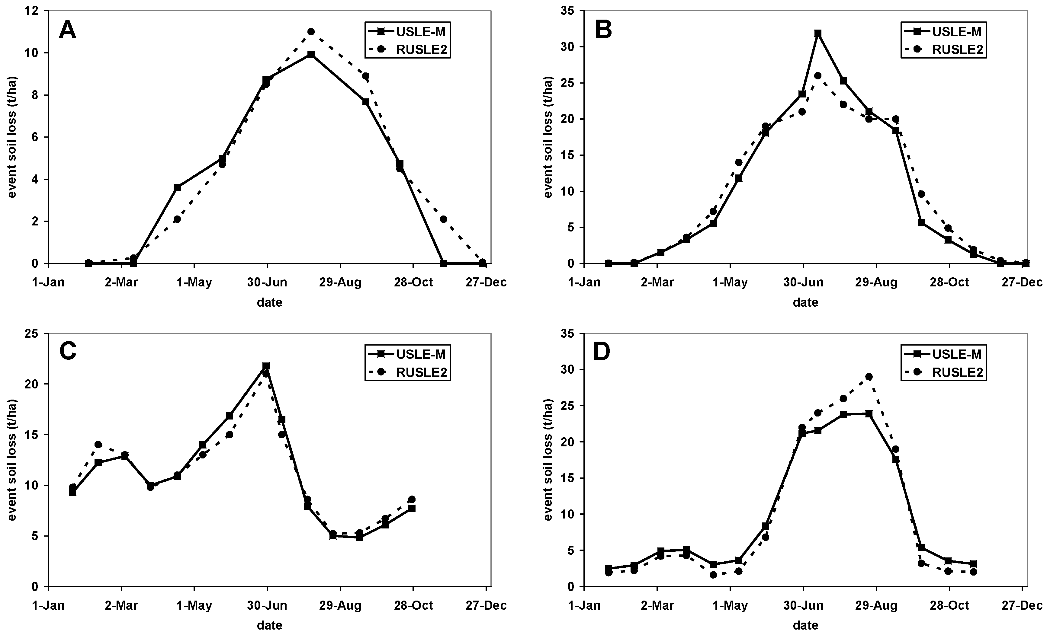
Equation (18) can be rewritten as:
It follows from Equation (20) that the product of
QRe.1 KUM provides runoff-influenced erodibility values that can used as alternatives to the values of
Kj that are normally used in RUSLE2. RUSLE2 has a facility to produce a series of representative storms with associated runoff amounts calculated using the Curve Number (
CN) method [
32], with empirical equations that vary the values of
CN in association with both soil moisture and rainfall intensity [
33].
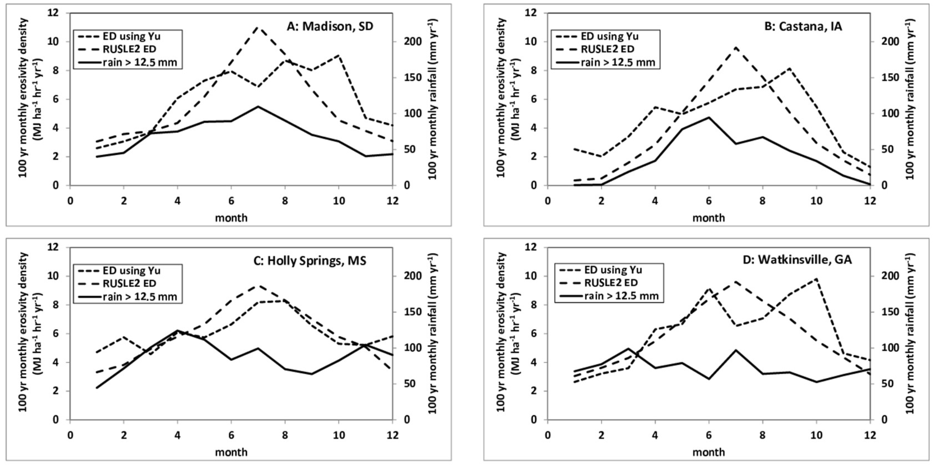
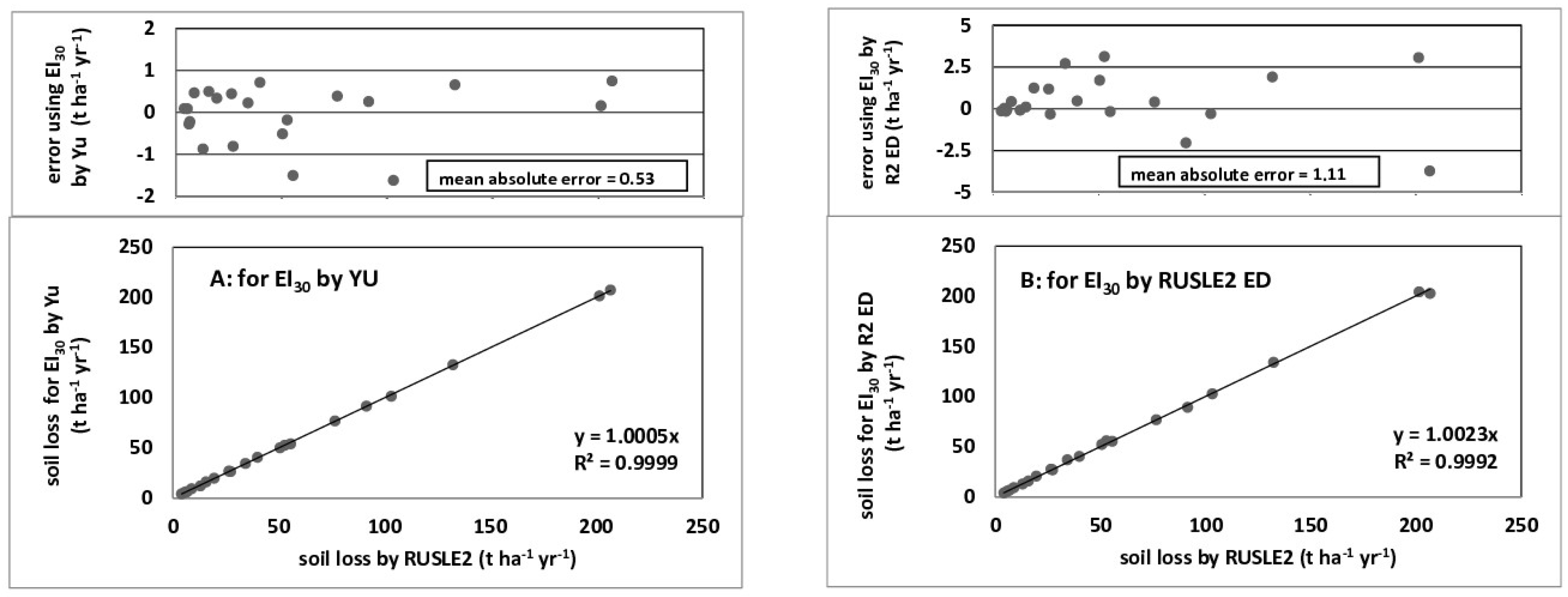
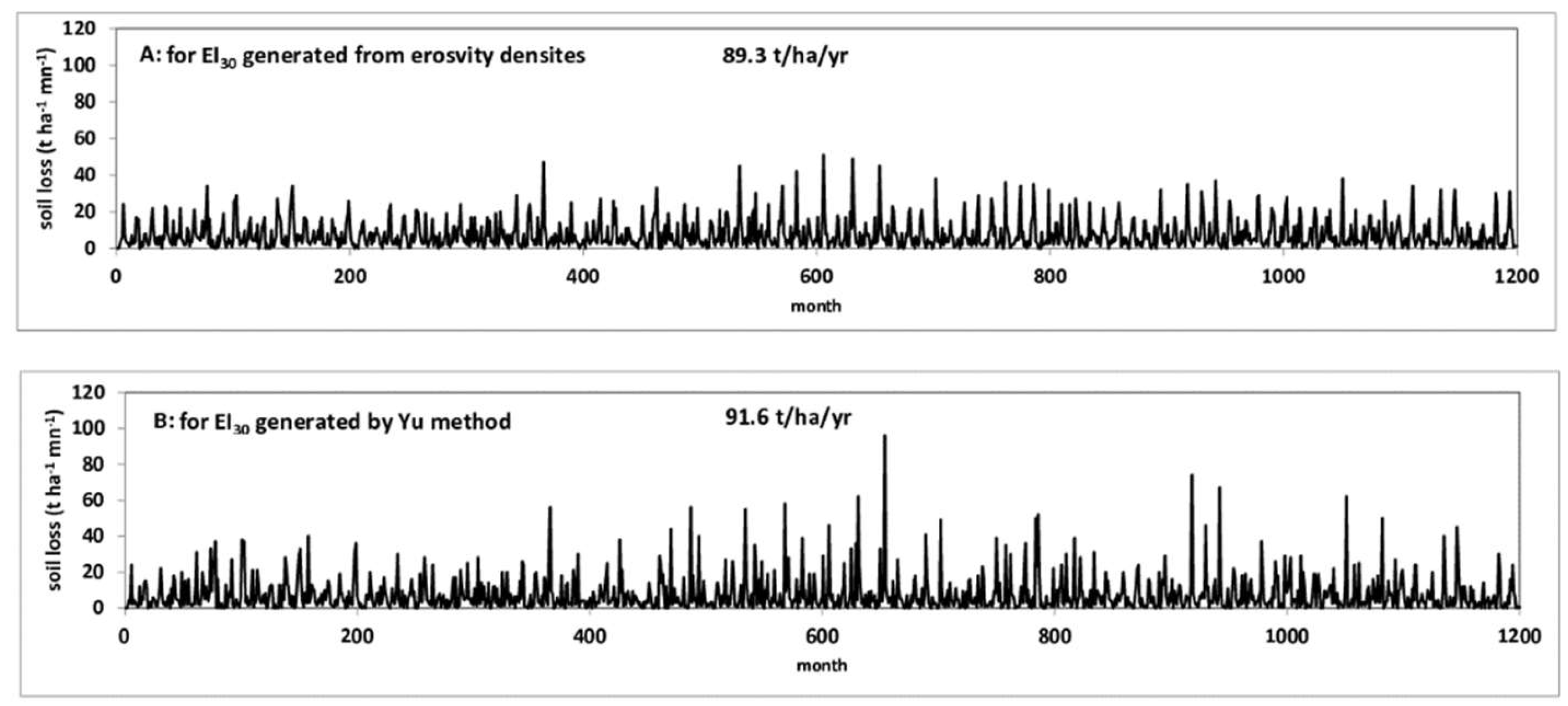
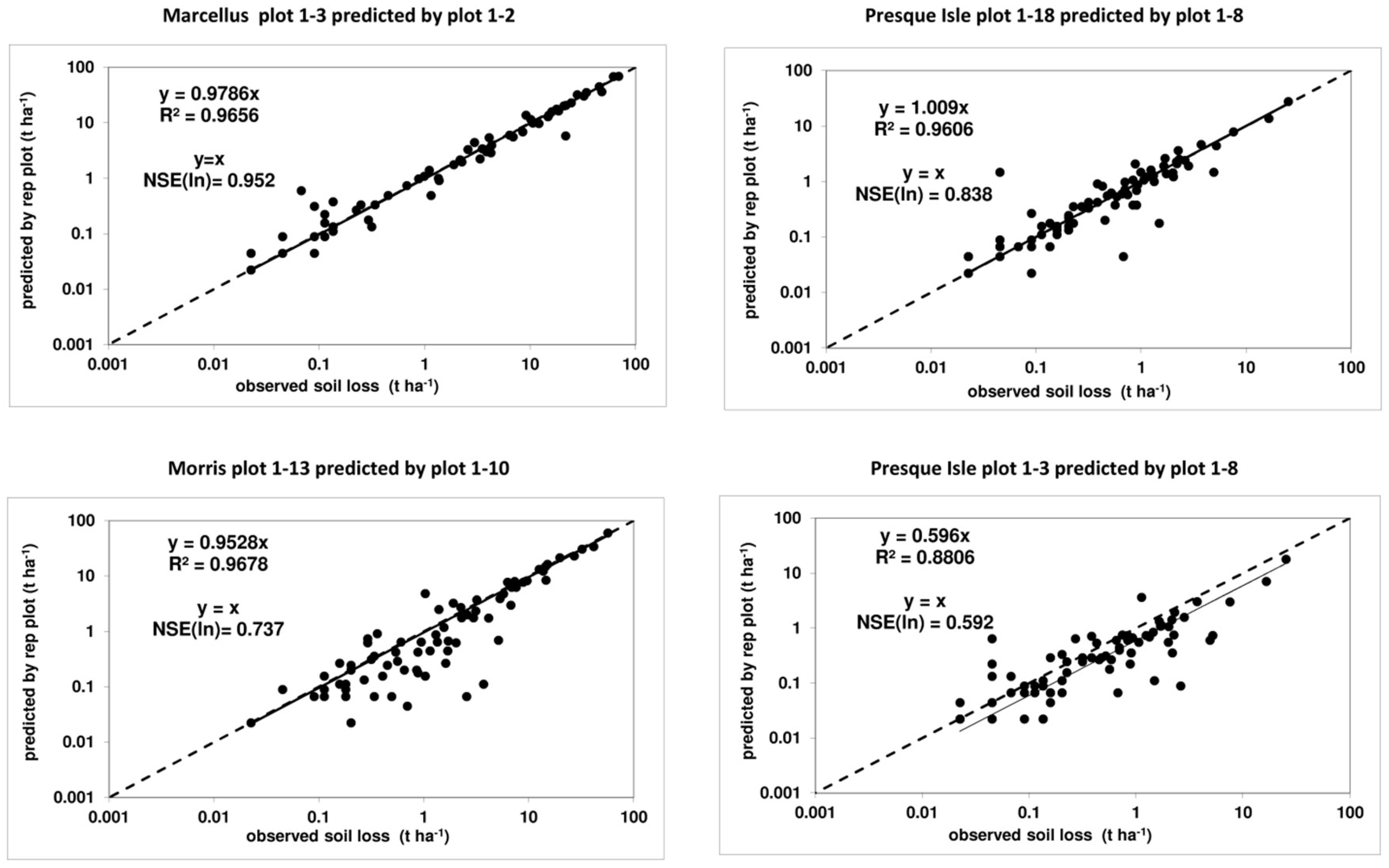
Figure 3 shows how the two different approaches to determining erodibilities for the representative storms compare with each other at four locations in the USA.
The assumption that
Ae.1 is directly related to
QR1EI30 is challenged by data collected from bare fallow runoff and soil loss plots at the Sparacia site in Sicily, Italy. Bagarello et al. [
34] observed that event soil losses from the unit plot varied with
QR1EI30 to a power of 1.61. Subsequent analysis reduced the power to 1.47 [
35] and, based on this result, they proposed the model that they called the USLE-MM.
where
b1 > 1 and
KUMM is the soil erodibility factor when (
QREI30)
b1 is used in place of
QREI30. For the Masse site in Umbria, Italy, they observed the power to be 1.16 [
36]. Bagarello et al. [
36] provided no substantiated physical reason why the power of the
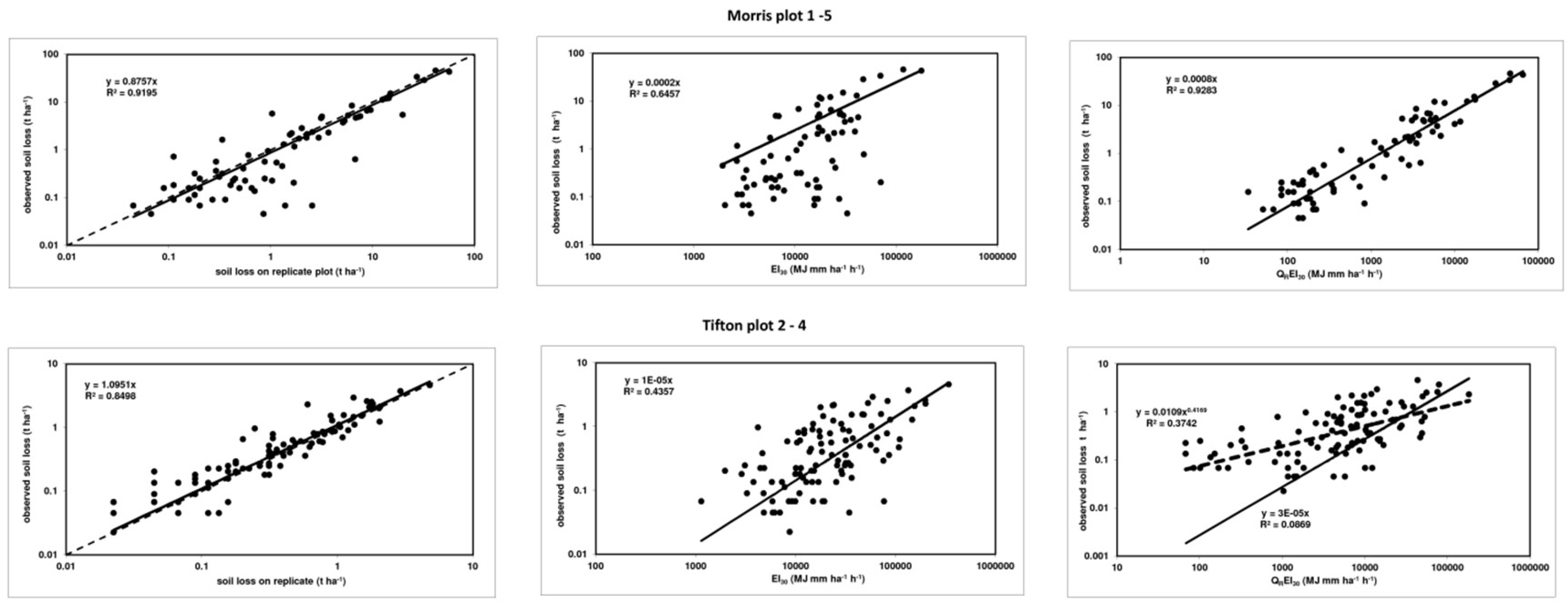
QR1EI30 index should be greater than 1.0 at these two locations. For the USA data used by Kinnell and Risse [
30], powers were mainly grouped within the range of 0.73 to 1.05 [
37]. The exceptions were plots 1–2 at Tifton, Georgia, where the power was 0.419. No physical explanation is available for these values.
In the USLE-MM,
KUMM is given by:
Given the different values of
b1, the units for the soil erodibility factor
KUMM vary between the various locations. However, Kinnell [
37] showed that it is possible to separate the erodibility effect from the effect of
b1 on
KUMM by using:
where:
It follows from Equations (19), (22) and (24) that:
The generalized form of Equation (23) is:
where
X is an erosivity index, and:
Equation (27) ensures that the total sum of the predicted losses is equal to the total sum of the observed losses for the set of events considered. Kinnell [
37] observed that when
X =
QREI30:
Bagarello et al. [
38] suggested that the event erosivity factor could generally expressed as the product of (
QR)
b3 and (
EI30)
b4, where
b3 and
b4 are empirical coefficients that may be different from each other. The case where
b3 ≠ 1 and
b4 = 1 was named USLE-MB. At the Sparacia site in South Italy, they observed
b3 = 1.45. Using this value of
b3 together with site-specific equations for slope length and gradient produced predictions with a Nash–Sutcliffe model efficiency index [
39] of 0.73, which was marginally better than the value of 0.72 produced by Di Stefano et al. [
40] using the USLE-M.
The model proposed by Bagarello [
38] ignored that the values of
b3 varied from 1.43 to 1.76 as slope length varied from 11 m to 44 m on the 14.9% slope at Sparacia. The approach adopted by Bagarello et al. ([
35,
38]) ignores that the USLE-M is based on the concept that sediment discharge from runoff and soil loss plots is given by the product of the amount of water discharged during a rainstorm, and the bulk sediment concentration of the sediment in that water. The
QREI30 index is in fact the product of the runoff rate, the energy per unit quantity of rain during the storm, and
I30. In this scheme, the bulk sediment concentration of the sediment for the storm is empirically related to the product of the energy per unit quantity of rain during the storm and
I30. It can be argued that on the 14.9% slope at Sparacia, sediment concentrations varied with runoff rate to powers that varied from 0.43 to 0.76 as the slope length varied from 11 m to 44 m.
It should also be noted the
EI30 per unit quantity of rain during the storm is termed “erosivity density” in RUSLE2 [
8]. Consequently, the USLE-M equation for the soil loss produced by a storm on the unit plot can be written as:
where
Qe is event runoff, and
εe is the erosivity density for the storm. In this situation, the product of the erosivity density,
I30 and
KUM, focuses on the effects of rain and soil on sediment concentration. For the USLE-MB:
where
KMB is the relevant soil erodibility factor value [
38].
2.4. The L Factor
Although the 22.1-m slope length was commonly used in the experiments upon which the USLE was based, soil loss data were obtained for other lengths. As noted above, Zingg [
5] published the results of a comprehensive study on the effects of slope steepness and slope length on soil loss from runoff and soil loss plots. Later, over 500 plot years of data for plots up to 190 m in length were analyzed [
6], leading to the equation:
where
λ is the distance in meters from the onset of runoff to a point where deposition occurs or runoff enters a channel. In the USLE,
m varies with slope gradient (
s) [
1,
2]:
In the RUSLE, the variation in
m is dependent on the degree of rilling that occurs on the eroding surface:
where
β is the ratio of rill to interrill erosion for the soil being eroding. For soils moderately susceptible to both rill and interrill erosion [
3]:
When a situation where the soil is highly susceptible to rilling occurs, the values of
β applicable to determining
m are recommended to be twice those obtained using Equation (34), whereas for the values of
β for situations where rilling is slight, half the values obtained using Equation (34) should be used [
3]. Generally, Equation (31) should not be used when
λ exceeds about 330 m [
3].
In developing the USLE, it was assumed that the runoff amount (volume per unit area) from runoff and soil loss plots was not affected by the slope length and gradient. As a consequence, the product of
λ and runoff amount gives the volume of runoff discharged per unit width of the plot, and the slope length factor can be perceived to focus on the effect of volume of runoff increasing with slope length. Given that stream power is directly related to flow discharge and slope gradient, and stream power is the rate of energy dissipation against the surface over which the water flows, there is a physical basis to the USLE/RUSLE slope length factor [
41].
An equation to estimate soil loss from a segment on a hillslope was developed by Foster and Wischmeier [
42]:
where the subscript
i represents the
ith segment from the top of the slope. This equation represents the net result of calculating the difference in the mass of soil discharged from the two relevant slope lengths, and then dividing that result by the product of the difference in the slope lengths and 22.1 to determine the soil loss for the segment. A slope length factor for grid cells that is consistent with the concept that the slope length factor focuses on the flow of surface water through the cell and Equation (35) was developed by Desmet and Govers [
43]:
where χ
upslope.j,j is the area upslope of cell
i,j that contributes to the surface water flowing though the cell, and
D is the size of the cell. In Equation (36), the effective slope length to the top of the cell is given by dividing the upslope area that contributes to the flow into the cell by the width of the boundary over which the surface water flows. Likewise, the effective slope length to the bottom of the cell is given by dividing the upslope area that contributes to the flow out of the cell by the width of the boundary over which the surface water flows. Given that Equation (31) should not be applied when
λ exceeds 330 m [
3], that effective slope length should not exceed 330 m. This restriction is frequently ignored in modeling erosion using USLE-based models with Geographic Information Systems in catchments or watersheds. Regardless of the upslope area, the effective slope length should be terminated when an area of concentrated flow is reached. Also, in the USLE and the RUSLE, the effective slope length should be terminated when sediment deposition occurs, but RUSLE2 provides routines that handle deposition
As noted above, there is a physical basis to the USLE/RUSLE slope length factor when the runoff amount (volume per unit area) does not vary with slope length. There are cases where the runoff amount increase with slope length [
6] or decrease with slope length [
44]. Arguably, the value of λ should be adjusted to account for spatial variations in the generation of runoff. A possible approach could be to use the ratio of the runoff amount produced on the bare fallow focus area (
Q) to the runoff amount associated with the unit plot (
Q1) to give:
2.6. The C Factor
Basically, the
C factor is the ratio between the soil loss from a vegetated area and a bare fallow area on the same soil, slope gradient, and slope length for the same set of rainfall events. Initially, it was determined from long-term measurements of soil loss from cropped and bare fallow plots, and consequently, considerable amounts of time were required to obtain average annual values for the wide variety of crops and climates that existed in the USA. Recognition of the fact that average annual values of
C resulted from the interplay between the erosiveness of rainfall and the protective effect of vegetative cover as they vary during the year led to a more versatile approach. Initially, the approach was based on the periods associated with five crop stages and the ratios of the soil losses from cropped plots to the corresponding losses from continuous fallow calculated to give the effective
C factor value for that stage for each particular crop [
1]. Later, Mutchler et al. [
46] used the concept that the effect of cropping on soil loss could be associated with a number of subfactors. In the RUSLE, half-monthly periods are used instead of crop stage periods with subfactors for prior land use, crop canopy, surface cover, surface roughness, and soil moisture used to determine how crops and crop management affect soil loss during the year in 140 different climate zones in the USA [
3]. The distribution of erosive stress during the year influences the average annual value of
C, and each of the 140 climate zones has a different temporal distribution of erosive stress. The approach to determining
C for any given half-month involves multiplying the half-monthly proportion of the annual erosivity by the half-monthly value of the soil loss ratio (
SLR):
where
PLU is the prior land-use subfactor,
CC is the canopy cover subfactor,
SC is the surface cover subfactor,
SR is the soil roughness subfactor, and
SM is the soil moisture subfactor. Renard et al. [
3] provided equations for determining each of these subfactors. Although the procedures described by Renard et al. [
3] stem from scientific research undertaken after the 1960s, some assumptions and approximations had to be used to provide a working model to deal with these effects. In RUSLE2, modeling is done on a daily rather than half-monthly basis [
8] as a means of gaining more flexibility in dealing with the manner in which crops are cultivated and grown. Extensive databases are required to store the information needed to deal with the effects associated with the numerous agricultural practices that exist in the USA and elsewhere. Frequently, in modeling erosion using USLE-based models with Geographic Information Systems in catchments or watersheds, the intra-annual variability of soil cover conditions in arable land is neglected [
47].


