3.1. Validation by Experimental Results
Further, the evaluation of the damping ratio of the system is needed. The value ξ = 0.003 is used in Reference [
14] (See page 251, Equation (28).), but here, Figure 9 of Reference [
9] is used in the simulations.
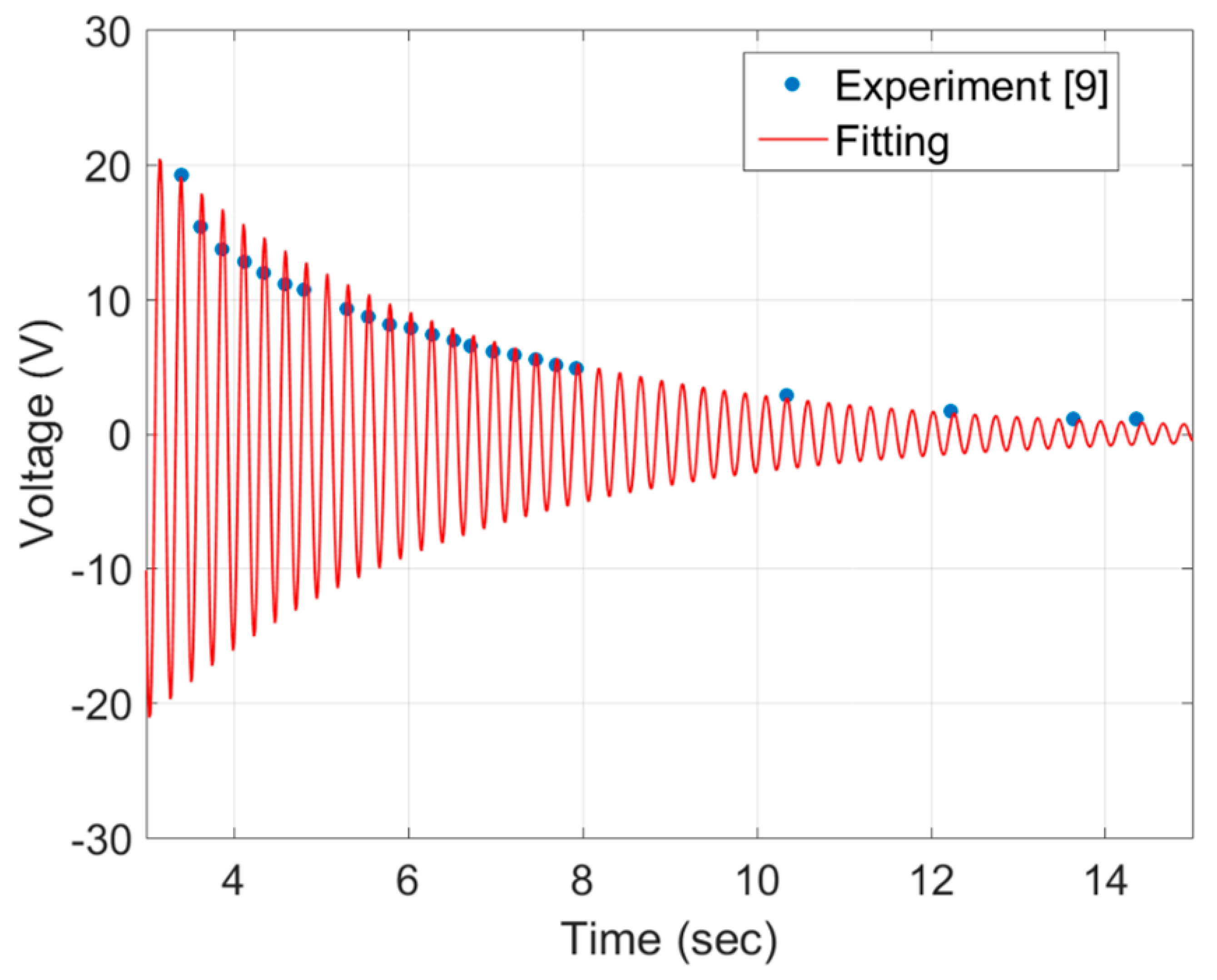
Figure 4 presents the evaluation of the damping ratio of the system from the measured impulse response of the beam with electrodes in an open circuit [
9]. The estimated value by using the tip values of voltage presented in
Figure 4 are ξ = 0.0109 and
f = 4.17 (1/s).
The most important features of the numerical results and its comparison with the experimental results of Sirohi and Mahadik [
9] is presented in
Table 3. The results of the simulation of the system (of which the physical property is given in
Table 1) with the aerodynamic coefficient given in
Table 2 are summarized in
Table 3. As shown in the calculation of natural frequency, the relative error of the used method is less than 2 percent while the relative error of the Galerkin procedure by Abdelkefi et al. [
14] is more than 45 percent (See Table 2 in Reference [
14].). They found that the angular velocity for the first mode is 38.176 which resulted in 6.076 Hz in frequency. Since the results of the approximate method have less error in comparison with the finite element method, this difference comes from the application of the first order Rayleigh–Ritz method instead of the higher-order modal method or Galerkin method used in Reference [
14], which affect the difference in natural frequency and effective mass of the system.
Also, it is revealed in
Table 3 that the onset of galloping (with the aerodynamic coefficients of
Table 2) for the system based on the Equation (42) is predicted at 22.79 m/s. The value at load resistance (0.7 MΩ) is 40.9455 m/s, while for 9.5 mph (4.25 m/s), the value of 30 Volts (which is approximately a 2-mm tip deflection) is seen (See Figure 8 of Reference [
9], and consider mph = 0.44704 m/s.). One conclusion of this paradigm could be that observed motion, in that case, is not a real galloping, and the coefficients of
Table 2 are not recommended. Although the authors of References [
13,
14] solved this paradigm by using artificial values for the system damping ratio, they exposed unrealistic results for tip displacement in the next step. The aerodynamic coefficient values which fit the experimental results of Reference [
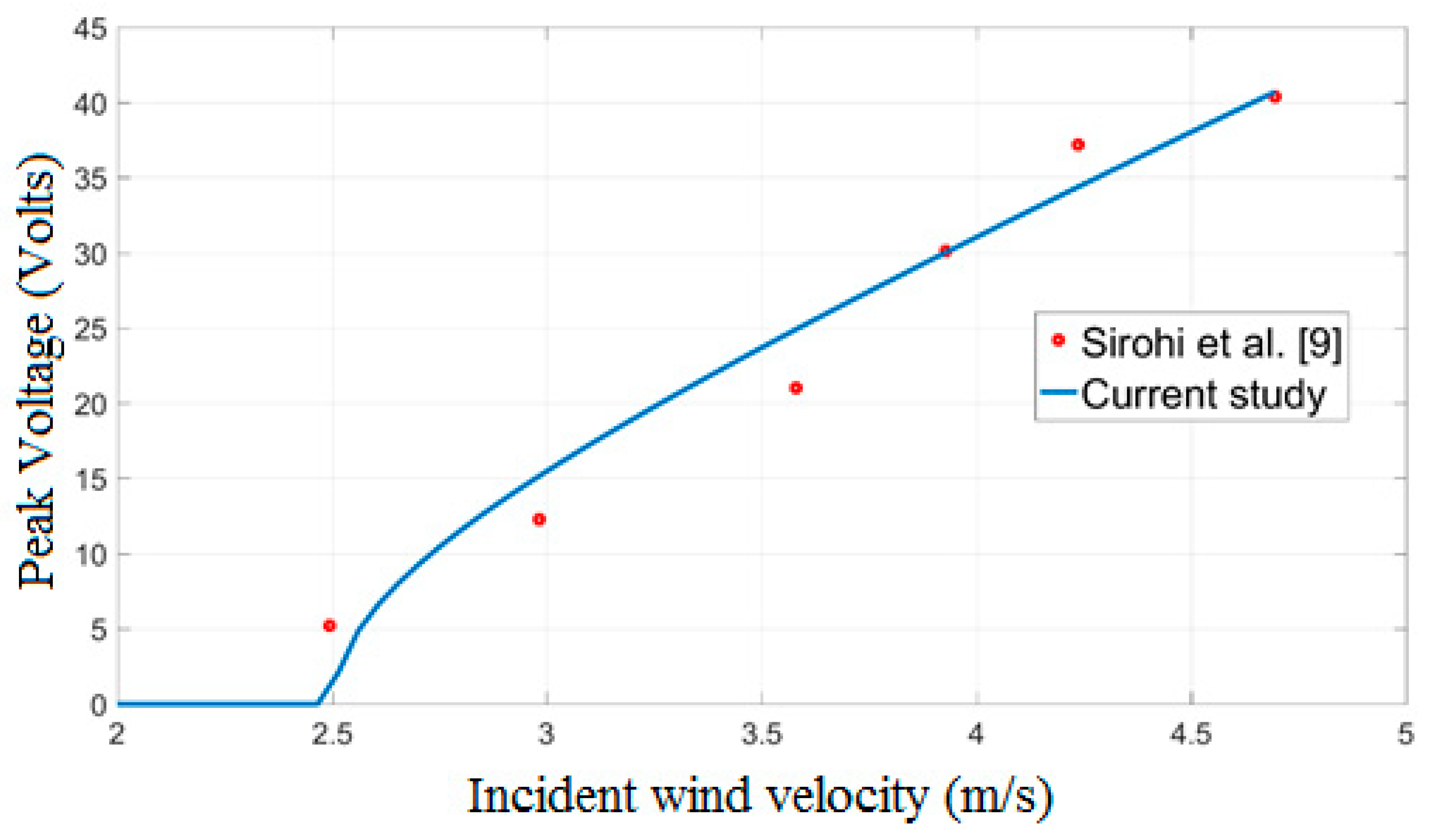
9] are
a1 = 7.2 and
a3 = −2.1757. Additionally, the fitted results are present in
Figure 5. The fitted coefficients predict the onset of galloping at 5.6 mph (2.5 m/s) for R = 0.7 MΩ, and the maximum error is less than 5 Volts.
Unfortunately, there is no published data other than References [
9,
16] for the problem of transverse galloping while the beam is normal to the wind direction and tip mass size in the direction of the beam (from clamped point to free end) is comparable to the beam length. More experiment results from Reference [
17] are presented in
Table 4 for validating the theoretical study and the numerical simulations. Those results are related to a tip mass of 23 g with length and width of 70 and 60 mm, respectively. Moreover, the range of wind velocity is 8–12 (m/s). Instead of a two-layer piezoelectric, Jamalabadi et al. [
17] used one piezoelectric sheet partially covering the cantilever. The start point of the piezoelectric sheet was not the clamped point for some manufacturing considerations, and the piezoelectric sheet was located at the position with the highest strain values.
Table 5 presents the numerical and experimental results of Jamalabadi et al. [
17]. As shown, the natural frequency of the system is evaluated at 7.33 Hz while the experimental data (first peak of frequency response) happens at 7.5 Hz (2 percent error).
It is good to note that, in some references, to remove the difference of the frequency gained by the numerical method and the measured frequency, a nonlinear torsional spring is considered at the clamped point for the effects of the incomplete clamp. In this study, the clamp point is considered a complete clamp condition. Also, the voltage to tip displacement of the system is evaluated with a good agreement (5 percent error), since the correction of Equation (47) is not necessary (if the correction of Equation (47) is applied, the relative error increases to 12 percent).
Figure 6 presents the variations of the voltage results of Reference [
17] for different values of wind velocity. Inspecting this figure, the theory used here fits the experimental results for
a1 = 2.416 and
a3 = −201.3095.
3.2. Effects of the Load Resistance and Tip Mass Length Ratio on the Harvester′s Response
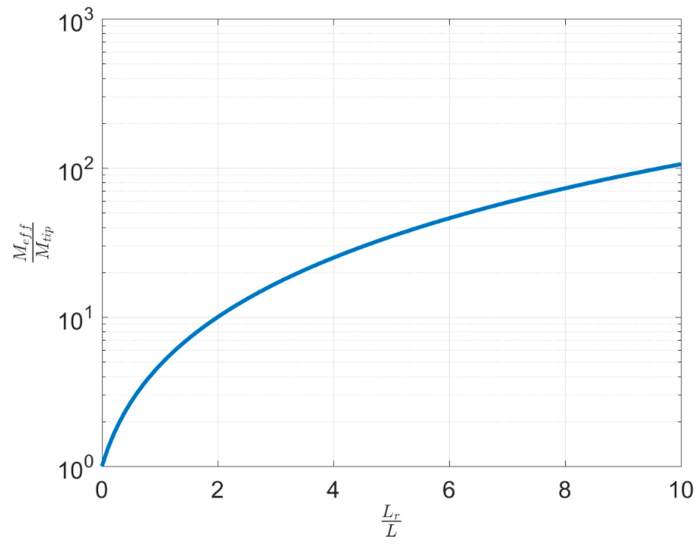
The effect of tip mass length on effective mass is plotted in
Figure 7. The curve is plotted by use of Equation (21). As shown, if the dynamic correction is not applied on the tip mass, it will lead to a higher error in the calculation of effective mass, natural frequency, etc. After the correction of
Figure 8 in calculating the effective mass, it would be ready to be used in design calculations provided for the lumped method, as presented in Reference [
7]. For example, in the case investigated in this paper, for the tip mass length to beam length ratio (
) of 2.61, the contribution of tip mass in the effective mass is 13.95 times of its static mass. It means the total mass of the system is approximately 14 times the static mass of the tip mass. If the formulation in Reference [
9] is adopted, the value is 6.1 instead. Also, it is revealed in
Figure 8 that, if the length of the rigid tip body is ten times that of the cantilever length, the effective mass should be considered in vibrational calculations and is one hundred times the mass of the tip body.
The theoretical relation between the open-circuit voltage and the tip displacement as predicted by Equation (43) is about 570.1643 volts per each meter deflection of the tip of the beam. These values will be corrected by the phase difference angle of 3.9477 degrees which leads to the correction of 568.8111 volts per meter. It means that the maximum voltage of 34 corresponds to the deflection of 6 centimeters of tip deflection. If the correction of Reference [
9] is considered, this value decreases to 46 mm, while as the measurement of deflection is not reported in Reference [
9], it could not be compared with experimental data.
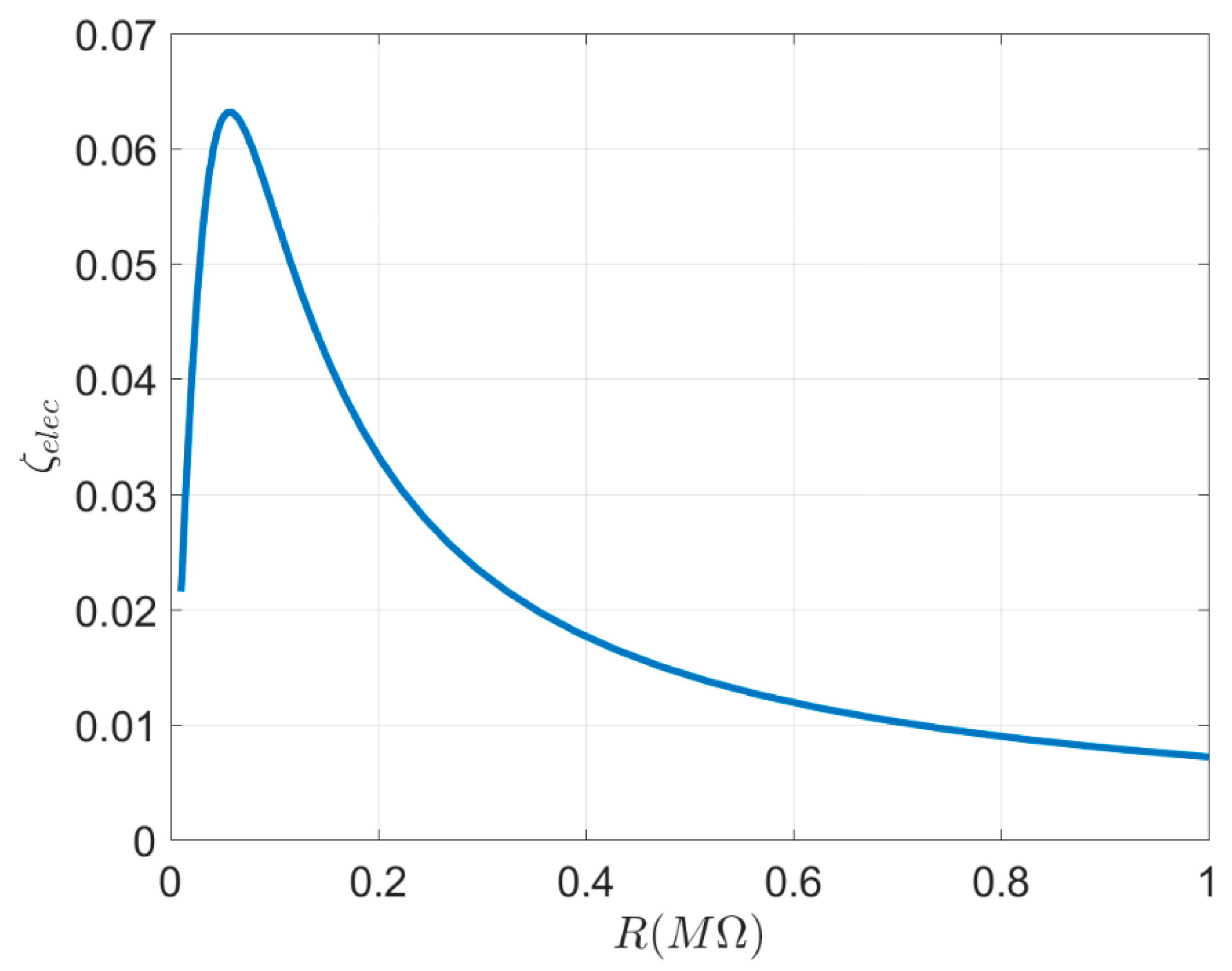
The added damping ratio by applying the electrical impedance is shown in
Figure 9. The effective damping ratio as a function of load resistance is as follows:
Figure 9 presents the equivalent damping ratio of the electrical load impedance as a function of load impedance. As shown, the minimum added damping ratio to the system at a load resistance of 0.7 MΩ is 0.01. The artificial value of 0.003 for total damping ratio at that point could not be considered. As one can observe from Equation (39), the damping coefficient should have a maximum value at a specific configuration:
At this value of resistance, the phase difference of voltage and displacement would be π/4 and the electrical damping is maximized.
Figure 9 presents the peak value when the value (R = 57 kΩ) is less than the initial range used in the experiment of Reference [
8].
To compare the power harvested in Reference [
13] with the current study, the electrical damping is defined as follows:
where
C is defined as the electrical damping resulting from the electromechanical coupling by Tan and Yan under Equation (5) in Reference [
13],
θp (here is
) is adopted by comparing their Equation (1) with Equation (48), and
. By observation in Equation (56), it is clear that, if the electrical damping ratio defined in Equation (56) is multiplied by angular velocity, the electrical damping defined in Equation (58) is obtained (
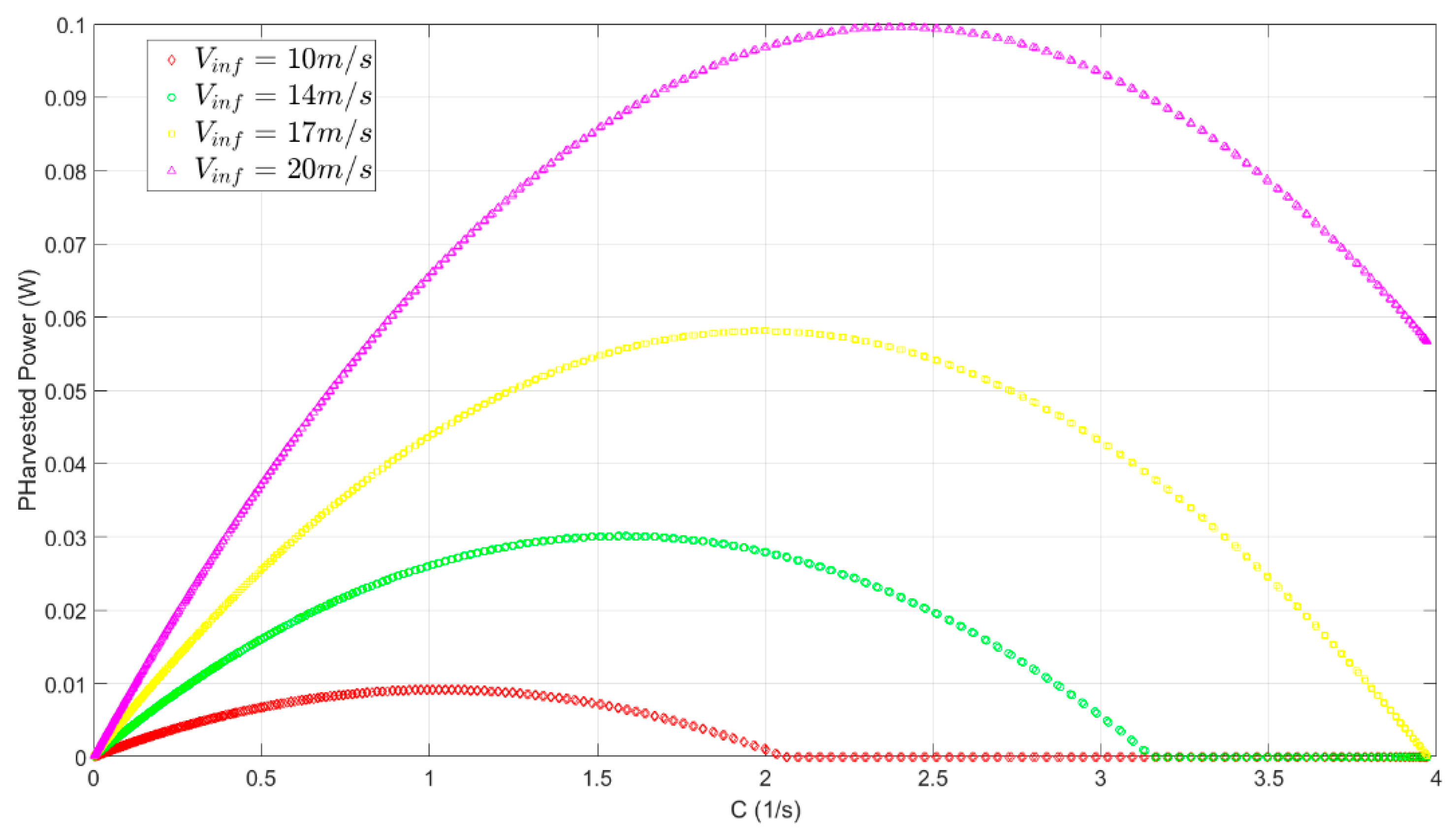
C = 2ωζe). If harvested power is considered during a period of motion
and rearranged by the definition of Equation (58), harvested power is
As seen from the above equation, Equation (58) does not presents an explicit expression of harvested power as a function of
C because, in Equation (58),
R is still a function of
C (See Equation (58).). The effects of electrical damping on the harvested power are presented in
Figure 10. For the configuration defined in
Table 1, the maximum value of
C is 3.9722.
Figure 8 reveals that even such odd wind velocities can be accessible for steady power harvesting; the amount of harvested power could not exceed 100 milliwatts. The resultant harvested power of the current case with that of References [
13,
14] based on the coefficient of
Table 2 could be compared in
Figure 10.
In the current study, the analytical solution is compared with some previous cases and it is expected that the model is useful for low-amplitude energy harvesting which is in the range of linear elastic material strain. As shown, the experimental results demonstrate that the values in
Table 2 are not valuable in the calculation of harvested power for the low-amplitude galloping regime. The a
1 value found in this study is considerably higher than the a
1 value presented in
Table 2. This estimates the onset of galloping velocity much lower than that in the experimental results (See Equation (42)). Also, the a
3 coefficient is 1 order to 2 orders of magnitude higher than the a
3 presented in
Table 2. Even the difference in estimation of onset of galloping velocity ignores the 1–2 order of magnitude difference in a
3 and could cause a one order of magnitude difference in final deflection (See Equation (39).) and voltage (See Equation (38).) and two orders of magnitude difference in power results (See Equation (44), and compare Figure 10 with Figure 4 of Reference [
17]). The difference between fitted coefficient for Reference [
9] (Re ≈ 10
4) and that of Reference [
17] (Re ≈ 10
5) could be attributed to the various characteristic lengths and ranges of velocity which lead to various Reynolds numbers. While the Reynolds number for Reference [
9] is about 11,400 the Reynolds number for Reference [
17] is about 67,260. It shows that, to globalize the results of the aerodynamic coefficient to the problem of beam galloping perpendicular to the wind direction, more experiments are needed.


