Subspace Reduction for Stochastic Planar Elasticity

Abstract

Stochastic eigenvalue problems are nonlinear and multiparametric. They require their own solution methods and remain one of the challenge problems in computational mechanics. For the simplest possible reference problems, the key is to have a cluster of at the low end of the spectrum. If the inputs, domain or material, are perturbed, the cluster breaks and tracing of the eigenpairs become difficult due to possible crossing of the modes. In this paper we have shown that the eigenvalue crossing can occur within clusters not only by perturbations of the domain, but also of material parameters. What is new is that in this setting, the crossing can be controlled; that is, the effect of the perturbations can actually be predicted. Moreover, the basis of the subspace is shown to be a well-defined concept and can be used for instance in low-rank approximation of solutions of problems with static loading. In our industrial model problem, the reduction in solution times is significant.

1. Introduction

Vibration problems with uncertain data are common in engineering. From the point of view of applied mathematics, development of the solution methods for this class of problems remains one of the final frontiers. Various approaches for stochastic eigenproblems have been proposed in relation to so-called stochastic finite element methods (SFEM). As always with probabilistic problems, the baseline solution technique is the Monte Carlo method [1]. The justification for the new approaches is that they have provably faster convergence rates than the Monte Carlo. Broadly speaking, the methods can be divided into invasive (e.g., Galerkin methods [2,3]) or non-invasive ones (for instance, stochastic collocation [4]). Our discussion here applies to the problem of resolving the smallest eigenmode when the design configuration has uncertainties.

Some applications of uncertainty quantification to investigate the static and dynamical responses of beam, plates, and shells with random parameters are found in the literature. We mention two papers that also have considered Young’s modulus as a random quantity. Bahmyari et al. [5] provided a bending analysis of thick plates with elastically restrained edges and resting on Pasternark elastic foundation, where the plate’s Young’s modulus and stiffness of the boundary conditions and elastic foundation were assumed as random variables. The free vibrations of orthotropic plates with uncertainties in the Young’s modulus were investigated by Ernst et al. [6] who obtained good correlation between experimental and numerical results.

In computational vibration or dynamic analysis of deterministic problems, the methods used in static loading problems can be applied directly. For the stochastic problem, this useful connection between dynamic and static problems is broken. The uncertainties, such as fluctuations in the material parameters, are random variables represented using series with random coefficients that are the stochastic parameters. One immediate consequence is that normalization of the eigenmodes has to be valid over the whole parameter space. This global normalization constraint in fact makes the problem nonlinear as opposed to its deterministic counterpart. Moreover, current mathematical analysis (see, e.g., [4,7]) is based on second-order model problems where it is guaranteed that the smallest mode is well-isolated and hence the question of subspace convergence is still not resolved and is the subject of current research.

Our interest is in static analysis with low-rank approximation which is enabled by accurately resolving the correct eigenspaces. Identification of subdomains with high variance in stress components, say, could be useful in sensor placement design for online failure detection (For an exhaustive recent review, see [8]).

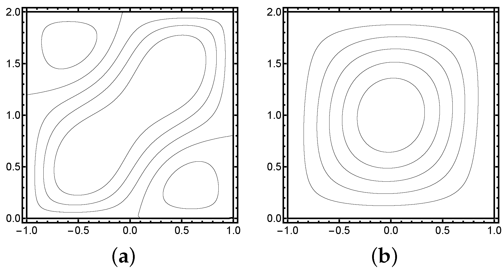
What distinguishes the vibration problems in mechanics from the classical model problem in analysis is that the smallest mode can in fact be of higher multiplicity. This follows directly from symmetries. For planar elasticity, our chosen setting, free vibration on a symmetric domain, leads to double eigenvalues or clusters of dimension two. This makes it the ideal model problem for stochastic eigenvalue problems.

Let us consider free vibration on a square plate (see Figure 1). The smallest eigenvalue is a double one, and two modes have simply interchanged the respective profiles on the vector fields u and v. However, if the domain is perturbed, for instance, extended in either one of the coordinate directions, the cluster breaks apart and either one of the modes becomes the true smallest one. If this phenomenon is described in terms of uncertain domains, we see that the eigenpairs $({\kappa }_1,{\mathbf{u}}_1)$ and $({\kappa }_2,{\mathbf{u}}_2)$, say, depend on the random variable $\omega$, and crucially, if we trace the smallest eigenvalue ${\kappa }_{min}=min\{{\kappa }_1(\omega ),{\kappa }_2(\omega )\}$, the corresponding eigenmode may change, that is, the eigenmode is not consistent over the whole parameter space and we say that the eigenvalues cross. Hence, to emphasize this nontrivial dependence of the eigenmodes on $\omega$, we call ${\kappa }_{min}={\kappa }_{min}(\omega )$ the effective smallest eigenvalue over the parameter space. We note that considering the corresponding eigenmode is problematic in the sense that such an eigenmode would change discontinuously in the proximity of the crossing.

This paper has two objectives: First, we illustrate that the question of the effective smallest eigenvalue can arise within planar elasticity, and second, despite the inherent ambiguity of the eigenvalues within a subspace, a basis of the subspace can be used in low-rank approximation of standard source problems. In the computational experiment, we demonstrate the efficacy of the subspace construction in terms of computational complexity in a problem with non-trivial geometry. Our model problem, an idealized 2D crankshaft section with random Young’s modulus, was initially proposed as an initial step in a metal fatigue problem related to ship engines.

The rest of the paper is structured as follows: First we cover preliminaries in Section 2, including the Navier’s equations of elasticity, their stochastic formulation, and the collocation method used here. Subspace construction is given in Section 3. Eigenvalue crossing is discussed in Section 4. Computational study of a 2D crankshaft model highlights the low-rank solution method in Section 5. Finally, conclusions are drawn in the final section.

2. Preliminaries

In this section, we give a brief overview of the (stochastic) model of planar elasticity and the collocation method used in the solution of stochastic problems.

2.1. Navier’s Equations of Elasticity

We use the Navier’s equations of elasticity to model the system of interest. Let D be a domain representing a deformable medium subject to a body force $\mathbf{f}$ and a surface traction $\mathbf{g}$. The 2D model problem is then to find the displacement field $\mathbf{u}=(u_1,u_2)$, and the symmetric stress tensor $\sigma ={({\sigma }_{ij})}_{i,j=1}^2$, such that

$$\begin{array}{ccc}\hfill \sigma & =\lambda div(\mathbf{u})\mathit{I}+2\mu ϵ(\mathbf{u}),\hfill & \hfill \mathrm{in}D\\ \hfill -div(\sigma )& =\mathbf{f},\hfill & \hfill \mathrm{in}D\\ \hfill \mathbf{u}& =\mathbf{0},\hfill & \hfill \mathrm{on}\partial D_D\\ \hfill \sigma ·\mathbf{n}& =\mathbf{g},\hfill & \hfill \mathrm{on}\partial D_N\end{array}$$

(1)

where $\partial D=\partial D_D\cup \partial D_N$ is a partitioned boundary of D. The Lamé constants are

$$\lambda =\frac{E\nu }{(1+\nu )(1-2\nu )},\mu =\frac{E}{2(1+\nu )},$$

(2)

with E and $\nu$ being Young’s modulus and Poisson’s ratio, respectively. Further, $\mathit{I}$ is the identity tensor, $\mathbf{n}$ denotes the outward unit normal to $\partial D_N$, and the strain tensor is

$$ϵ(\mathbf{u})=\frac{1}{2}(\nabla \mathbf{u}+\nabla {\mathbf{u}}^T).$$

(3)

The vector-valued tensor divergence is

$$div(\sigma )={\left(\sum _{j=1}^2\frac{\partial {\sigma }_{ij}}{\partial x_j}\right)}_{i=1}^2.$$

(4)

This formulation assumes a constitutive relation corresponding to linear isotropic elasticity with stresses and strains related by Hooke’s generalized law

$${\sigma }_v=\left[\begin{array}{c}{\sigma }_{11}\\ {\sigma }_{22}\\ {\sigma }_{12}\end{array}\right]=\mathbf{D}(\lambda ,\mu )\left[\begin{array}{c}{ϵ}_{11}\\ {ϵ}_{22}\\ {ϵ}_{12}\end{array}\right]=\mathbf{D}(\lambda ,\mu ){ϵ}_v.$$

(5)

2.1.1. Weak Formulation

Let us introduce a function space $V_D=\{v:v\in H^1(D),v{|}_{\partial D_D}=0\}$, and state: Find $\mathbf{u}\in V_D\times V_D$ such that

$$a(\mathbf{u},\mathbf{v})=L(\mathbf{u}),\forall \mathbf{v}\in V_D\times V_D,$$

(6)

where the bilinear form

$$a(\mathbf{u},\mathbf{v})={\int }_D\sigma (\mathbf{u}):ϵ(\mathbf{v})d\mathbf{x}$$

(7)

is the integrated tensor contraction

$$\sigma :ϵ=\sum _{i,j=1}^2{\sigma }_{ij}{ϵ}_{ij},$$

(8)

and $L(·)$ denotes the linear functional

$$L(\mathbf{v})={(\mathbf{f},\mathbf{v})}_D+{(\mathbf{g},\mathbf{v})}_{\partial D_N}={\int }_D\mathbf{f}·\mathbf{v}d\mathbf{x}+{\int }_{\partial D_N}\mathbf{g}·\mathbf{v}d\mathbf{s}.$$

(9)

As usual, we define the kinematic relation

$${ϵ}_v(\mathbf{u})=\left[\begin{array}{cc}\frac{\partial }{\partial x_1}& 0\\ 0& \frac{\partial }{\partial x_2}\\ \frac{\partial }{\partial x_2}& \frac{\partial }{\partial x_1}\end{array}\right]\left[\begin{array}{c}{u}_1\\ u_2\end{array}\right]$$

(10)

and specify the constitutive matrix

$$\mathbf{D}(\lambda ,\mu )=\left[\begin{array}{ccc}\lambda +2\mu & \lambda & 0\\ \lambda & \lambda +2\mu & 0\\ 0& 0& \mu \end{array}\right]$$

(11)

for the purpose of rewriting the bilinear form as

$$a(\mathbf{u},\mathbf{v})={\int }_D{ϵ}_v{(\mathbf{u})}^T\mathbf{D}(\lambda ,\mu ){ϵ}_v(\mathbf{v})d\mathbf{x}.$$

(12)

2.1.2. Stochastic Formulation

We introduce a stochastic extension of Navier’s equations of elasticity, which we will consider for the remainder of this paper. Letting $(\mathsf{\Omega },\Gamma ,P)$ denote a probability space, where $\mathsf{\Omega }$ is a space of outcomes, $\Gamma \subset 2^{\mathsf{\Omega }}$ a sigma-algebra of events, and $P:\mathsf{\Omega }\to [0,1]$ a probability measure on $\mathsf{\Omega }$, respectively, we model the uncertainties in the domain and material parameters of the physical problem (1) by assuming that there exists an explicit dependence of these quantities on the stochastic variable $\omega \in \mathsf{\Omega }$ via a priori known mappings $\omega \mapsto D^{\omega }$, $\omega \mapsto E^{\omega }$, $\omega \mapsto {\mathbf{f}}^{\omega }$, and $\omega \mapsto {\mathbf{g}}^{\omega }$.

The stochastic problem can then be stated as: find the displacement field ${\mathbf{u}}^{\omega }:D^{\omega }\to {\mathbb{R}}^2$ and stress tensor ${\sigma }^{\omega }:D^{\omega }\to {\mathbb{R}}^{2\times 2}$ such that

$$\begin{array}{ccc}\hfill {\sigma }^{\omega }& ={\lambda }^{\omega }div({\mathbf{u}}^{\omega })\mathit{I}+2{\mu }^{\omega }ϵ({\mathbf{u}}^{\omega }),\hfill & \hfill \mathrm{in}{D}^{\omega }\\ \hfill -div({\sigma }^{\omega })& ={\mathbf{f}}^{\omega },\hfill & \hfill \mathrm{in}{D}^{\omega }\\ \hfill {\mathbf{u}}^{\omega }& =\mathbf{0},\hfill & \hfill \mathrm{on}\partial D_{D^{\omega }}\\ \hfill {\sigma }^{\omega }·\mathbf{n}& ={\mathbf{g}}^{\omega },\hfill & \hfill \mathrm{on}\partial D_N^{\omega }\end{array}$$

(13)

for P-almost every $\omega \in \mathsf{\Omega }$. Here the stochastic dependence $\omega \mapsto E^{\omega }$ is propagated also into the Lamé constants ${\lambda }^{\omega }$ and ${\mu }^{\omega }$ via the Equation (2).

Analogously to the deterministic case, the stochastic system (13) can also be expressed in weak form. Let us define stochastic extensions for the forms (7) and (9) by setting

$$a(\omega ;\mathbf{u},\mathbf{v})={\int }_{D^{\omega }}{\sigma }^{\omega }(\mathbf{u}):ϵ(\mathbf{v})d\mathbf{x}$$

(14)

and

$$L(\omega ;\mathbf{v})={({\mathbf{f}}^{\omega },\mathbf{v})}_{D^{\omega }}+{({\mathbf{g}}^{\omega },\mathbf{v})}_{\partial D_N^{\omega }}.$$

(15)

The weak form of the stochastic problem then reads: find ${\mathbf{u}}^{\omega }\in V_{D^{\omega }}\times V_{D^{\omega }}$ such that

$$a(\omega ;{\mathbf{u}}^{\omega },\mathbf{v})=L(\omega ;{\mathbf{u}}^{\omega })\forall \mathbf{v}\in V_{D^{\omega }}\times V_{D^{\omega }}$$

(16)

for P-almost every $\omega \in \mathsf{\Omega }$.

The spatial and stochastic dimensions of the system are decoupled: each individual realization of $\omega \in \mathsf{\Omega }$ fixes the measurement configuration—the geometry $D^{\omega }$ and the inputs $E^{\omega }$, ${\mathbf{f}}^{\omega }$ and ${\mathbf{g}}^{\omega }$ – and corresponds to one instance of the deterministic problem (1), which can be solved numerically using FEM. The stochastic problem can be solved through stochastic collocation, which is tantamount to solving an ensemble of deterministic problems corresponding to a list of collocation nodes $({\omega }_1,\dots ,{\omega }_N)$ in $\mathsf{\Omega }$.

The solution of the stochastic problem can be used for determining the response statistics of any quantity of interest defined for the solution pair $({\mathbf{u}}^{\omega },{\sigma }^{\omega })$ with respect to any assumed uncertainties in the initial measurement setting. We consider the expectations and variances of the norms of the stresses of the stochastic elasticity problem given by

$$\begin{array}{cc}\hfill \mathbb{E}[\rho (\sigma )]& ={\int }_{\mathsf{\Omega }}\rho ({\sigma }^{\omega })\mathrm{d}P(\omega )\hfill \end{array}$$

(17)

$$\begin{array}{cc}\hfill \mathrm{Var}[\rho (\sigma )]& =\mathbb{E}\left[\rho {(\sigma )}^2\right]-\mathbb{E}{\left[\rho (\sigma )\right]}^2,\hfill \end{array}$$

(18)

where $\rho$ stands in for the spatial $L^2$ and $H^1$ norms, respectively.

2.1.3. Stochastic Eigenproblem

The stochastic eigenproblem corresponding to the Navier’s equations given in (13) is obtained by replacing the body force ${\mathbf{f}}^{\omega }$ with a multiple of the displacement field ${\mathbf{u}}^{\omega }$ itself. The problem then reads: find the eigenvalue ${\kappa }^{\omega }\in \mathbb{R}$, the eigenvector ${\mathbf{u}}^{\omega }:D^{\omega }\to {\mathbb{R}}^2$, and the stress tensor ${\sigma }^{\omega }:D^{\omega }\to {\mathbb{R}}^{2\times 2}$ such that

$$\begin{array}{ccc}\hfill {\sigma }^{\omega }& ={\lambda }^{\omega }div({\mathbf{u}}^{\omega })\mathbf{I}+2{\mu }^{\omega }ϵ({\mathbf{u}}^{\omega }),\hfill & \hfill \mathrm{in}{D}^{\omega }\\ \hfill -div({\sigma }^{\omega })& ={\kappa }^{\omega }{\mathbf{u}}^{\omega },\hfill & \hfill \mathrm{in}{D}^{\omega }\\ \hfill {\mathbf{u}}^{\omega }& =\mathbf{0},\hfill & \hfill \mathrm{on}\partial D_{D^{\omega }}\\ \hfill {\sigma }^{\omega }·\mathbf{n}& ={\mathbf{g}}^{\omega },\hfill & \hfill \mathrm{on}\partial D_N^{\omega }\end{array}$$

(19)

for P-almost every $\omega \in \mathsf{\Omega }$. To make the eigenmodes physically meaningful, we also impose that ${\mathbf{u}}^{\omega }$ is normalized in $L^2(D^{\omega })$ for P-almost every $\omega \in \mathsf{\Omega }$.

The weak form of the stochastic eigenproblem is: find the eigenvalue ${\kappa }^{\omega }\in \mathbb{R}$ and eigenvector ${\mathbf{u}}^{\omega }\in V_{D^{\omega }}\times V_{D^{\omega }}$ such that

$$a(\omega ;{\mathbf{u}}^{\omega },\mathbf{v})={\kappa }^{\omega }{({\mathbf{u}}^{\omega },\mathbf{v})}_{D^{\omega }}\forall \mathbf{v}\in V_{D^{\omega }}\times V_{D^{\omega }}$$

(20)

for P-almost every $\omega \in \mathsf{\Omega }$. For each fixed $\omega \in \mathsf{\Omega }$, the eigenproblem (19) admits a countable number of eigenvalues that can be enumerated in increasing magnitude (counting multiplicities)

$${\kappa }_1^{\omega }\le {\kappa }_2^{\omega }\le {\kappa }_3^{\omega }\le \dots$$

(21)

and corresponding eigenvectors ${\{{\mathbf{u}}_i^{\omega }\}}_{i=1}^{\infty }$ that form a basis of $L^2(D^{\omega })$. However, due to the eigenvalue crossings mentioned in the introduction, this enumeration of the eigenmodes becomes problematic when the eigenmodes are viewed as functions of $\omega$. Instead, in Section 3, we consider resolving a basis for the subspace corresponding to a finite set of the eigenvalues and hence effectively avoid the question about the enumeration.

2.2. Stochastic Collocation

Standard stochastic finite element methods, in particular the stochastic collocation method considered here, assume that the dependence on the abstract variable $\omega$ can be parametrized using a countable set of mutually independent random variables. Such a parametrization can sometimes be known a priori or it can be estimated statistically. For the material parameters such as the Young’s modulus $E^{\omega }$, a representation of the form

$$\begin{array}{c}\hfill E^{\omega }(\mathbf{x})=E_0(\mathbf{x})+\sum _{m=1}^{\infty }{f}_m(\mathbf{x})Y_m(\omega ),\end{array}$$

(22)

is typically assumed. Here ${\{f_m\}}_{m\ge 0}$ are spatial stochastic fluctuations decaying in $L^{\infty }$-norm, as $m\to \infty$ and ${\{Y_m\}}_{m\ge 1}$ is a family of random variables assumed to be i.i.d. The series (22) can be viewed as the Karhunen–Loevé expansion of the random underlying random field, in which case the functions $f_m(\mathbf{x})$ are the eigenfunctions of some covariance function $C(x_1,x_2)$. In some simple geometric settings, these eigenfunctions are known explicitly, but they can also be resolved numerically as eigenvectors of the sampled covariance matrix; see, e.g., (Chapter 8) in [1,9] and [10]. For numerical computations, the series is truncated after M terms.

In the following paragraphs, we consider an anisotropic Smolyak-type collocation operator defined with respect to a finite multi-index set (see, e.g., [4,11,12,13]). In principle, a simpler formulation would also suffice for the purpose of our numerical experiments. However, we wish to keep the general form of the operator here, since it allows for efficient computation even in high-dimensional parameter spaces.

For the sake of accuracy, it is standard practice to choose the collocation points to be the abscissae of orthogonal polynomials; see [14]. Here we formulate the collocation method using Legendre polynomials which are the optimal choice when the input random variables are uniform. For example, in the case of Gaussian random variables, one should use Hermite polynomials instead, but otherwise the collocation method remains the same.

Let $L_p$ be the univariate Legendre polynomial of degree p. Denote by ${\{{\chi }_k^{(p)}\}}_{k=0}^p$ the zeros of $L_{p+1}$ and by ${\{w_k^{(p)}\}}_{k=0}^p$ the associated Gauss–Legendre quadrature weights. We define the one-dimensional Lagrange interpolation operators ${\mathcal{I}}_p^{(m)}$ via

$$\left({\mathcal{I}}_p^{(m)}v\right)(Y_m)=\sum _{k=0}^{p}v\left({\chi }_k^{(p)}\right){\ell }_k^{(p)}(Y_m),$$

(23)

where ${\{{\ell }_k^{(p)}\}}_{k=0}^p$ are the related Lagrange basis polynomials of degree p. Observe that

$${\int }_{-1}^1\left({\mathcal{I}}_p^{(m)}v\right)(Y_m)\frac{d{Y}_m}{2}=\sum _{k=0}^{p}v\left({\chi }_k^{(p)}\right)w_k^{(p)}.$$

(24)

Now let $\mathcal{A}\subset {\mathbb{N}}_0^M$ be a finite set of multi-indices. For $\alpha ,\beta \in \mathcal{A}$, we write $\alpha \le \beta$ if ${\alpha }_m\le {\beta }_m$ for all $m=1,\dots ,M$. We assume that $\mathcal{A}$ is monotone in the following sense:

$$\exists \alpha \in \mathcal{A}\mathrm{such}\mathrm{that}\beta \le \alpha \Rightarrow \beta \in \mathcal{A}.$$

(25)

The sparse collocation operator is defined as

$${\mathcal{I}}_{\mathcal{A}}:=\sum _{\alpha \in \mathcal{A}}\underset{m=1}{\overset{M}{⨂}}\left({\mathcal{I}}_{{\alpha }_m}^{(m)}-{\mathcal{I}}_{{\alpha }_m-1}^{(m)}\right),$$

(26)

where ${\mathcal{I}}_{-1}^{(m)}:=0.$ This may be rewritten in a computationally more convenient form

$${\mathcal{I}}_{\mathcal{A}}=\sum _{\alpha \in \mathcal{A}}\sum _{\beta \in {\mathcal{G}}_{\alpha }}{(-1)}^{{\left|\right|\alpha -\beta ||}_1}\underset{m=1}{\overset{M}{⨂}}{\mathcal{I}}_{{\beta }_m}^{(m)},$$

(27)

where ${\mathcal{G}}_{\alpha }:=\{\beta \in {\mathbb{N}}_0^M|\alpha -1\le \beta \le \alpha \}$. The collocation points are of the form

$$\begin{array}{c}\hfill {\chi }_{\gamma }^{(\alpha )}=\left({\chi }_{{\gamma }_1}^{({\alpha }_1)},\dots ,{\chi }_{{\gamma }_M}^{({\alpha }_M)}\right)\in \Gamma \end{array}$$

(28)

for some $\gamma \in {\mathbb{N}}_0^M$ such that $\gamma \le \alpha \in \mathcal{A}$. Similarly, we define the tensorized quadrature weights $w_{\gamma }^{(\alpha )}=w_{{\gamma }_1}^{({\alpha }_1)}\cdots w_{{\gamma }_M}^{({\alpha }_M)}$. Statistics, such as the expected value and variance, for the collocated solution may now be computed by applying the quadrature rule

$$\mathbb{E}\left[\underset{m=1}{\overset{M}{⨂}}{\mathcal{I}}_{{\alpha }_m}^{(m)}v\right]=\sum _{\gamma \le \alpha }v\left({\chi }_{\gamma }^{(\alpha )}\right)w_{\gamma }^{(\alpha )}$$

(29)

on the terms in Equation (27).

The accuracy of the collocated approximation is ultimately determined by the smoothness of the solution as well as the choice of the multi-index set $\mathcal{A}\subset {\mathbb{N}}_0^M$. We refer to [4,12] for a detailed analysis. In this paper, we use tensor product grids defined by

$$\mathcal{A}=\{\alpha \in {\mathbb{N}}_0^M|{\alpha }_m\le p,m=1,\dots ,M\},p\in {\mathbb{N}}_0$$

(30)

as well as multi-index sets of the form

$$\mathcal{A}=\left\{\alpha \in {\mathbb{N}}_0^M|\prod _{m=1}^M{\eta }_m^{{\alpha }_m}>ϵ\right\},ϵ>0,$$

(31)

where ${\{{\eta }_m\}}_{m=1}^M$ is a (typically decreasing) sequence of numbers in the interval $(0,1)$. Multi-index sets of the latter form have previously been employed in, for instance, [15,16].

3. Subspace Reduction

Given a finite set of indices $J=\{j_1,\dots j_S\}\subset \mathbb{N}$, let us denote by ${\mathbf{U}}_J^{\omega }=\mathrm{span}{\{{\mathbf{u}}_j^{\omega }\}}_{j\in J}$ the subspace associated to the eigenvalues ${\{{\kappa }_j^{\omega }\}}_{j\in J}$ of the problem (19). To avoid problems with possible eigenvalue crossings, we define a canonical basis for the subspace ${\mathbf{U}}_J^{\omega }$ by setting

$${\widehat{\mathbf{u}}}_i^{\omega }=\sum _{j\in J}{\mathbf{u}}_j^{\omega }{({\mathbf{v}}_i,{\mathbf{u}}_j^{\omega })}_{D^{\omega }},i=1,\dots ,S,$$

(32)

i.e., each canonical basis vector ${\widehat{\mathbf{u}}}_i^{\omega }$ is just the projection of some constant reference vector ${\mathbf{v}}_i$ onto the subspace ${\mathbf{U}}_J^{\omega }$. The reference vectors ${\{{\mathbf{v}}_i\}}_{i=1}^S$ can for instance be chosen as the eigenvectors ${\{{\mathbf{u}}_i^{\omega }\}}_{i\in J}$ evaluated at some fixed value of $\omega \in \mathsf{\Omega }$. Note that as long as the Gram matrix ${\mathbf{G}}^{\omega }:={\{({\mathbf{v}}_i,{\mathbf{u}}_j^{\omega })\}}_{i,j=1}^S$ is non-singular, the vectors ${\{{\widehat{\mathbf{u}}}_i^{\omega }\}}_{i=1}^S$ in fact form a basis of ${\mathbf{U}}_J^{\omega }$. Moreover, each ${\widehat{\mathbf{u}}}_i^{\omega }$ is now independent of the enumeration of the eigenmodes $({\kappa }_j^{\omega },{\mathbf{u}}_j^{\omega })$. In the numerical experiments of Section 5, we choose ${\{{\mathbf{v}}_i\}}_{i=1}^S$ to be the eigenvectors evaluated at $Y_m=0$ for all m in the series (22). Finally, observe that we can apply the Gram–Schmidt process to orthogonalize the basis ${\{{\widehat{\mathbf{u}}}_i^{\omega }\}}_{i=1}^S$ at each $\omega \in \mathsf{\Omega }$.

Denote by $\mathbf{A}(\omega )\in {\mathbb{R}}^{N\times N}$ and $\mathbf{M}(\omega )\in {\mathbb{R}}^{N\times N}$ the stochastic stiffness and mass matrices obtained from a finite element discretization of the Equation (20). Suppose that $\widehat{\mathbf{U}}(\omega )\in {\mathbb{R}}^{N\times S}$ is a matrix representation of the subspace ${\mathbf{U}}_J^{\omega }$, more precisely, $\widehat{\mathbf{U}}(\omega )$ has as its columns the discrete approximations of the normalized canonical basis vectors ${\{{\widehat{\mathbf{u}}}_i^{\omega }\}}_{i\in J}$. Then a low rank approximation of $\mathbf{A}(\omega )$ is obtained from

$$\widehat{\mathbf{A}}(\omega )=\mathbf{M}(\omega )\widehat{\mathbf{U}}(\omega ){\widehat{\mathbf{U}}}^{\mathrm{T}}(\omega )\mathbf{A}(\omega )\widehat{\mathbf{U}}(\omega ){\widehat{\mathbf{U}}}^{\mathrm{T}}(\omega )\mathbf{M}(\omega ),$$

(33)

where ${\widehat{\mathbf{U}}}^{\mathrm{T}}(\omega )\mathbf{A}(\omega )\widehat{\mathbf{U}}(\omega )$ is now a matrix of size $S\times S$.

Instead of the generalized eigenproblem implied by Equation (20), one may also consider the standard eigenproblem of the matrix $\mathbf{A}(\omega )$ with eigenvectors normalized in ${\mathbb{R}}^N$. If we again collect the discrete approximations of the resulting normalized canonical basis vectors into a matrix $\widehat{\mathbf{Q}}(\omega )\in {\mathbb{R}}^{N\times S}$, then an alternative low-rank approximation for $\mathbf{A}(\omega )$ is obtained simply from

$$\widehat{\mathbf{A}}(\omega )=\widehat{\mathbf{Q}}(\omega ){\widehat{\mathbf{Q}}}^{\mathrm{T}}(\omega )\mathbf{A}(\omega )\widehat{\mathbf{Q}}(\omega ){\widehat{\mathbf{Q}}}^{\mathrm{T}}(\omega ).$$

(34)

4. Eigenvalue Crossing

As we have already seen in the introduction, perturbations in the domain break the lowest mode cluster. Now we demonstrate that perturbations in the material parameters can have the same effect. The two eigenpairs of the cluster are said to cross, that is, the mode associated with the smallest eigenvalue can change within the parameter space.

In the context of our study, we model the Young’s modulus as random and represent it formally as a truncated Karhunen–Loève expansion in the spirit of (22):

$$\begin{array}{c}\hfill E^{\omega }(\mathbf{x})=E_0(\mathbf{x})+\sum _{m=1}^M{f}_m(\mathbf{x})Y_m(\omega ).\end{array}$$

(35)

Without loss of generality, we can assume that the distribution involved is uniform and after possible rescaling $Y_m\sim U(-1,1)$ for all $m=1,\dots ,M$, hence making it possible to employ the collocation scheme outlined above. We set $E_0(x)=1000$ (constant) and $f_m(x)=\frac{1}{\sqrt{{\lambda }_m}}sin(a_{1}mx+a_2)$, where $a_i$ are coefficients depending on the geometry, and ${\lambda }_m$ is a decaying sequence with a known rate of decay ${\lambda }_m\sim m^{-2\varsigma }$.

In the interest of reproducibility, as in one of the examples of [16], the functions $f_m(\mathbf{x})$ have been chosen independent of any covariance function. For examples of analytic variants in simple geometric setting, or discretized approximations over general domains, see (Chapter 8) in [1,17,18].

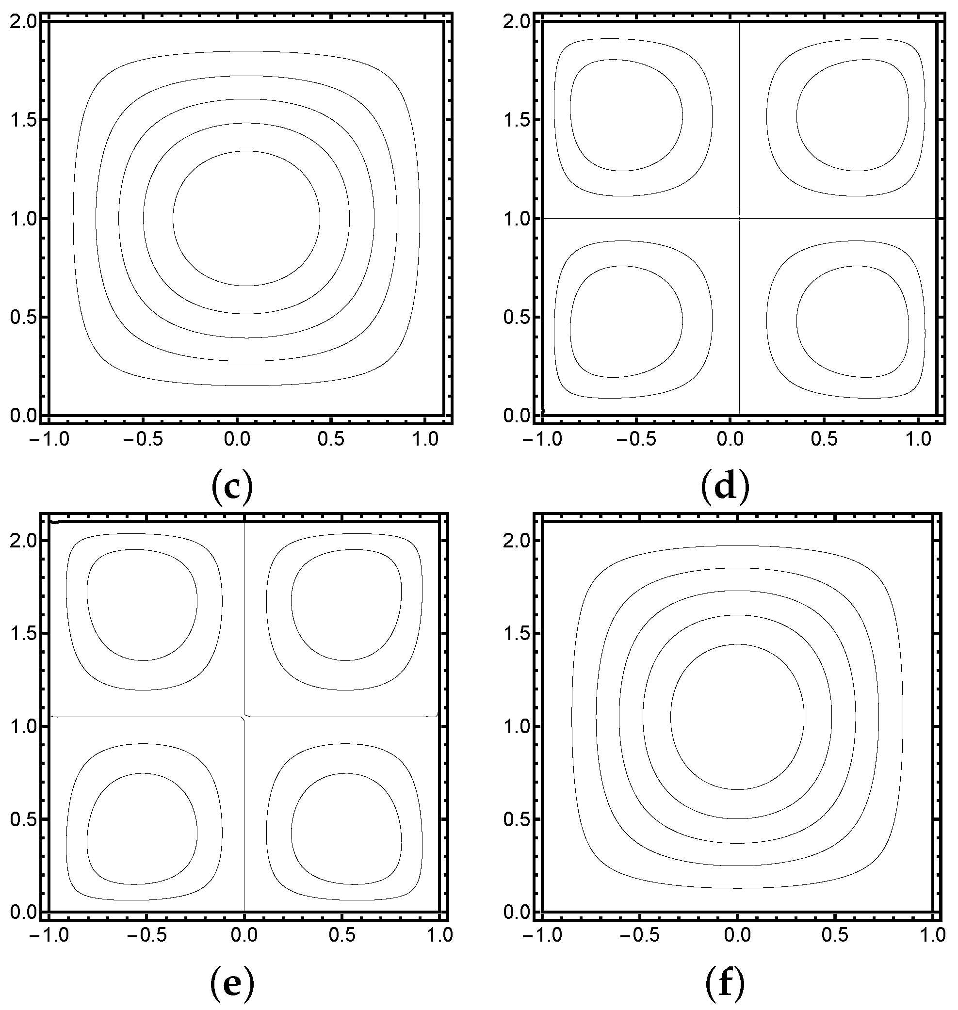
We choose $\varsigma =3$, $a_1=\pi$, $a_2=0$, and $\epsilon =1/1000$ in (31), resulting in stochastic dimension $M=21$. Crossing can then be demonstrated by taking all $Y_m=c_i$, $c_i\in [-1,1]$; that is, every $Y_m$ has the same constant value. This is shown in Figure 2. The modes cross at $Y_m=0$, since at that point the smallest mode is the cluster of dimension $=2$. Notice that the actual parameter space has dimension $=21$ in this case. In order to trace the true smallest eigenpair for all realizations, the computational complexity would be roughly equal to integration problem of the same dimension; in other words, it would be very expensive indeed.

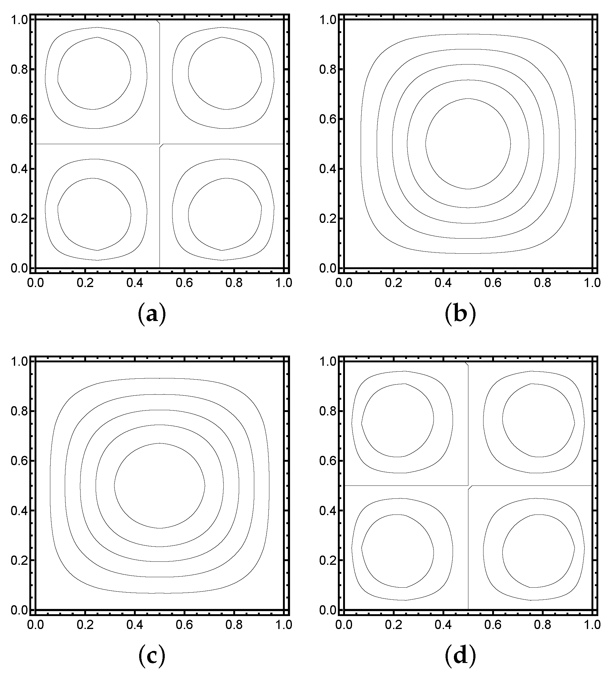
In Figure 3, it is verified that the (essentially) same two modes appear as before. The practical implication of this phenomenon is that if we sample many manufactured specimens, the variation in observed quantities of interest can actually fall within the uncertainties of the inputs rather than deficiencies in the manufacturing process.

5. Low-Rank Solution: Crankshaft Model

Even though the question of the effective eigenvalues is complicated, the subspace associated to a cluster of eigenvalues is indeed typically well defined and smooth over the whole parameter space. More precisely, it follows from classical perturbation theory that if the eigenvalues in the cluster are separated from the rest of the spectrum for all parameter values and the underlying solution operator depends analytically on the parameters, then the associated subspace also depends analytically on the parameters; see chapter VII (especially Theorem 1.7) in [19]. Therefore, such a subspace can be used in low-rank approximation. Our numerical experiment concerns a 2D configuration which is an idealized crankshaft model with a double fillet (Figure 4). This problem was originally proposed as an example of industrial uncertain domains by Prof. J. Könnö (formerly Wärtsilä, now University of Oulu) and studied in a master’s thesis [20]. In manufacturing, the errors arise from geometric imperfections and variation in material properties. In the spirit of our discussion, we study only the effects of the material parameters.

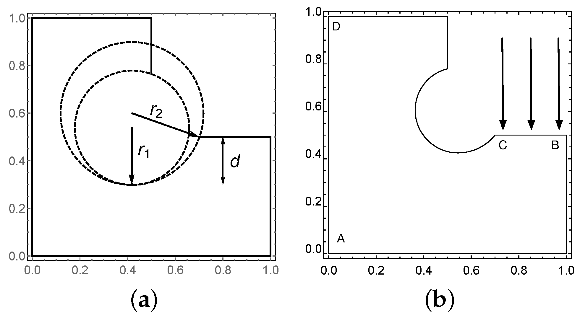
Since the material parameters (input) are uncertain or random, the quantities of interest are naturally statistical. Under fixed loading— a unit traction applied to a segment of the domain (see Figure 4)—we are interested in the expected values of the potential and stress components of the solution field components, and more importantly, the variance of these quantities and their distribution over the elastic body, here a 2D domain.

The computational domain S of the crankshaft model is formally formed by subtracting from an L-shaped domain $L={[0,1]}^2\setminus {[1/2,1]}^2$, two circles $C_1(r_1,d)=\mathbb{D}({\mathbf{c}}_1(d),r_1)$ and $C_2(r_2,d)=\mathbb{D}({\mathbf{c}}_2(d),r_2)$, with radii $r_i$, $i=1,2$, $r_2>r_1$, respectively, whose centres ${\mathbf{c}}_i$, $i=1,2$, are uniquely defined by a condition that the tangents of the two circles coincide at a point with an $x_2$-coordinate of $1/2-d$, where the “drop” d is a given parameter. Thus, every parameterized realization has the form $S(r_1,r_2,d)=L\setminus (C_1(r_1,d)\cup C_2(r_2,d))$.

In the numerical experiments, the three geometry parameters could be modeled as random variables with uniform distributions: $r_1\sim U(3/25,6/25)$, $r_2\sim U(3/20,1/4)$, and $d\sim U(1/20,1/10)$. Here we fix the values to their respective expected ones:

$$r_1=3/40,r_2=1/5,d=9/50.$$

We set the Young’s modulus as the random variable as above with decay rate $\varsigma =3$ and tolerance $\epsilon =1/100$ in (31), leading to $M=6$ and $\left|\mathcal{A}\right|=8$.

The finite element solution was carried out using second-order elements with a fine mesh resulting in each linear system with 45,772 degrees of freedom. This overrefinement was an attempt to ensure that the timing comparisons below were not affected by implementation details. The stochastic subspace has been constructed using the first 100 eigenmodes. With this choice, the average of the relative error of the low-rank approximation in the squared energy norm is less than 1%. The collocation step was carried out using a tensor product grid with 729 nodes (30).

On an iMac Pro (2017) with 18 cores and 128GB RAM, using Mathematica 12.3.1 [21], the subspace construction and a single solution set using (34) combined took $300+50=350$ s as opposed to more than 540 s for a full solution. It should be noted that the subspace construction implementation is a proof of concept, whereas the full solution used highly optimized solvers. It is clear that the potential benefits only increase with higher dimensional problems where the number of collocation points is significantly higher.

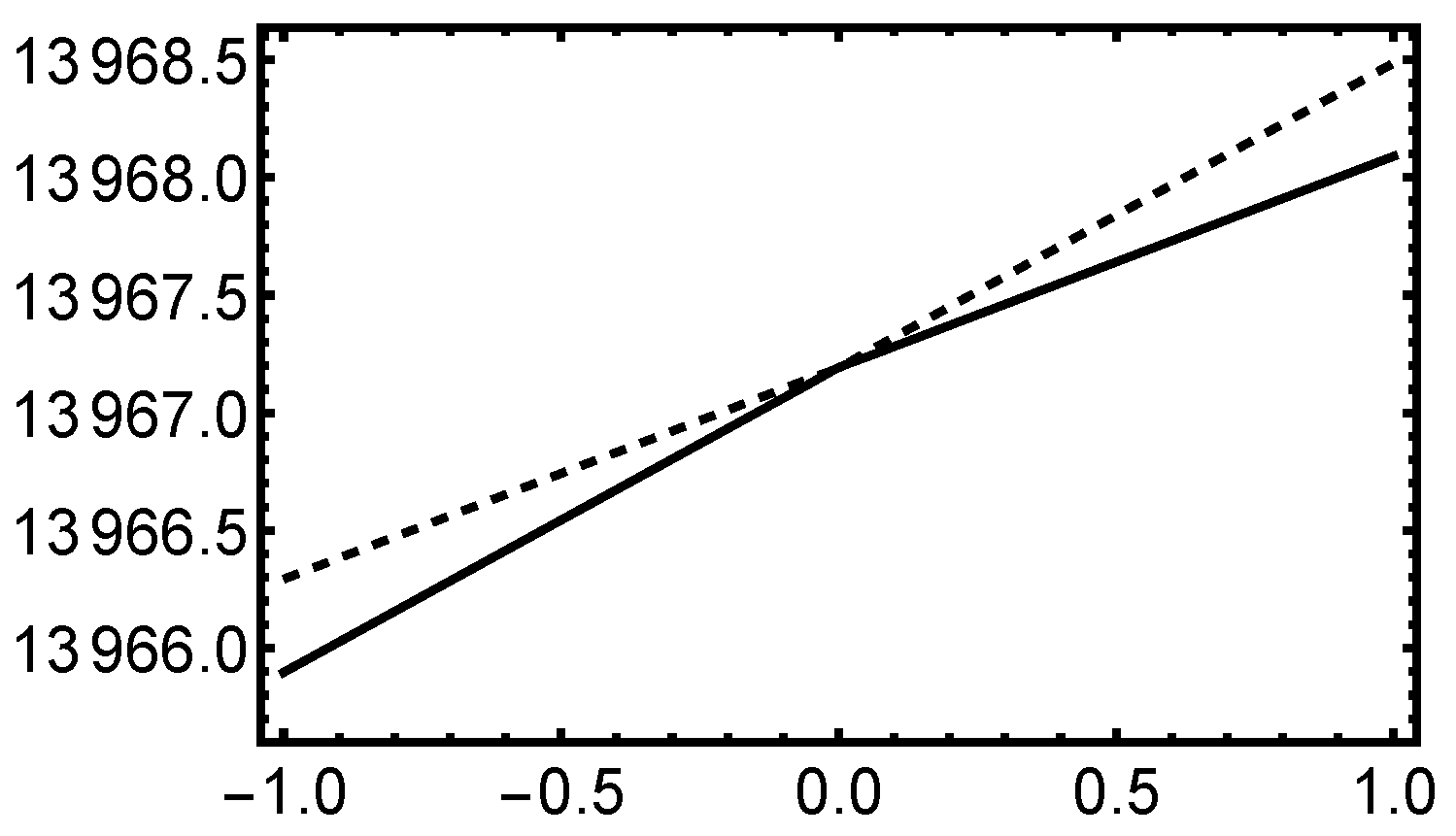
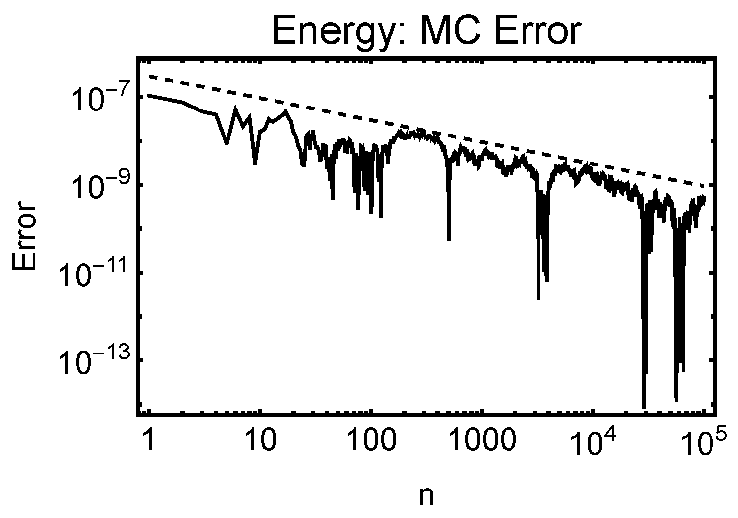
In the absense of real measurement data, any verification of the convergence of the proposed method has to be done numerically. In probabilistic setting, the Monte Carlo method always serves as the gold standard, since its expected rate of convergence in any aggregate quantity of interest is known. In Figure 5, the convergence in energy is observed to be as expected: the reference result is taken to be an overkill solution with a combination of a strongly refined mesh and high-order collocation rule.

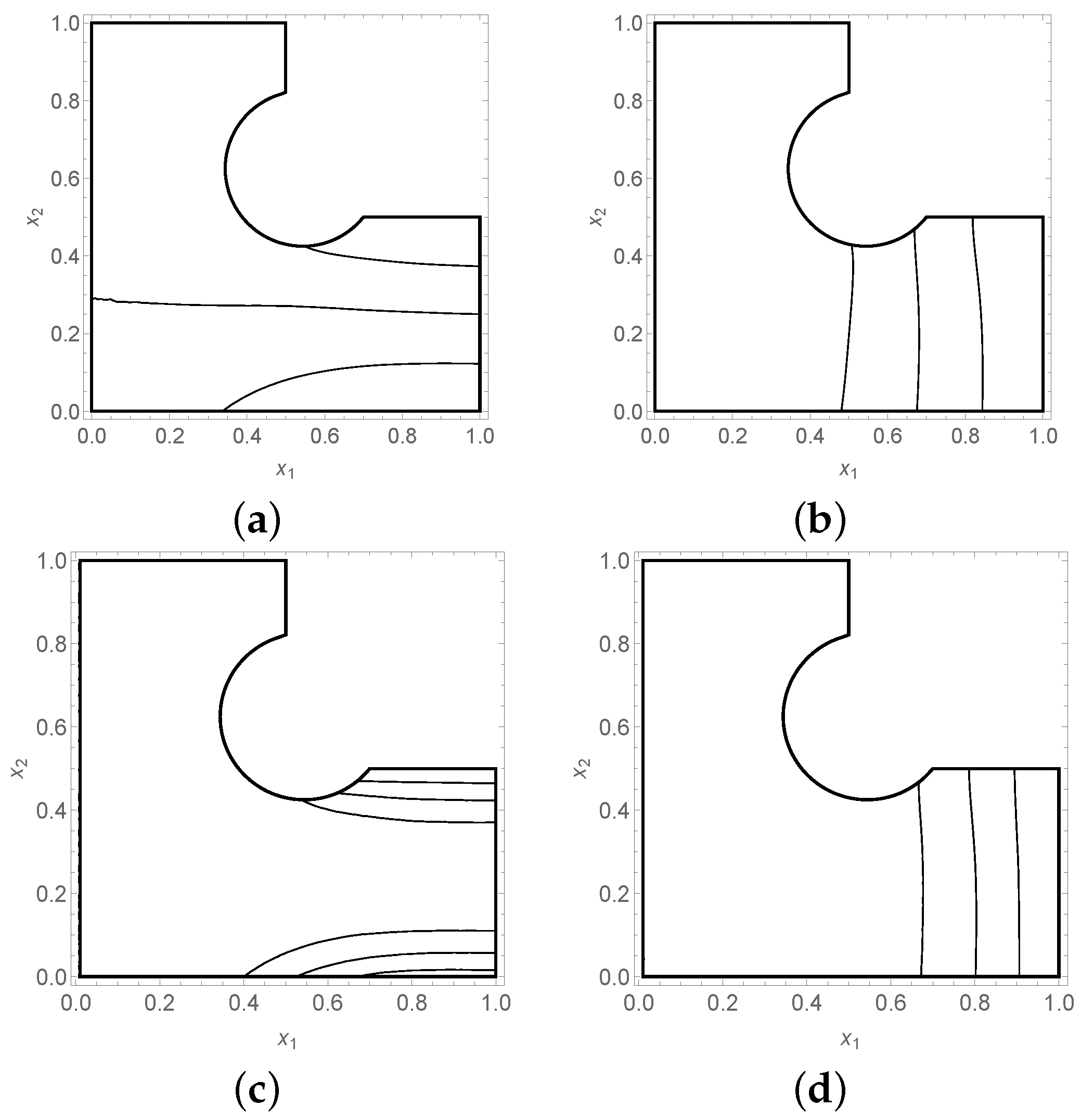
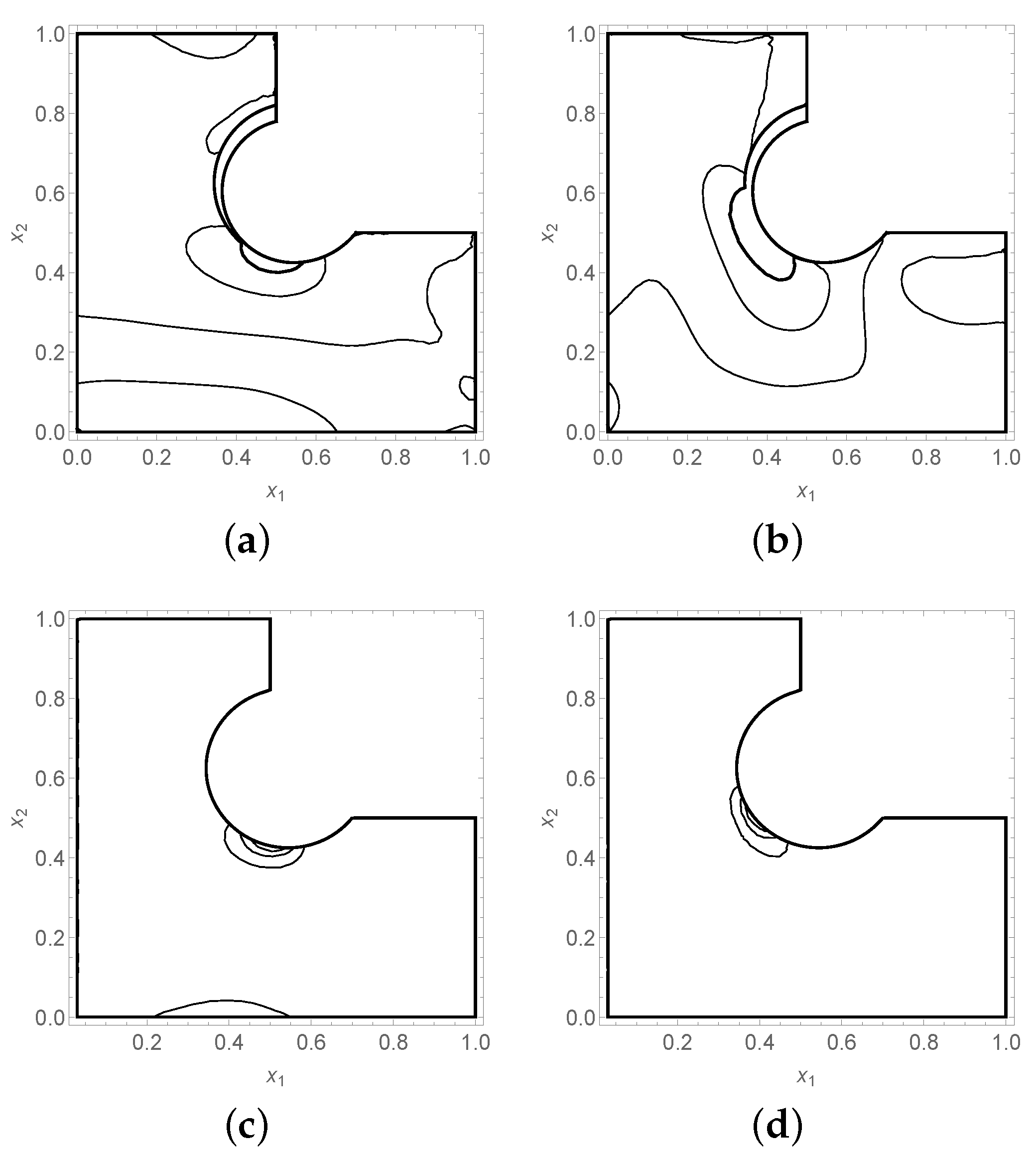
The potentials and two stress components are shown in Figure 6 and Figure 7. What sets these figures apart from the normal exposition is the inclusion of the variance plots. In particular, the information gained from the location of maximal variance is highly useful and in this case coincides with what one would expect in such a configuration. In particular, the variance in stresses is concentrated in the area where the moment due to loading is acting. This gives us high confidence in our results and the efficacy of the approach proposed here.

Of course, the proposed method only provides an approximation. In the current setting, the qualitative results obtained are accurate in the sense that visual comparison of the contour plots obtained with the two methods are indistinguishable. However, the errors in energy must translate to errors in norms of derived quantities.

6. Conclusions

Stochastic eigenvalue problems are nonlinear and multiparametric. They require their own solution methods and remain one of the challenge problems in computational mechanics. It turns out that planar elasticity on symmetric domains is the ideal setting for simplest possible reference problems, where the key is to have a cluster of eigenmodes at the low end of the spectrum.

In this paper, we have shown that the eigenvalue crossing can occur within clusters not only by perturbations of the domain, but also of material parameters. What is new is that in this setting, the crossing can be controlled; that is, the effect of the perturbations can actually be predicted.

Even though eigenvalue crossing means that identifying the smallest eigenpair is a difficult problem in multiparametric problems, the basis of the subspace is a well-defined concept and can be used for instance in low-rank approximation of solutions of problems with static loading. In our example, already with a relatively small number of collocation points, the reduction in solution times is significant.