Assessing Maize Yield Spatiotemporal Variability Using Unmanned Aerial Vehicles and Machine Learning

Abstract

Optimizing the prediction of maize (Zea mays L.) yields in smallholder farming systems enhances crop management and thus contributes to reducing hunger and achieving one of the Sustainable Development Goals (SDG 2—zero hunger). This research investigated the capability of unmanned aerial vehicle (UAV)-derived data and machine learning algorithms to estimate maize yield and evaluate its spatiotemporal variability through the phenological cycle of the crop in Bronkhorstspruit, South Africa, where UAV data collection took over four dates (pre-flowering, flowering, grain filling, and maturity). The five spectral bands (red, green, blue, near-infrared, and red-edge) of the UAV data, vegetation indices, and grey-level co-occurrence matrix textural features were computed from the bands. Feature selection relied on the correlation between these features and the measured maize yield to estimate maize yield at each growth period. Crop yield prediction was then conducted using our machine learning (ML) regression models, including Random Forest, Gradient Boosting (GradBoost), Categorical Boosting, and Extreme Gradient Boosting. The GradBoost regression showed the best overall model accuracy with R² ranging from 0.05 to 0.67 and root mean square error from 1.93 to 2.9 t/ha. The yield variability across the growing season indicated that overall higher yield values were predicted in the grain-filling and mature growth stages for both maize fields. An analysis of variance using Welch’s test indicated statistically significant differences in maize yields from the pre-flowering to mature growing stages of the crop (p-value < 0.01). These findings show the utility of UAV data and advanced modelling in detecting yield variations across space and time within smallholder farming environments. Assessing the spatiotemporal variability of maize yields in such environments accurately and timely improves decision-making, essential for ensuring sustainable crop production.

1. Introduction

Maize (Zea mays L.) is a crop of global significance and is especially important as a staple food for developing countries [1,2]. Globally, the maize crop has a harvested area of 234,291,525.8 hectares over six decades, from 1961 to 2021 [3]. The annual global average of maize yield stands at 5.8 t/ha, with developing countries producing a much lower average yield of 2.7 t/ha [4]. Since the 1960s, maize production in sub-Saharan Africa has increased mainly due to expanded cultivation, but smallholder farmers continue to face challenges in improving yields amid a growing population and rise in demand for food security [5]. The variability in maize yields in sub-Saharan Africa is due to several environmental and anthropogenic factors such as nutrients, sunlight, soil erosion, moisture, climatic variability, irrigation, planting techniques (e.g., strip tillage), tillage distance, and plough penetration of soils [6,7,8,9,10,11,12]. Declining maize yields are observed with the occurrence of extreme climatic events, e.g., high temperatures, droughts, and variability of climate modes, such as the El Niño–Southern Oscillation or the Indian Ocean Dipole [13,14]. Compared to smallholder farming, commercial farming uses optimal crop management techniques such as improved maize genetics and precision farming practices which encourage higher crop yields [4].

Accurate and timely information on crop growth conditions is vital for the reliable prediction of crop yields. This information assists in decision-making for crop management and resource allocation to farmers [15]. Several studies have demonstrated that non-intrusive data, processed through remote sensing techniques (such as satellite imagery), can provide both timely and accurate maize yield estimates [16,17,18,19]. Satellite images such as Sentinel-2, Landsat-8, and SPOT-4 have a lower than 5-m spatial resolution, and low revisit frequency, and can be contaminated by atmospheric clouds and their shadows that hinder crop modelling [20,21]. In recent years, the rapid development of unmanned aerial vehicle (UAV) technologies has increased their use for farm-level crop yield estimations as they allow for cost-effective data acquisition at high spatial resolutions [22,23,24]. The imagery assists in easily monitoring the complex phenology and structure of maize crops [25]. Recently, a study used UAVs for maize height, yield, and biomass predictions to assess the variability of crop development [26]. In that study, crop height estimations were employed in the generalized additive model for the prediction of dry grain yield with an accuracy of R² 0.90 [26].

The UAV data can produce spatial information about the crop which can be used for crop growth, crop yield, and health monitoring [27,28,29]. Recent UAV-based studies have focused on spectral, structural, and textural variables to predict phenotypic plant traits including plant height, canopy biomass, and grain yields [30,31,32,33]. Incorporating feature extraction techniques into UAV data can improve the study of maize crop phenology and in turn crop yield estimation. Schut et al. [34] used two vegetation indices (VIs), including the normalized difference vegetation index (NDVI) and the perpendicular vegetation index (PVI) derived from UAV and satellite images, to assess the effect of fertilizers on crop yields in smallholder fields. They reported that maize had the lowest correlation between relative yields and the coefficient of variation for the UAV-derived PVI with R² values as low as 0.21. These results show that using only two vegetation indices has the potential to hinder the prediction of crop yields. Similarly, the green NDVI (GNDVI) based on UAV imagery was found to produce a low predictor accuracy with the GNDVI (r < 0.4) when compared to measured maize yields [35]. Therefore, a variety of UAV-derived VIs need to be identified based on their correlation to maize yield for determining model inputs. Ramos et al. [36] identified 33 VIs and ranked the top three best-performing VIs when generating maize yield maps. They found that the three best VIs improved the prediction of maize yield with the RF algorithm; however, this approach was not effective with the other machine learning algorithms. Thus, identifying only a limited number of specific VIs for estimating crop yield might only be beneficial for some prediction algorithms. The study by Pinto et al. [37] reached similar conclusions, where best correlated VIs varied in effectiveness for yield predictions and the RF algorithm outperformed the other models. This improved accuracy of RF is most likely due to the ability of certain machine learning algorithms to handle complex non-linear relationships within data [38].

Textural features extracted from UAV data provide information such as contrast, mean, entropy, variance, homogeneity, dissimilarity, angular second moment, and correlation calculated from the grey-level co-occurrence matrix (GLCM) have the potential to improve maize crop yield estimations [39]. Yang et al. [40] effectively predicted maize yield at different phenological stages using both vegetation indices and GLCM-derived textural features. The results showed that UAV data produced R² values from 0.89 to 0.93. However, they observed that VIs were selected more frequently over the growing season than textural features when identifying the variables for yield prediction. Although VIs provide valuable insights into model accuracies, the integration of multiple datasets that incorporate textural features is imperative for maize yield predictions [41].

Many studies have combined UAV data and machine learning algorithms to predict maize crop yield [36,39,42,43,44]. For example, Danilevicz et al. [42] found that the multimodel deep learning model applied to UAV data predicted maize yield accurately at the early stage of development with an R² score of 0.73 and a root mean square error (RMSE) of 1.07 t/ha. In the study by Kumar et al. [43], machine learning models such as the k-nearest neighbour, support vector regression, and deep neural network were evaluated for maize yield prediction using UAVs. They found accuracies with R² ranging from 0.65 to 0.84 and a RMSE from 0.69 to 1.75 Mg/ha between the three models. Fan et al. [44] found that estimating maize yield with the UAV-mounted hyperspectral data produced low accuracies. They found that the ridge regression produced the highest values of the correlation coefficient (r = 0.54) and RMSE = 2.68. Bao et al. [45] also produced crop yield predictions from UAV-derived data and confirmed (with R² ranging from 0.860 to 0.898) that Gradient Boosting (GradBoost) outperformed traditional ordinary least squares and stepwise multiple linear regression. However, they found that the GradBoost model underestimated yield values, which was most likely due to small training samples and the high complexity of the model.

The availability of UAV-derived data for estimating spatiotemporal variability of maize yield is vital for assessing crop health. Monitoring yield over the crop development stages reveals growth patterns and informs optimized crop management. Sibanda et al. [46] achieved a high accuracy (R² = 0.95 and RMSE = 0.03) yield prediction for smallholder farmer maize using UAV data and the RF algorithm in the reproductive stages of the crop cycle. While the latter authors reported higher accuracy during the reproductive stages, another study in Zimbabwe found yield accuracy to be higher in the vegetative stages of crop development. These researchers showed that UAV data (red at the vegetative, near-infrared [NIR] at the vegetative stage, and red at the flowering stage) could accurately predict maize yield with r = 0.86 and RMSE = 0.323 [47]. In Ren et al. [48], the combination of UAV data from the entire growth period provided better yield predictions; however, the accuracies improved gradually from early to mature crop development. This indicated the importance of segregating the modelling exercise by growth stage [39,40,41,46,47,48]. Thus, there is a need to not only study the accuracy of the predictions but also to quantify the variation in predicted values throughout the season [39,40,41,46,47,48]. This can provide a better evaluation of the maize yield estimates at various phenological stages of the crop growth cycle.

The previous literature demonstrates that crop yield prediction accuracy depends significantly on the selected input variables, such as VIs and textural features (GLCM) [34,35,36,37]. Additionally, the performance of machine learning algorithms varies for maize yield prediction across the phenological cycle. Therefore, we propose an evaluation of different input features and machine learning algorithms to predict maize yield at the various stages of the crop cycle. The objectives of this study were as follows: (i) to identify the model input features based on the correlation between observed yield and UAV-derived spectra, VIs, and textural features; (ii) to evaluate the performance of machine learning algorithms for predicting maize yield at different growth stages; (iii) to assess feature importance for each algorithm; (iv) to create a yield map for the predicted maize estimates; and (v) to assess the spatiotemporal variability of yield estimates through the phenological cycle.

2. Materials and Methods

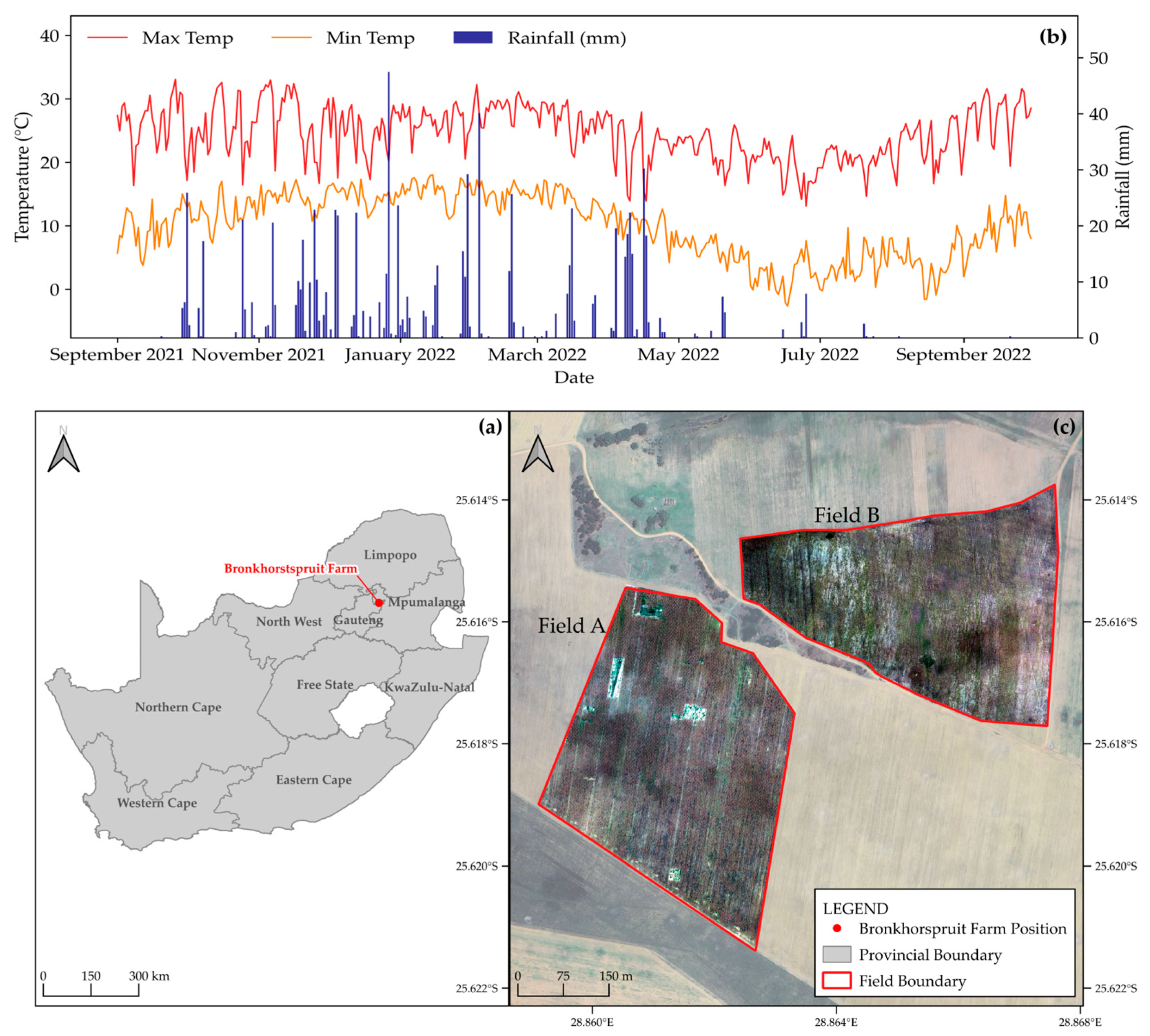
2.1. Study Site

The research was undertaken during the 2021/2022 maize growing season. The study used a medium-sized commercial farm comprising two fields, located in Bronkhorstspruit in the Tshwane Municipality, South Africa (Figure 1a). This study site was selected owing to the presence of smallholder farming areas such as in the nearby rural communities, thus offering a valuable comparative perspective on maize crop yields given similar environments. As the study region is part of the highveld ecoregion, the climate is characterized by rainy summers (from October to May) and dry winters. Figure 1b represents hourly temperature and rainfall data from the Bronkhorstspruit weather station at 25°42′07.5″ S 28°47’56.4″ E acquired from the Agricultural Research Council (ARC). The soil was predominantly sandy with an average of 2.92% soil moisture, based on 100 soil samples oven-dried at 105 °C taken in the study area. According to the 1:250,000 geological map published by the Council for Geoscience [49], the site is part of the Dwyka formation with a lithological description of tillite and shale. The two different maize varieties had been planted, namely white maize in Field A and yellow maize in Field B (Figure 1c). Generally, the maize crop has a life cycle that varies depending on the planting date and locality of the site. The life cycle of the maize plant was found to extend 120 to 160 days on average [50] and had been planted in November. The life cycle of maize consists of the vegetative and reproductive growth stages. The vegetative stage includes the initial seedling emergence (VE), leaf growth (V1-V14), and tasselling (VT). The reproductive stage includes silking (R1), blistering (R2), milking (R3), dough (R4), dent (R5), and physiological maturity (R6) [51].

2.2. Field Yield Measurements

A field visit was conducted over 18–21 May 2022 for the collection of in situ yield measurements at the study site. Prior to the field visit, a systematic grid consisting of 200 sampling points was created, allocating 100 points for each field. The objective yield survey methodology described by Bernardi et al. [52] (developed for estimating the yields of white and yellow maize) was adopted in this study. At each designated sampling point, a 10-m section of the row was selected for assessment. Here, ears of maize were counted and arranged in order of ear size, from shortest to longest. The median ear was then chosen for further analysis; it was shelled and weighed, and the moisture content was determined. Additionally, the width of the maize row was measured across a span of six rows. Using these data, yield estimates were calculated using a regression model that included a bias correction factor for ensuring accurate yield estimates. Not all of the 200 sampling points collected per month were suitable for machine learning to model data for estimating crop yields (specifically, only 194 points were usable for January and February, respectively, 188 for April, and 199 for May of 2022). The life cycle of the maize plants broadly reached the pre-flowering stage in January, flowering in February, grain-filling in April, and maturity by May 2022.

2.3. Remote Sensing Imagery and Preprocessing

Images were acquired using UAVs on 26 January, 23 February, 6 April, and 18 May 2022, coinciding with the field survey and the four growing stages (pre-flowering, flowering, grain-filling, and maturity) of the maize crop in the area. The UAV system used was the Matrice 600 Pro product by the DJI company. Images were collected with the DLS 2 light sensor with an integrated Global Positioning System (GPS). The commercial MicaSense RedEdge-MX multispectral camera was used [53]. The UAV images were acquired at an 8 cm resolution with spectral bands including red (663–673 nm), green (550–570 nm), blue (465–485 nm), red-edge (712–722 nm), and NIR (820–860 nm) bands, with a horizontal field of view of 47.2°. The output of the five narrow spectral band images consisted of a 12-bit raw digital output format. The UAV flight height was set to 120 m in favourable atmospheric conditions that guaranteed high-accuracy point cloud data and image acquisition. The raw radiometric data were processed in a three-step process using the photogrammetry software called Pix4Dmapper 4.8.0 version (Pix4D, Lausanne, Switzerland). This process includes the following: (i) initial processing by correcting image orientation and georeferencing the images based on ground control points; (ii) the computation of dense point cloud and 3D calculated mesh; and (iii) the creation of the digital surface model, orthomosaic, and index map. Radiometric corrections for raw images were performed using Pix4Dmapper; before the flight commences, a picture is captured to calibrate the imagery from a target panel for radiometric correction using a reference panel with known properties, such as the position of the sun and irradiance. The Pix4Dmapper produced geotiff image outputs for each spectral band for this study.

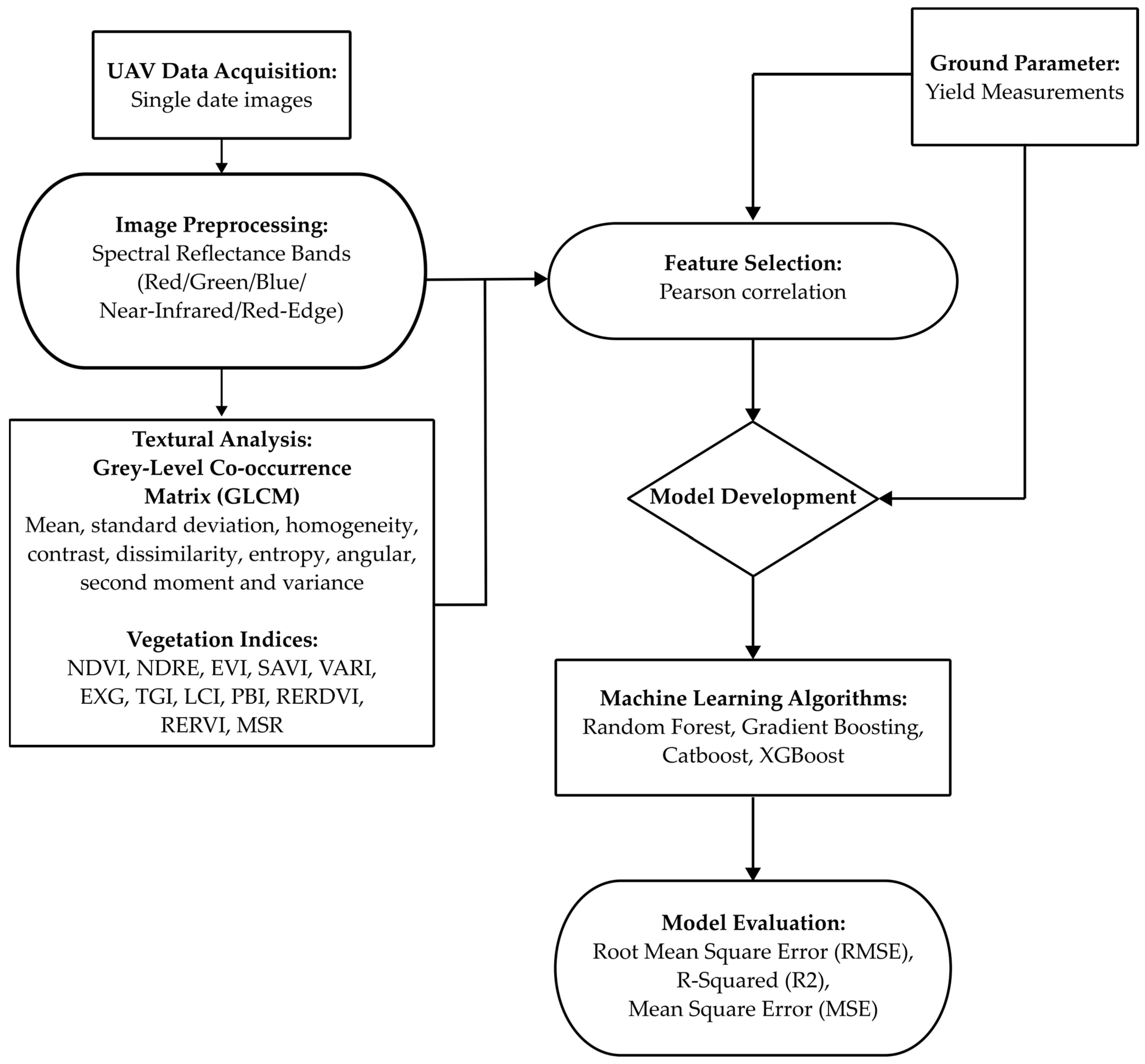
2.4. An Overview of the Methodology

The overall workflow for the methodology is illustrated in Figure 2; this mainly consisted of the following: (i) collection of UAV imagery; (ii) image preprocessing of the spectral reflectance data; (iii) analysis of spectral data for calculating the textural features and vegetation indices; (iv) the selection of correlated features with yield measurements; (v) creating a model for predicting maize yield from the UAV input data; and (vi) evaluating model accuracy and performance for predicting yield.

2.4.1. Textural Properties

The GLCM statistical technique is widely used for extracting vital textural features for studying crop structure and yields. It is needed to detect variations in texture that are related to changes in crop health, density, and development. In this study, the GLCM was implemented using the ‘glcm’ package available in R software (Version 4.3.3) [54]. Seven textural features were calculated from the red, green, and blue spectral bands: mean, homogeneity, dissimilarity, entropy, angular second moment, variance, and contrast (Table 1).

2.4.2. Spectral Vegetation Indices

Vegetation indices (VIs) play a pivotal role in quantifying plant health indicators, including photosynthetic activity, chlorophyll presence, biomass, and soil properties [29,55,56,57,58,59]. Their application extends to evaluating key growth attributes and potential yields of the crop. In this study, 12 VIs that are widely used in vegetation characterization were explored (Table 1). The VIs were chosen based on their specific capability to identify distinct aspects of the crop in terms of sensitivity to changes in soil background; they decrease the saturation effect of NDVI, they enhance the green vegetation signal, and they are sensitive to chlorophyll content [29,55,56,57,58,59]. These VIs were computed using Python (3.12.4).

Table 1. Description of selected textural features and vegetation indices.

Features	Formula	References
$\left(i,j\right)$th entry in normalized grey-tone spatial dependence matrix	$p\left(i,j\right)$	Haralick et al. [60]
The distinct number of grey levels in the image	$N_g$
$\mathrm{Mean}\mathrm{of}{p}_x$$\mathrm{and}{p}_y$	$\mu$
Mean	${\displaystyle \sum _i}{\displaystyle \sum _j}x\left(i,j\right)p\left(i,j\right)$
Homogeneity	${\displaystyle \sum _i}{\displaystyle \sum _j}\frac{1}{1+{\left(i-j\right)}^2}p\left(i,j\right)$
Dissimilarity	${{\sum }_{n=1}^{N_g-1}n\left\{{\sum }_{i=1}^{N_g}{\sum }_{j=1}^{N_g}p{\left(i,j\right)}^2\right\}}_{\left|i-j\right|=n}$
Contrast	${{\sum }_{n=0}^{N_g-1}{n}^2\left\{{\sum }_{i=1}^{N_g}{\sum }_{j=1}^{N_g}p{\left(i,j\right)}^2\right\}}_{\left|i-j\right|=n}$
Entropy	$-{\displaystyle \sum _i}{\displaystyle \sum _j}p\left(i,j\right)\log \left(p\left(i,j\right)\right)$
Angular second moment	${\displaystyle \sum _i}{\displaystyle \sum _j}{\left\{p\left(i,j\right)\right\}}^2$
Variance	${\displaystyle \sum _i}{\displaystyle \sum _j}{\left(i-\mu \right)}^{2}p\left(i,j\right)$
Leaf chlorophyll index (LCI)	$LCI=\frac{NIR-REdge}{NIR+R}$	Datt [61]
Excess green index (EGI/EXG)	$EXG=2\times \frac{G-R-B}{R+G+B}$	Woebbecke et al. [62]
Modified simple ratio (MSR)	$MSR=\frac{\left(\frac{NIR}{R}\right)-1}{\sqrt{\frac{NIR}{R}+1}}$	Chen [63]
Red-edge re-normalized difference vegetation index (RERDVI)	$RERDVI=\frac{NIR-REdge}{\sqrt{NIR+REdge}}$	Cao et al. [64]
Plant biochemical index (PBI)	$PBI=\frac{NIR}{G}$	Rao et al. [65]
Red-edge ratio vegetation index (RERVI)	$RERVI=\frac{NIR}{REdge}$	Jasper et al. [66]
Visible atmospheric resistant index (VARI)	$VARI=\frac{G-R}{G+R-B}$	Gitelson et al. [67]
Triangular greenness index (TGI)	$TGI=-\frac{190\left(R-G\right)-120\left(R-B\right)}{2}$	Hunt Jr et al. [68]
Normalized difference vegetation index (NDVI)	$NDVI=\frac{\left(NIR-R\right)}{\left(NIR+R\right)}$	Tucker [69]
Enhanced vegetation index (EVI)	$EVI=2.5\times \frac{\left(NIR-R\right)}{\left(NIR+6R-7.5B+1\right)}$	Huete et al. [70]
Soil-adjusted vegetation index (SAVI)	$SAVI=\frac{(1+0.5) \times (NIR-R)}{(NIR+R+0.5)}$	Huete [71]
Normalized difference red-edge index (NDRE)	$NDRE=\frac{\left(NIR-REdge\right)}{\left(NIR+REdge\right)}$	Barnes et al. [72]

Table 1. Description of selected textural features and vegetation indices.

Features	Formula	References
$\left(i,j\right)$th entry in normalized grey-tone spatial dependence matrix	$p\left(i,j\right)$	Haralick et al. [60]
The distinct number of grey levels in the image	$N_g$
$\mathrm{Mean}\mathrm{of}{p}_x$$\mathrm{and}{p}_y$	$\mu$
Mean	${\displaystyle \sum _i}{\displaystyle \sum _j}x\left(i,j\right)p\left(i,j\right)$
Homogeneity	${\displaystyle \sum _i}{\displaystyle \sum _j}\frac{1}{1+{\left(i-j\right)}^2}p\left(i,j\right)$
Dissimilarity	${{\sum }_{n=1}^{N_g-1}n\left\{{\sum }_{i=1}^{N_g}{\sum }_{j=1}^{N_g}p{\left(i,j\right)}^2\right\}}_{\left|i-j\right|=n}$
Contrast	${{\sum }_{n=0}^{N_g-1}{n}^2\left\{{\sum }_{i=1}^{N_g}{\sum }_{j=1}^{N_g}p{\left(i,j\right)}^2\right\}}_{\left|i-j\right|=n}$
Entropy	$-{\displaystyle \sum _i}{\displaystyle \sum _j}p\left(i,j\right)\log \left(p\left(i,j\right)\right)$
Angular second moment	${\displaystyle \sum _i}{\displaystyle \sum _j}{\left\{p\left(i,j\right)\right\}}^2$
Variance	${\displaystyle \sum _i}{\displaystyle \sum _j}{\left(i-\mu \right)}^{2}p\left(i,j\right)$
Leaf chlorophyll index (LCI)	$LCI=\frac{NIR-REdge}{NIR+R}$	Datt [61]
Excess green index (EGI/EXG)	$EXG=2\times \frac{G-R-B}{R+G+B}$	Woebbecke et al. [62]
Modified simple ratio (MSR)	$MSR=\frac{\left(\frac{NIR}{R}\right)-1}{\sqrt{\frac{NIR}{R}+1}}$	Chen [63]
Red-edge re-normalized difference vegetation index (RERDVI)	$RERDVI=\frac{NIR-REdge}{\sqrt{NIR+REdge}}$	Cao et al. [64]
Plant biochemical index (PBI)	$PBI=\frac{NIR}{G}$	Rao et al. [65]
Red-edge ratio vegetation index (RERVI)	$RERVI=\frac{NIR}{REdge}$	Jasper et al. [66]
Visible atmospheric resistant index (VARI)	$VARI=\frac{G-R}{G+R-B}$	Gitelson et al. [67]
Triangular greenness index (TGI)	$TGI=-\frac{190\left(R-G\right)-120\left(R-B\right)}{2}$	Hunt Jr et al. [68]
Normalized difference vegetation index (NDVI)	$NDVI=\frac{\left(NIR-R\right)}{\left(NIR+R\right)}$	Tucker [69]
Enhanced vegetation index (EVI)	$EVI=2.5\times \frac{\left(NIR-R\right)}{\left(NIR+6R-7.5B+1\right)}$	Huete et al. [70]
Soil-adjusted vegetation index (SAVI)	$SAVI=\frac{(1+0.5) \times (NIR-R)}{(NIR+R+0.5)}$	Huete [71]
Normalized difference red-edge index (NDRE)	$NDRE=\frac{\left(NIR-REdge\right)}{\left(NIR+REdge\right)}$	Barnes et al. [72]

2.5. Feature Selection

In this study, the Python library ‘pandas’ was used to analyse the correlations between the measured maize yield data and the spectral input features described in Section 2.4.1 and Section 2.4.2. This is performed before regression analysis for feature selection and ensures only the highest correlated features are included in the modelling process. The Pearson correlation coefficient (r) was used for identifying the correlated features. Features that correlated well with maize yield (moderate to substantial r values ranging between r > 0.5 and −0.65) were selected for each year to run regression analysis to produce prediction models [20,73,74,75].

Furthermore, the recursive feature elimination with cross-validation (RFECV) was applied to each model to select non-collinear features and avoid redundancy. This process identifies the best subset of features that most significantly contribute to model performance. The RFECV ensures that the least important features are removed before evaluating the model’s performance based on cross-validation scores at each iteration. The Python library, Scikit-learn, was used to apply RFECV with the following parameters: 10-fold cross-validation; R² for scoring each feature; and a minimum threshold of ten features.

2.6. Machine Learning Algorithms

Four machine learning algorithms were selected for this study, namely RF, Extreme Gradient Boosting (XGBoost 2.1.0), GradBoost (0.20), and Categorical Boosting (CatBoost 1.2.5). These algorithms were implemented in Python using their respective libraries. Hyperparameter optimisation was completed for this study to determine the best parameters for each model. In the current study, the grid search method was chosen for the fine-tuning and optimisation of parameters. GridSearchCV (1.5.0) is the specific method from Scikit-learn that was used to systematically evaluate combinations of the model parameters using the 10-fold cross-validation, thus optimising the R² metric.

The RF regression is a supervised machine learning algorithm that is available for the prediction of continuous data. For improved accuracy, RF creates a forest of decision trees using a random subset of training data. Each tree consists of a prediction which is used to create a final prediction based on the average values from all the individual tree predictions [76]. The processing of the algorithm was coded using the Scikit-learn library in Python [77].

The GradBoost regression algorithm is an ensemble learning technique that makes predictive models [78]. Decision trees are created using an iterative procedure that starts with weak learners. The aim is to create strong learners by reducing the pseudo residual values (the difference between the observed and predicted values). Each tree is added to minimize the loss function which is defined initially at the start of the process. Therefore, each tree is trained to predict values that can reduce the error between observed and predicted values. The processing of this algorithm was completed in the Scikit-learn Python library [77].

The XGBoost regressor is a machine learning algorithm known for improving decision trees (tree boosting) to create an ensemble learning algorithm [79]. XGBoost uses the principles of GradBoost to create the models sequentially to reduce the residuals of each of the decision trees. This model is further optimized by parallelized tree building. Tree pruning is also performed in a backwards direction by calculating the difference between the calculated gain from similarity scores and the user-defined gamma (or tree complexity) parameter. XGBoost also incorporates regularization (L1-Lasso and L2-Ridge regression) to balance the model’s bias and variance, which controls model complexities and prevents overfitting. The processing of this algorithm was completed using the XGBoost library in Python.

The CatBoost machine learning algorithm is another algorithm that uses decision trees with categorical data and the framework of GradBoost. CatBoost uses symmetric trees which is unique to this algorithm, which means that all the nodes are split exactly the same at all depths. This is carried out to avoid overfitting and to reduce computing times [80]. The CatBoost Python library was used for modelling this algorithm.

2.7. Accuracy Assessment

The following statistical metrics were used to assess the model performance in this study: (i) R², (ii) RMSE, (iii) mean square error (MSE), and (iv) the relative RMSE (RRMSE). Formulas (1)–(4) are given below:

$$R^2=1-\frac{\sum _{i=1}^N{\left(y_i-{\widehat{y}}_i\right)}^2}{\sum _{i=1}^N{\left(y_i-{\overline{y}}_i\right)}^2},$$

(1)

$$RMSE=\sqrt{\frac{\sum _{i=0}^N{\left(y_i-{\widehat{y}}_i\right)}^2}{n-1}},$$

(2)

$$MSE=\frac{\sum _{i=1}^N{\left(y_i-{\widehat{y}}_i\right)}^2}{n},$$

(3)

$$RRMSE=\frac{RMSE}{{\overline{y}}_i}\times 100\%,$$

(4)

where, $n$ is the sample size or number of data points, $y_i$ is the observed yield values, ${\overline{y}}_i$ is the mean value of all the observed yields, and the ${\widehat{y}}_i$ is the predicted yield value. In addition, $N$ is the total number of data points in the entire dataset.

Welch’s Analysis of Variance (ANOVA) was used to evaluate variations in maize yield across growth stages for Fields A and B [81]. The sample data (100 points per field) were randomly sampled from the predicted yield maize maps for each field. Welch’s ANOVA was chosen because (i) the data lacked homogeneity of the variances within each field, and (ii) the data were not normally distributed. This analysis involved four different dates, and for each date, the F-statistic and associated p-value were calculated using the ‘scipy.stats’ Python library.

3. Results

3.1. Correlation Analysis of Maize Yield and UAV Data for Feature Selection

Feature selection was explored by identifying the correlation between maize yield and feature variables. The Pearson correlation coefficient was used to evaluate the correlation between maize yield and the spectral bands, GLCM-derived textural features, and VIs from UAV-derived data. Figure 3 shows the correlation data between the 41 spectral feature bands and maize yield over the four months. The correlation between maize yield and the UAV spectral data for January 2022 is shown in Figure 3a. A moderate correlation coefficient threshold of r > 0.5 was specified for feature selection to identify the top correlated bands for this month [20,82]. Most prominently, the PBI vegetation index showed the highest correlation with yield with r = 0.57. The LCI, NDRE, and RERVI were the second-highest correlated features with r = 0.56.

In February 2022, a moderate correlation coefficient threshold of r > 0.5 was adopted for feature selection, resulting in the selection of ten bands (Figure 3b) for inclusion in model prediction. The RERDVI vegetation index had the highest correlation at r = 0.71, followed by the RERVI (r = 0.69) and the NDRE (r = 0.68). The latter two features were quantified using the red-edge band.

The correlation between maize yield and spectral features for April 2022 is shown in Figure 3c. Notably, the correlation patterns in this dataset differ from the May 2022 data. In the initial phase of model training and testing for April, a substantial correlation of r > 0.65 was established, resulting in a total of 16 bands selected for analysis. Among these variables, the RERDVI exhibited the strongest correlation at r = 0.78, followed by an r = 0.77 for SAVI, RERVI, and MSR vegetation indices. The correlation results for this month favoured vegetation indices, with only one GLCM textural feature, specifically the red angular second moment, producing a correlation coefficient of r = 0.67 and selected for model input.

In the May 2022 dataset, the 11 features showing the highest correlation with yield were textural (GLCM) (Figure 3d). The GLCM features, including green mean, red mean, and red variance had the highest correlation with crop yield (r = 0.72). To diversify the spectral feature types to be used in a further regression analysis, the correlation threshold was relaxed by specifying it at 0.6. This specification resulted in the selection of 22 features that also included vegetation indices (PBI, SAVI, and EVI).

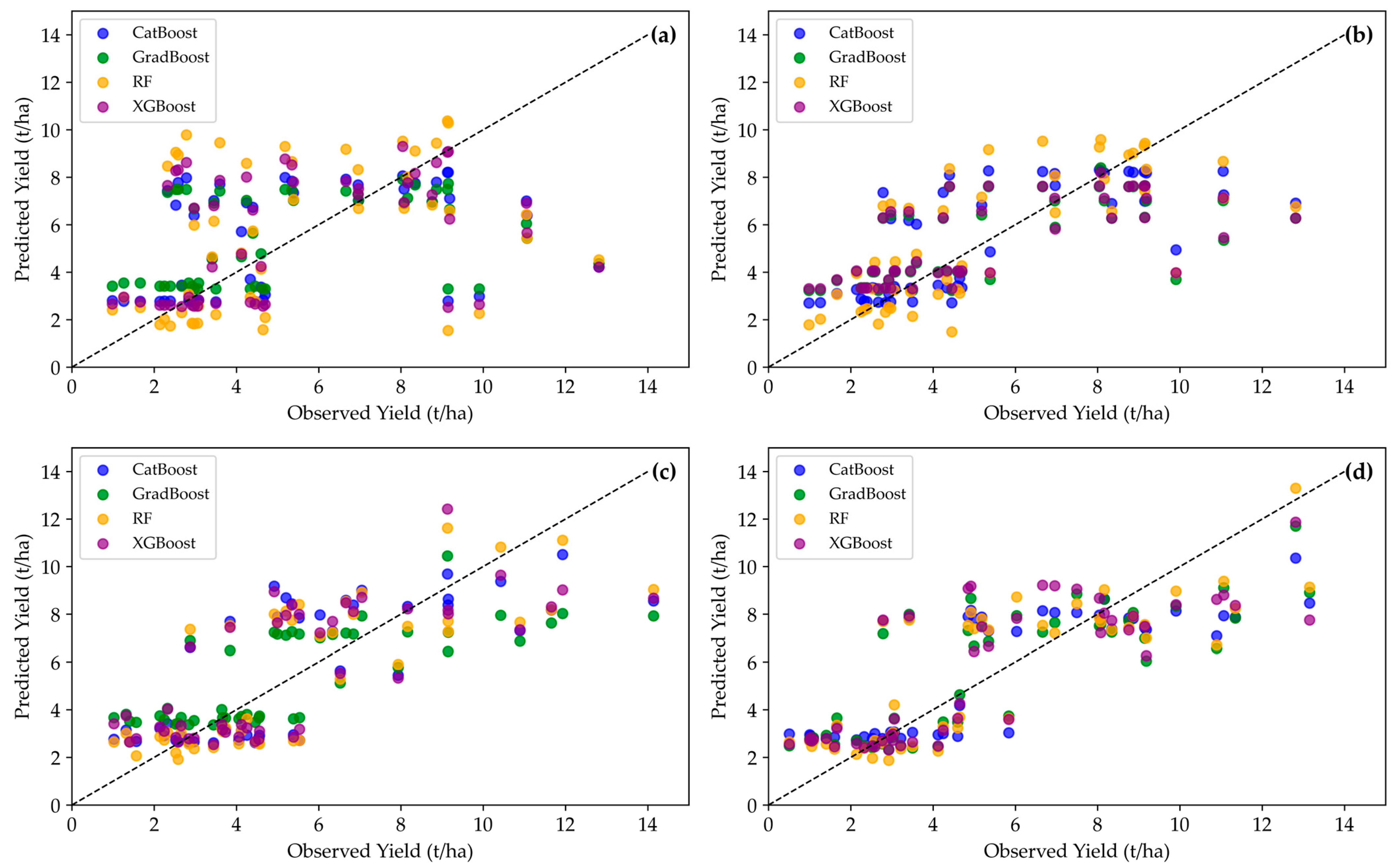
3.2. Development of Maize Yield Prediction Models

To assess the predictive performance of the machine learning models and determine their accuracy in yield estimation, we trained and tested four machine learning models: CatBoost, GradBoost, RF, and XGBoost. For optimization of the algorithm, fine-tuning of hyperparameters was needed. For RF this included the number of decision trees (n_estimators = 100, 200, 300), the maximum depth of each tree (max_depth = None, 5, 10), and the minimum samples required to split the node (min_sample_split = 2, 5, 10). For GradBoost, the hyperparameter tuning included n_estimators = 100, 200, 300; max_depth = 3, 5, 7; and the learning_rate = 0.01, 0.1, 0.3. The learning_rate is a parameter that determines the size of the contribution of each decision tree to the final prediction, i.e., 0.3 results in a 70% decrease in the contribution of each tree. The hyperparameter tuning for XGBoost included n_estimators = 100, 200, 300; max_depth = 3, 5, 7; and the learning_rate = 0.01, 0.1, 0.3. Lastly, the hyperparameter tuning for the CatBoost algorithm consisted of n_estimators = 100, 200, 300; max_depth = 3, 5, 7; and the learning_rate = 0.01, 0.1, 0.3.

Four statistical metrics were used in the evaluation of the proposed prediction models. These models were evaluated to determine the lowest error in the yield predictions. Figure 4 shows the model results using the metrics for the four phenological stages. The R² values for the RF algorithm ranged from −0.32 to 0.68 (Figure 4a); thus, this model produced both the lowest accuracy and highest R² score. The R² values for the GradBoost algorithms ranged from 0.05 to 0.67. This was followed by the CatBoost algorithm where R² values ranged between 0.06 and 0.64. The lowest values were observed for the XGBoost algorithm, and the values ranged from −0.1 to 0.63. The graph shows that the four algorithms performed the worst during the pre-flowering stage of maize growth, especially the low values observed from the RF and XGBoost algorithms. The R² values for the grain-filling and mature growth stages were the highest for the RF and GradBoost algorithms, which makes it difficult to choose one model over another.

Figure 4b shows the RMSE results for the four algorithms, with the RMSE values for the GradBoost algorithm ranging from 1.93 to 2.9 t/ha. In comparison, the CatBoost algorithm observed RMSE values between 2.00 and 2.89 t/ha, and the XGBoost algorithm showed values ranging from 2.04 to 3.12 t/ha. The RMSE values for the RF algorithm spanned from 1.90 to 3.42 t/ha.

The MSE values were the lowest for the GradBoost algorithm, as values ranged from 3.74 to 8.41 t/ha for the four time periods. The graphs showed that this was followed by the CatBoost algorithm, which showed similar lower MSE values ranging between 4.01 and 8.33 t/ha. The higher MSE values were shown to be from the XGBoost algorithm, with values ranging from 4.15 to 9.72 t/ha. The highest MSE values were found in the RF algorithm results, where values ranged between 3.62 and 11.66 t/ha (Figure 4c).

Similar trends were seen for RMSE and MSE values on the one hand, and R² on the other hand. However, for the flowering growth stage, the CatBoost algorithm produced slightly improved results compared to the three other models. The RF and GradBoost models overall produced consistently favourable values for all three metrics (R², RMSE, and MSE). This is further confirmed by the 1% difference between the RRMSE values for the flowering, grain-filling, and maturity stages, with the GradBoost producing 10% less error than the RF based on the RRMSE for the pre-flowering stage. Based on our study, these algorithms can be considered the most satisfactory algorithms for maize yield estimation.

Figure 5 represents the scatterplots of maize yield estimations; the scatterplots indicate the performance of the four machine learning models by comparing the linear correlation of prediction yield values to the observed values across the growth stages. The algorithms produced results that were overestimated in most low-yield cases. The data points in Figure 5a showed the most variation for all the models with values plotting significantly above or below the trendline. The RF algorithms for the pre-flowering phase produced the most under- and overestimated yield values. Figure 5b shows an improvement in the linear fitting between the observed and predicted yield values. XGBoost predicted yield that deviated significantly from the 1:1 trendline during the flowering (Figure 5b) and grain-filling (Figure 5c) growth stages. The GradBoost, RF, and CatBoost algorithms exhibited similar trends, with data points indicating a good linear fit as points closely aligned with the trendline. This indicates the efficiency of the algorithms to estimate maize yield. The highest accuracy relative to the 1:1 reference line (with data points closely clustered around) was for the grain-filling and mature stages of crop development. This suggests the models performed the best for maize yield estimations for these periods.

The cross-validation results for the four models are shown in Figure 6. The boxplots show variations in the metrics R², RMSE, and MSE for the four machine learning algorithms. Based on the higher R² values and lower RMSE and MSE values, better predictive accuracies were generally obtained for the flowering, grain-filling, and mature growth stages compared to pre-flowering.

Table 2. Summary of cross-validation accuracy of predicted yield models.

Model Type	Life Cycle	Training R2 Score	Test R2 Score	Cross-Validation Mean R2	Cross-Validation Mean RMSE	Cross-Validation Mean MSE
CatBoost	Pre-flowering	0.52	0.06	0.42	2.78	8.23
CatBoost	Flowering	0.58	0.55	0.49	2.60	7.12
CatBoost	Grain filling	0.69	0.56	0.49	2.48	6.55
CatBoost	Maturity	0.71	0.64	0.53	2.46	6.58
GradBoost	Pre-flowering	0.56	0.05	0.36	2.93	9.11
GradBoost	Flowering	0.61	0.43	0.45	2.73	7.86
GradBoost	Grain filling	0.69	0.54	0.41	2.69	7.76
GradBoost	Maturity	0.88	0.67	0.49	2.54	6.85
RF	Pre-flowering	0.79	−0.32	0.36	2.88	8.81
RF	Flowering	0.82	0.47	0.42	2.85	7.66
RF	Grain filling	0.88	0.56	0.43	2.49	6.54
RF	Maturity	0.85	0.68	0.50	2.52	6.77
XGBoost	Pre-flowering	0.70	−0.10	0.37	2.88	8.74
XGBoost	Flowering	0.59	0.44	0.45	2.71	7.73
XGBoost	Grain filling	0.82	0.52	0.42	2.53	6.96
XGBoost	Maturity	0.86	0.63	0.51	2.49	6.66

shows the metrics for the models to evaluate the performance further in terms of the training, testing, and the mean R² cross-validation results. In Figure 6, the CatBoost showed the model performance was the best across all the models and periods. The majority of higher R² values were concentrated within the 75th percentile for the pre-flowering and mature growth stages, as indicated by the median lines. The CatBoost produced the best range of mean R² cross-validation values ranging from 0.42 to 0.53. This algorithm also produced low RMSE (2.46 to 2.78 t/ha) and MSE (6.58 to 8.23 t/ha) cross-validation values. The other models did not produce significantly lower results. The XGBoost algorithm produced cross-validation results with mean R² cross-validation results ranging from 0.37 to 0.51. The mean RMSE ranged between 2.49 and 2.88 t/ha and the mean MSE ranged between 6.66 and 8.74 t/ha. The median values of the XGBoost-based results were similar to the GradBoost and RF algorithms. The RF algorithm produced a mean R² ranging between 0.36 and 0.50. The mean RMSE ranged between 2.52 t/ha and 2.88 t/ha, and the mean MSE ranged between 6.77 t/ha and 8.81 t/ha. The results for the GradBoost algorithm for the four time periods showed cross-validation mean R² values ranging from 0.36 to 0.49. This algorithm produced mean RMSE ranging from 2.54 to 2.93 t/ha and the MSE for this algorithm ranged from 6.85 to 9.11 t/ha. In comparison to the CatBoost, RF, and XGBoost algorithms, the GradBoost algorithm had the highest overall error range.

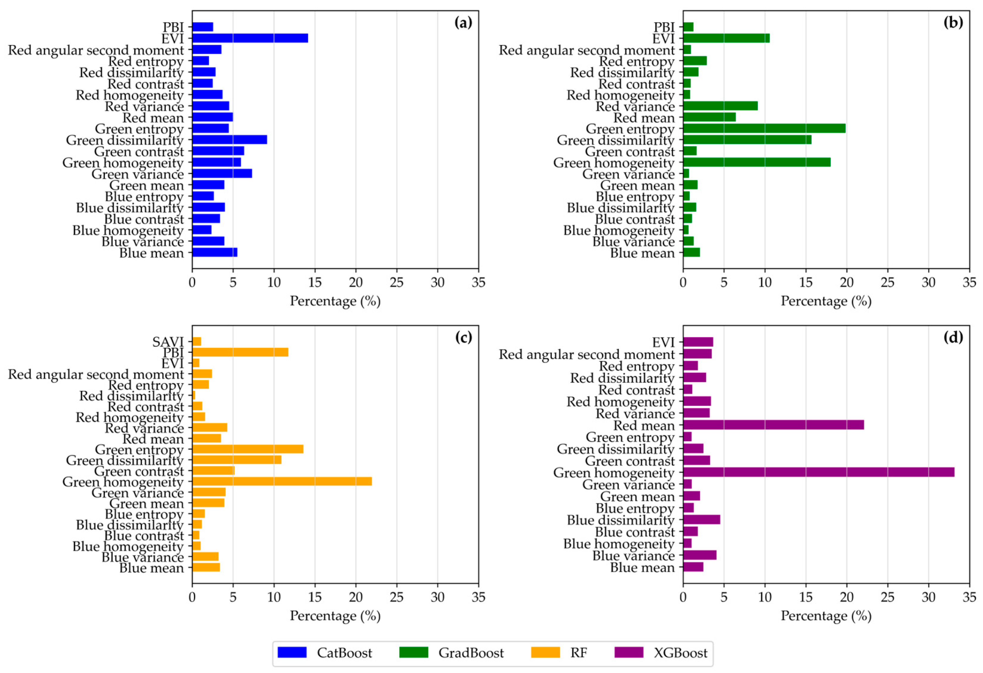
3.3. Input Features of Importance for Maize Yield Prediction

The significance of various input features in predicting maize yield using the four machine learning regression models is shown in Figure 7, based on the UAV data collected for the maturity growth stage. Figure 7a shows that the EVI had the highest importance in predicting maize yield when the CatBoost model was used. This feature also made a significant contribution to the prediction for the GradBoost (Figure 7b) and RF (Figure 7c) algorithms, where the feature had the fourth-highest importance value for those models. The green-derived textural features ranked the highest for the GradBoost, RF, and XGBoost algorithms (Figure 7b–d). Green dissimilarity and green variance produced the second-highest and third-highest variable importance in the CatBoost algorithm (Figure 7a) in predicting maize yield. The importance of the textural bands is especially observed in the RF model, where green homogeneity ranked first, green entropy ranked second, PBI ranked third, and green dissimilarity ranked fourth. The XGBoost model showed that two textural features, namely green homogeneity and red mean, had markedly more significance than the other features (Figure 7d). The remaining features had relatively low significance (with a contribution of <5%) (Figure 7d).

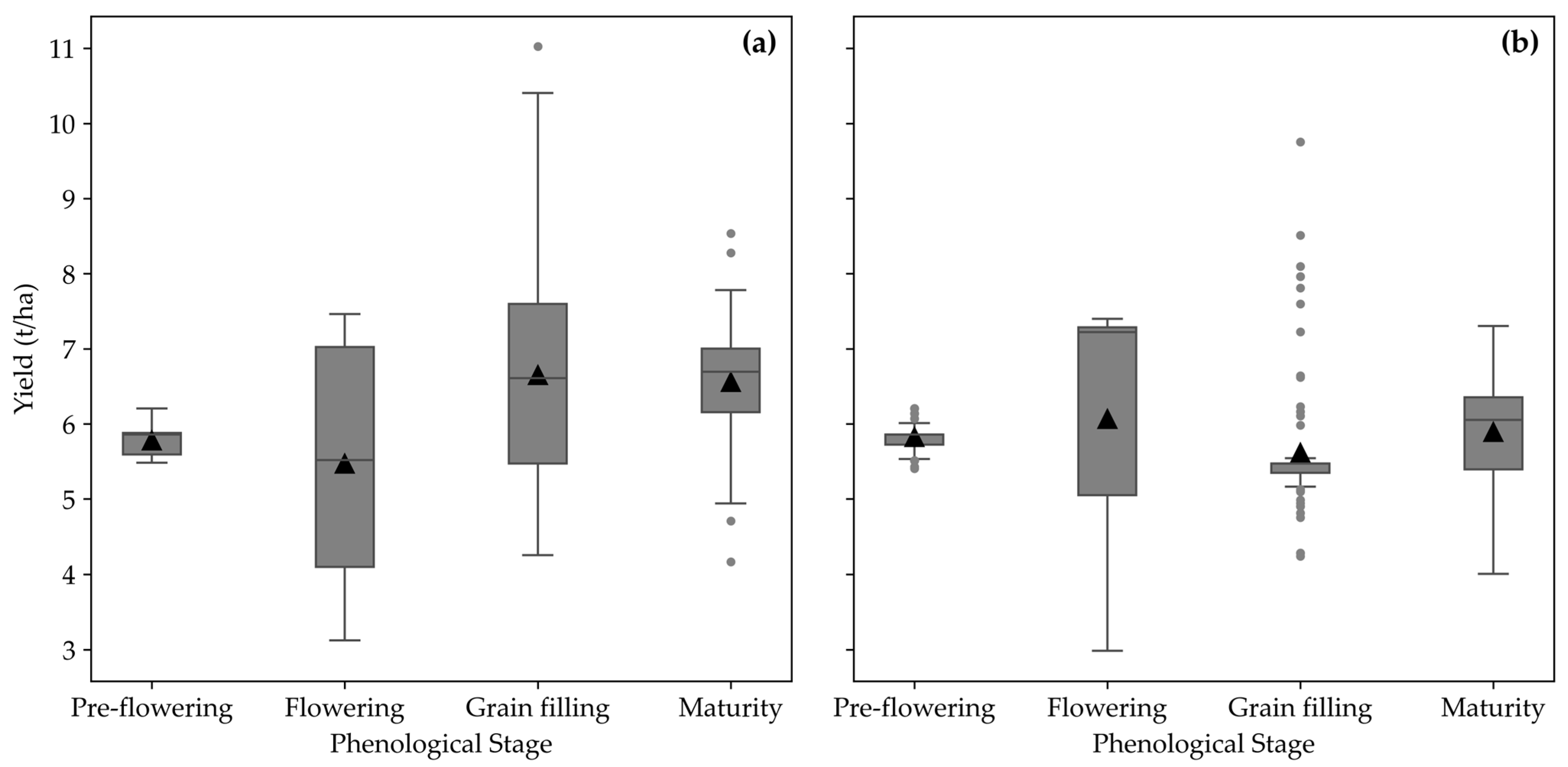
3.4. Visualizing Temporal Analysis of Maize Yield Variability

The previous section produced varying levels of model performance, with the GradBoost algorithm generally yielding favourable model performance, compared to the other models. Figure 8a is a map of the observed yield values visualized with inverse distance-weighted (IDW) interpolation. Maize yield maps generated using the GradBoost regression predictions for four growth periods in 2022 provide valuable insights into the variability of maize yield for the monitored fields. The yield distribution maps are generally heterogeneous on each date, thus highlighting the importance of maps in representing the spatiotemporal variability of maize yield. Figure 8b shows maize yield estimates at the pre-flowering stage of maize growth. The yield distribution is largely underestimated as shown on the pre-flowering map with Field A with a 5.68 t/ha or lower yield. At the flowering growth stage (Figure 8c), Field B had visibly higher yield estimates with large sections of the plot having a yield higher than 7.16 t/ha. In comparison, most areas of Field A had yield estimates below 5.68 t/ha for the same time. At the grain-filling stage (Figure 8d), yield estimates were considerably higher than the previous two dates. Field A showed a large area of the field with yield estimates greater than 8.64 t/ha and Field B showed estimates between 4.19 and 5.65 t/ha with a small section of the field to the west greater than 7.16 t/ha. The mature maize growth stage (Figure 8e) had yield estimates for Field A largely above 7.16 t/ha whereas Field B had a yield between 5.68 and 8.63 t/ha with sparse distribution across the field. These maps not only aid in assessing yield estimates but also offer valuable information for optimizing agricultural practices and resource allocation to maximize crop production.

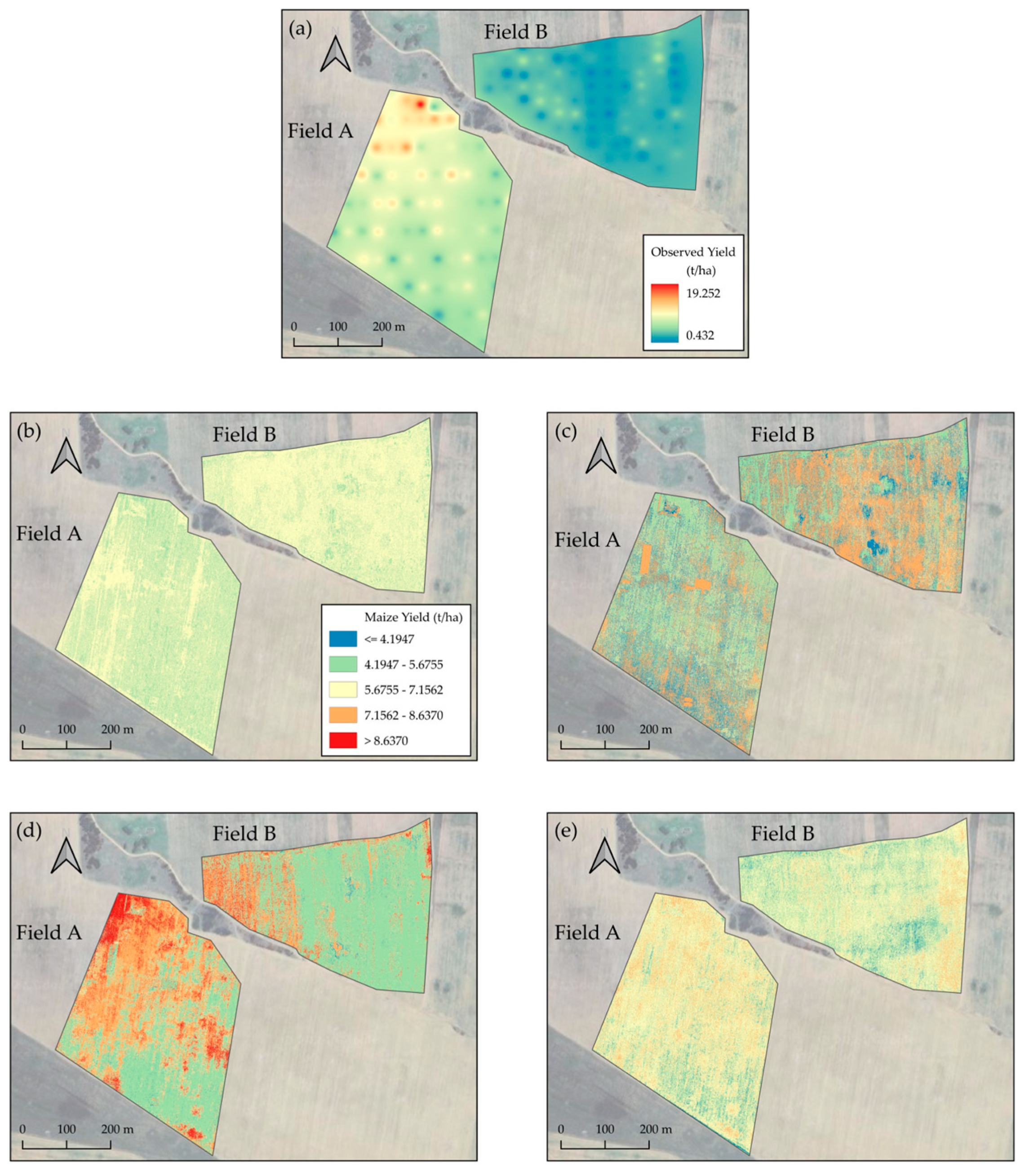
3.5. Maize Yield Spatiotemporal Variability

The maize yield estimates modelled using the GradBoost regression algorithm are represented as box plots in Figure 9 and are a comparative analysis between the four dates in 2022 for each field (Field A and Field B). Figure 9a provides clear results that show lower yield values for the pre-flowering and flowering growing stages for Field A. The grain-filling and mature stages had mean yield values (6.65 t/ha and 6.56 t/ha) that were higher than the mean values for the pre-flowering and flowering growth stages (5.76 t/ha and 5.47 t/ha) periods. Figure 9b shows that there are similar yield estimates predicted for all four stages of the maize growth for Field B. The mean values for the pre-flowering, flowering, grain-filling, and mature growth stages were 5.82, 6.07, 5.61, and 5.89 t/ha, respectively.

Table 3. Summary of Welch’s ANOVA results for yield comparison between different dates for Field A and Field B.

	Date 1	Date 2	F-Statistic	p-Value
Field A
	Pre-flowering	Flowering	3.99	0.047
	Pre-flowering	Grain filling	34.75	<0.001
	Pre-flowering	Maturity	109.49	<0.001
	Flowering	Grain filling	31.10	<0.001
	Flowering	Maturity	41.83	<0.001
	Grain filling	Maturity	0.30	0.58
Field B
	Pre-flowering	Flowering	2.14	0.15
	Pre-flowering	Grain filling	5.85	0.02
	Pre-flowering	Maturity	0.64	0.42
	Flowering	Grain filling	5.96	0.02
	Flowering	Maturity	0.91	0.34
	Grain filling	Maturity	5.59	0.02

presents the results of Welch’s ANOVA test to examine the difference in the predicted maize yield between different time periods for each field (Field A and Field B). The statistical analysis of Field A indicates that there was a high significant difference between the yield estimates, except for the comparison between the grain-filling and mature maize growth stages (with no significant difference of p = 0.583). Maize yield estimates were significantly different (p < 0.001) involving the grain-filling stage between the various growth stages in Field B. This suggests that Field A produced more consistent and significant changes over time. These findings highlight the importance of considering the temporal variability of evaluating crop yields in various fields when assessing crop health.

4. Discussion

This study evaluated the prediction of maize yield across four different maize growth stages. UAV imagery was used to extract features such as VIs and GLCM textural features from the RGB, red-edge, and NIR spectral bands. These feature bands were then assessed to determine the highest correlation between them and the measured maize yield. Pearson’s correlation coefficient was determined for the feature selection process and a correlation coefficient threshold identified the selected features for each dataset. The selected features were used as explanatory variables in four machine learning regression algorithms (RF, GradBoost, CatBoost, and XGBoost) to estimate maize yield. The models were then used to produce yield maps of the maize fields.

Feature selection is needed to identify the best features for yield estimation, and this process enhances regression modelling by reducing data redundancy. This ensures that the model only has the best possible feature inputs to improve model precision. Pearson’s coefficient allowed us to focus only on a selected number of features to be used as important inputs in the prediction process. The inclusion of multiple types of features proved to be more beneficial overall to improve yield prediction accuracy. The correlation values showed there was a difference in correlation level between different UAV-derived features and yield measured during the four months (Figure 3). This finding is in agreement with the study by Adak et al. [83], which found that using VIs at different growth stages is beneficial for predicting maize yield. This is due to different VIs being more sensitive to maize throughout the growing season [84,85].

The linear relationship between the predicted and observed maize crop yields shows prevalent underestimation and overestimation for the pre-flowering stage (Figure 5), indicating a lower yield prediction accuracy during the early stages. Higher prediction accuracies were during flowering, grain-filling, and the late grain maturity stages. During these stages, the characteristics of the crop change significantly with the intensity of greenness, chlorophyll concentrations, number of leaves, and plant height [29,86,87]. Therefore, the growth period can influence the capability of the UAV data to predict maize yield.

In this study, when comparing the performance of the regression algorithms, the accuracy of GradBoost (R² = 0.67) and RF (R² = 0.68) outperformed CatBoost and XGBoost. The authors Khanal et al. [88] reported that RF outperformed the other machine learning algorithms with a test R² score of 0.56, with the GradBoost model underperforming (R² = 0.43) for predicting maize yield. However, Du et al. [89] found that the GradBoost ensemble learning was shown to produce R² values of 0.799 compared to the RF model (R² = 0.749). The CatBoost algorithm has previously been shown to be successful in estimating crop yield [90,91]. The variations in accuracies between different machine learning algorithms are expected in studies related to maize yield predictions [17]. Differences in the performance of these models from one study to another can be a result of a range of factors such as environment, climate, maize genotype, time of prediction, and spectral data available. The differences in accuracies also suggest the importance of investigating multiple algorithms before reaching conclusions.

Examining the predictor variables used for estimating crop yield, the variable importance was considered for all four machine learning algorithms for the mature growth stage (Figure 7). This is used to evaluate how these variables can affect the prediction error of the models. In most cases, GLCM-derived textural bands are ranked to have the highest importance for the maize yield predictions. The PBI and EVI indices are the only VIs that made a high contribution to the predictions. In the RF model, PBI had the third-highest variable importance, this VI was previously shown to be an accurate indicator of chlorophyll in maize crops [92]. The EVI index was the highest variable importance in the CatBoost algorithm; the latter can have a high sensitivity to the biomass of maize crops [93]. The green homogeneity and green dissimilarity textural features were of high importance in the XGBoost, RF, and GradBoost models; these were previously identified as indicators of maize yield [40] because of their ability to identify spatial complexities in the cropping pattern [94]. The green entropy had the highest importance feature for the GradBoost model. The entropy textural feature is an excellent indicator of maize growth variables [95]. A previous study showed that VIs can generate high-accuracy crop yield models without GLCM variables [31]. The findings of these studies vary from the results of our study where VIs (including NDVI, NDRE, VARI, TGI, and EXG) did not show a high correlation with maize yield.

The gradient-based prediction models were extended to produce the spatial distribution of maize yield estimates from pre-flowering to mature growth stages for Fields A and B (Figure 8). There is a definite difference between the crop maps predicted in the earlier stages compared to the later stages of crop growth. The findings of our study show that the pre-flowering season estimates underestimated maize yield. However, as the season progressed, the estimates increased in predicted values. For example, this occurred in large sections of Field B in the flowering stage, with values above 7.16 t/ha that were not observed in the pre-flowering stage. The grain-filling and mature growth stages produced large sections of much higher yields (>7.16 t/ha). Yield prediction is significantly related to the canopy as specific physiological traits of the plants determine when the best yield estimates are obtained [44]. The success of yield predictions in this study could be hindered because of the presence of weeds identified in Field B in our previous research [96]. The spectral characteristics identified by remote sensing imagery have a significant impact on the differences in maize yield estimates throughout crop development. This is due to spectral signatures being unique at different crop stages, for example, in estimating yield during flowering, senescence, or grain filling [97]. This makes certain stages of crop development more effective in estimating yield.

The statistical variability of maize yield across growth stages was demonstrated in Figure 9. The findings showed that for Field A, considerably lower yield values for the pre-flowering and flowering stages were detected by the UAV data. This was further confirmed by Welch’s ANOVA test, which revealed statistically significant differences in the yield values between the pre-flowering and maturity stages for Field A. In Field A, significant changes in the yield values were observed during the earlier growth stages compared to the later growth stages, with no significant differences noted between the later growth stages. However, no statistically significant difference was found involving the pre-flowering and mature stages for Field B, while significant changes in yield values were observed primarily around the middle growth stages. These findings suggest that temporal patterns of yield values can be identified in maize fields and an optimal time can be identified for the best yield estimation, which, in this study, was the mature growth stages of the maize crop. The findings of our study align with various studies that identified the optimal yield estimation time to be around the middle to late season or the reproductive stages [41,46,48].

The findings of this study showed that the combination of UAV-derived RGB, NIR, red-edge spectral bands, VIs, and GLCM-derived textural data with machine learning algorithms can accurately predict maize yield. In this study, the input data and feature selection played a significant role in improving yield prediction, as only the highest correlation between observed yield and UAV-derived features was identified for model input. Furthermore, boosting algorithms produced the most accurate results, with the GradBoost algorithm predicting values. This model can be applied to other maize-growing farmlands to assist farmers in yield estimations and crop management. The findings of this study showed that the spatial and temporal variability of maize yield estimations is essential to crop management. This can have implications for crop management, as the predictions at earlier growth stages were less reliable than the mature yield estimates. A limitation of this study was that the models were not tested in the early emergence crop stages; such information could provide valuable insights to farmers for early crop management [98]. Early crop yield estimates could benefit from thermal and shortwave infrared spectral bands; thus, future studies could test UAV systems equipped with additional spectral information to what was used in the current study. Lastly, future studies should examine other algorithms such as ensemble machine learning and deep learning that provide more complex modelling structures that might be needed to improve the prediction of yield on different crop growth stages.

5. Conclusions

This research investigated the accuracy of UAV-acquired imagery to estimate maize crop yield at different crop-growing stages. Four machine learning algorithms were used, namely RF, GradBoost, XGBoost, and CatBoost. Feature importance was performed to identify important features in regression models. The models were then used to develop crop yield maps to assess the spatiotemporal variability of two maize fields over four months. The findings indicated that GradBoost and RF outperformed the CatBoost and XGBoost algorithms. The models indicate that some of the UAV-derived VIs and GLCM textural variables were the most important predictors of maize yield. Specifically, green entropy, green homogeneity, green dissimilarity, and EVI were the four most important variables for predicting maize yield using the gradient model in the maturity stage. The highest prediction accuracies were found during the mature growth stages, followed by the grain-filling and flowering stages, while UAV data from the pre-flowering growth stage had low accuracies. The GradBoost algorithm was then used to produce the spatiotemporal variability of maize yield for the four time periods. Higher maize yield was predicted for the grain-filling to mature stages compared to the pre-flowering to flowering stages. These findings are valuable to the farmers managing these crops, as they provide essential information on the utility of UAV-based imagery to monitor maize yield across the crop growth stages. It is therefore anticipated that the adoption of this technology will improve crop productivity by allowing timely management interventions to be implemented.

References

1. Nuss, E.T.; Tanumihardjo, S.A. Maize: A paramount staple crop in the context of global nutrition. Compr. Rev. Food Sci. Food Saf. 2010, 9, 417–436. [Google Scholar] [CrossRef] [PubMed]
2. Tanumihardjo, S.A.; McCulley, L.; Roh, R.; Lopez-Ridaura, S.; Palacios-Rojas, N.; Gunaratna, N.S. Maize agro-food systems to ensure food and nutrition security in reference to the Sustainable Development Goals. Glob. Food Secur. 2020, 25, 100327. [Google Scholar] [CrossRef]
3. FAOSTAT. Food, Agriculture Organization of the United, Nations. Statistical Database; FAO: Rome, Italy, 2023. [Google Scholar]
4. Erenstein, O.; Jaleta, M.; Sonder, K.; Mottaleb, K.; Prasanna, B. Global maize production, consumption and trade: Trends and R&D implications. Food Secur. 2022, 14, 1295–1319. [Google Scholar]
5. Cairns, J.E.; Chamberlin, J.; Rutsaert, P.; Voss, R.C.; Ndhlela, T.; Magorokosho, C. Challenges for sustainable maize production of smallholder farmers in sub-Saharan Africa. J. Cereal Sci. 2021, 101, 103274. [Google Scholar] [CrossRef]
6. Kouame, A.K.; Bindraban, P.S.; Kissiedu, I.N.; Atakora, W.K.; El Mejahed, K. Identifying drivers for variability in maize (Zea mays L.) yield in Ghana: A meta-regression approach. Agric. Syst. 2023, 209, 103667. [Google Scholar]
7. Shi, W.; Tao, F. Vulnerability of African maize yield to climate change and variability during 1961–2010. Food Secur. 2014, 6, 471–481. [Google Scholar] [CrossRef]
8. Mumo, L.; Yu, J.; Fang, K. Assessing impacts of seasonal climate variability on maize yield in Kenya. Int. J. Plant Prod. 2018, 12, 297–307. [Google Scholar] [CrossRef]
9. Omoyo, N.N.; Wakhungu, J.; Oteng’i, S. Effects of climate variability on maize yield in the arid and semi arid lands of lower eastern Kenya. Agric. Food Secur. 2015, 4, 8. [Google Scholar] [CrossRef]
10. Akpalu, W.; Rashid, H.M.; Ringler, C. Climate variability and maize yield in the Limpopo region of South Africa: Results from GME and MELE methods. Clim. Dev. 2011, 3, 114–122. [Google Scholar] [CrossRef]
11. Githongo, M.; Kiboi, M.; Ngetich, F.; Musafiri, C.; Muriuki, A.; Fliessbach, A. The effect of minimum tillage and animal manure on maize yields and soil organic carbon in sub-Saharan Africa: A meta-analysis. Environ. Chall. 2021, 5, 100340. [Google Scholar] [CrossRef]
12. Haarhoff, S.J.; Kotzé, T.N.; Swanepoel, P.A. A prospectus for sustainability of rainfed maize production systems in South Africa. Crop Sci. 2020, 60, 14–28. [Google Scholar] [CrossRef]
13. Zampieri, M.; Ceglar, A.; Dentener, F.; Dosio, A.; Naumann, G.; Van Den Berg, M.; Toreti, A. When will current climate extremes affecting maize production become the norm? Earth’s Future 2019, 7, 113–122. [Google Scholar] [CrossRef]
14. Anderson, W.; Seager, R.; Baethgen, W.; Cane, M.; You, L. Synchronous crop failures and climate-forced production variability. Sci. Adv. 2019, 5, eaaw1976. [Google Scholar] [CrossRef] [PubMed]
15. Wahab, I. In-season plot area loss and implications for yield estimation in smallholder rainfed farming systems at the village level in Sub-Saharan Africa. Geo J. 2020, 85, 1553–1572. [Google Scholar] [CrossRef]
16. Schwalbert, R.A.; Amado, T.J.; Nieto, L.; Varela, S.; Corassa, G.M.; Horbe, T.A.; Rice, C.W.; Peralta, N.R.; Ciampitti, I.A. Forecasting maize yield at field scale based on high-resolution satellite imagery. Biosyst. Eng. 2018, 171, 179–192. [Google Scholar] [CrossRef]
17. Kayad, A.; Sozzi, M.; Gatto, S.; Marinello, F.; Pirotti, F. Monitoring within-field variability of corn yield using Sentinel-2 and machine learning techniques. Remote Sens. 2019, 11, 2873. [Google Scholar] [CrossRef]
18. Battude, M.; Al Bitar, A.; Morin, D.; Cros, J.; Huc, M.; Sicre, C.M.; Le Dantec, V.; Demarez, V. Estimating maize biomass and yield over large areas using high spatial and temporal resolution Sentinel-2 like remote sensing data. Remote Sens. Environ. 2016, 184, 668–681. [Google Scholar] [CrossRef]
19. Li, C.; Chimimba, E.G.; Kambombe, O.; Brown, L.A.; Chibarabada, T.P.; Lu, Y.; Anghileri, D.; Ngongondo, C.; Sheffield, J.; Dash, J. Maize yield estimation in intercropped smallholder fields using satellite data in southern Malawi. Remote Sens. 2022, 14, 2458. [Google Scholar] [CrossRef]
20. Jiang, G.; Grafton, M.; Pearson, D.; Bretherton, M.; Holmes, A. Integration of precision farming data and spatial statistical modelling to interpret field-scale maize productivity. Agriculture 2019, 9, 237. [Google Scholar] [CrossRef]
21. Lobell, D.B.; Azzari, G.; Burke, M.; Gourlay, S.; Jin, Z.; Kilic, T.; Murray, S. Eyes in the sky, boots on the ground: Assessing satellite-and ground-based approaches to crop yield measurement and analysis. Am. J. Agric. Econ. 2020, 102, 202–219. [Google Scholar] [CrossRef]
22. Peña, J.M.; Torres-Sánchez, J.; de Castro, A.I.; Kelly, M.; López-Granados, F. Weed mapping in early-season maize fields using object-based analysis of unmanned aerial vehicle (UAV) images. PLoS ONE 2013, 8, e77151. [Google Scholar] [CrossRef]
23. dos Santos, R.A.; Mantovani, E.C.; Filgueiras, R.; Fernandes-Filho, E.I.; da Silva, A.C.B.; Venancio, L.P. Actual evapotranspiration and biomass of maize from a red-green-near-infrared (RGNIR) sensor on board an unmanned aerial vehicle (UAV). Water 2020, 12, 2359. [Google Scholar] [CrossRef]
24. Adewopo, J.; Peter, H.; Mohammed, I.; Kamara, A.; Craufurd, P.; Vanlauwe, B. Can a combination of uav-derived vegetation indices with biophysical variables improve yield variability assessment in smallholder farms? Agronomy 2020, 10, 1934. [Google Scholar] [CrossRef]
25. Guo, Y.; Xiao, Y.; Li, M.; Hao, F.; Zhang, X.; Sun, H.; de Beurs, K.; Fu, Y.H.; He, Y. Identifying crop phenology using maize height constructed from multi-sources images. Int. J. Appl. Earth Obs. Geoinf. 2022, 115, 103121. [Google Scholar] [CrossRef]
26. Gilliot, J.-M.; Michelin, J.; Hadjard, D.; Houot, S. An accurate method for predicting spatial variability of maize yield from UAV-based plant height estimation: A tool for monitoring agronomic field experiments. Precis. Agric. 2021, 22, 897–921. [Google Scholar] [CrossRef]
27. Yonah, I.B.; Mourice, S.K.; Tumbo, S.D.; Mbilinyi, B.P.; Dempewolf, J. Unmanned aerial vehicle-based remote sensing in monitoring smallholder, heterogeneous crop fields in Tanzania. Int. J. Remote Sens. 2018, 39, 5453–5471. [Google Scholar] [CrossRef]
28. Buthelezi, S.; Mutanga, O.; Sibanda, M.; Odindi, J.; Clulow, A.D.; Chimonyo, V.G.; Mabhaudhi, T. Assessing the prospects of remote sensing maize leaf area index using UAV-derived multi-spectral data in smallholder farms across the growing season. Remote Sens. 2023, 15, 1597. [Google Scholar] [CrossRef]
29. Brewer, K.; Clulow, A.; Sibanda, M.; Gokool, S.; Naiken, V.; Mabhaudhi, T. Predicting the chlorophyll content of maize over phenotyping as a proxy for crop health in smallholder farming systems. Remote Sens. 2022, 14, 518. [Google Scholar] [CrossRef]
30. Lu, J.; Cheng, D.; Geng, C.; Zhang, Z.; Xiang, Y.; Hu, T. Combining plant height, canopy coverage and vegetation index from UAV-based RGB images to estimate leaf nitrogen concentration of summer maize. Biosyst. Eng. 2021, 202, 42–54. [Google Scholar] [CrossRef]
31. García-Martínez, H.; Flores-Magdaleno, H.; Ascencio-Hernández, R.; Khalil-Gardezi, A.; Tijerina-Chávez, L.; Mancilla-Villa, O.R.; Vázquez-Peña, M.A. Corn grain yield estimation from vegetation indices, canopy cover, plant density, and a neural network using multispectral and RGB images acquired with unmanned aerial vehicles. Agriculture 2020, 10, 277. [Google Scholar] [CrossRef]
32. Osco, L.P.; Junior, J.M.; Ramos, A.P.M.; Furuya, D.E.G.; Santana, D.C.; Teodoro, L.P.R.; Gonçalves, W.N.; Baio, F.H.R.; Pistori, H.; Junior, C.A.d.S. Leaf nitrogen concentration and plant height prediction for maize using UAV-based multispectral imagery and machine learning techniques. Remote Sens. 2020, 12, 3237. [Google Scholar] [CrossRef]
33. Marcial-Pablo, M.d.J.; Ontiveros-Capurata, R.E.; Jimenez-Jimenez, S.I.; Ojeda-Bustamante, W. Maize crop coefficient estimation based on spectral vegetation indices and vegetation cover fraction derived from UAV-based multispectral images. Agronomy 2021, 11, 668. [Google Scholar] [CrossRef]
34. Schut, A.G.T.; Traore, P.C.S.; Blaes, X.; de By, R.A. Assessing yield and fertilizer response in heterogeneous smallholder fields with UAVs and satellites. Field Crops Res. 2018, 221, 98–107. [Google Scholar] [CrossRef]
35. Wahab, I.; Hall, O.; Jirström, M. Remote sensing of yields: Application of UAV imagery-derived ndvi for estimating maize vigor and yields in complex farming systems in Sub-Saharan Africa. Drones 2018, 2, 28. [Google Scholar] [CrossRef]
36. Ramos, A.P.M.; Osco, L.P.; Furuya, D.E.G.; Gonçalves, W.N.; Santana, D.C.; Teodoro, L.P.R.; da Silva Junior, C.A.; Capristo-Silva, G.F.; Li, J.; Baio, F.H.R.; et al. A random forest ranking approach to predict yield in maize with uav-based vegetation spectral indices. Comput. Electron. Agric. 2020, 178, 105791. [Google Scholar] [CrossRef]
37. Pinto, A.A.; Zerbato, C.; Rolim, G.d.S.; Barbosa Júnior, M.R.; Silva, L.F.V.d.; Oliveira, R.P.d. Corn grain yield forecasting by satellite remote sensing and machine-learning models. Agron. J. 2022, 114, 2956–2968. [Google Scholar] [CrossRef]
38. Chlingaryan, A.; Sukkarieh, S.; Whelan, B. Machine learning approaches for crop yield prediction and nitrogen status estimation in precision agriculture: A review. Comput. Electron. Agric. 2018, 151, 61–69. [Google Scholar] [CrossRef]
39. Guo, Y.; Zhang, X.; Chen, S.; Wang, H.; Jayavelu, S.; Cammarano, D.; Fu, Y. Integrated UAV-Based Multi-Source Data for Predicting Maize Grain Yield Using Machine Learning Approaches. Remote Sens. 2022, 14, 6290. [Google Scholar] [CrossRef]
40. Yang, B.; Zhu, W.; Rezaei, E.E.; Li, J.; Sun, Z.; Zhang, J. The Optimal Phenological Phase of Maize for Yield Prediction with High-Frequency UAV Remote Sensing. Remote Sens. 2022, 14, 1559. [Google Scholar] [CrossRef]
41. Killeen, P.; Kiringa, I.; Yeap, T.; Branco, P. Corn grain yield prediction using UAV-based high spatiotemporal resolution imagery, machine learning, and spatial cross-validation. Remote Sens. 2024, 16, 683. [Google Scholar] [CrossRef]
42. Danilevicz, M.F.; Bayer, P.E.; Boussaid, F.; Bennamoun, M.; Edwards, D. Maize yield prediction at an early developmental stage using multispectral images and genotype data for preliminary hybrid selection. Remote Sens. 2021, 13, 3976. [Google Scholar] [CrossRef]
43. Kumar, C.; Mubvumba, P.; Huang, Y.; Dhillon, J.; Reddy, K. Multi-Stage Corn Yield Prediction Using High-Resolution UAV Multispectral Data and Machine Learning Models. Agronomy 2023, 13, 1277. [Google Scholar] [CrossRef]
44. Fan, J.; Zhou, J.; Wang, B.; de Leon, N.; Kaeppler, S.M.; Lima, D.C.; Zhang, Z. Estimation of maize yield and flowering time using multi-temporal UAV-based hyperspectral data. Remote Sens. 2022, 14, 3052. [Google Scholar] [CrossRef]
45. Bao, L.; Li, X.; Yu, J.; Li, G.; Chang, X.; Yu, L.; Li, Y. Forecasting spring maize yield using vegetation indices and crop phenology metrics from UAV observations. Food Energy Secur. 2024, 13, e505. [Google Scholar] [CrossRef]
46. Sibanda, M.; Buthelezi, S.; Mutanga, O.; Odindi, J.; Clulow, A.D.; Chimonyo, V.; Gokool, S.; Naiken, V.; Magidi, J.; Mabhaudhi, T. Exploring the prospects of UAV-Remotely sensed data in estimating productivity of Maize crops in typical smallholder farms of Southern Africa. ISPRS Ann. Photogramm. Remote Sens. Spat. Inf. Sci. 2023, 10, 1143–1150. [Google Scholar] [CrossRef]
47. Chivasa, W.; Mutanga, O.; Burgueño, J. UAV-based high-throughput phenotyping to increase prediction and selection accuracy in maize varieties under artificial MSV inoculation. Comput. Electron. Agric. 2021, 184, 106128. [Google Scholar] [CrossRef]
48. Ren, Y.; Li, Q.; Du, X.; Zhang, Y.; Wang, H.; Shi, G.; Wei, M. Analysis of corn yield prediction potential at various growth phases using a process-based model and deep learning. Plants 2023, 12, 446. [Google Scholar] [CrossRef] [PubMed]
49. Du Plessis, M. 1: 250,000 Geological Series. 2528 Pretoria; Council for Geoscience: Pretoria, South Africa, 1978. [Google Scholar]
50. Moeletsi, M.E. Mapping of maize growing period over the free state province of South Africa: Heat units approach. Adv. Meteorol. 2017, 2017, 7164068. [Google Scholar] [CrossRef]
51. Ciampitti, I.A.; Elmore, R.W.; Lauer, J. Corn growth and development. Dent 2011, 5, 1–24. [Google Scholar]
52. Bernardi, M.; Deline, J.; Durand, W.; Zhang, N. Crop Yield Forecasting: Methodological and Institutional Aspects; FAO: Rome, Italy, 2016; Volume 33. [Google Scholar]
53. Micasense. MicaSense RedEdge-MX™ and DLS 2 Integration Guide. Available online: https://support.micasense.com/hc/article_attachments/1500011727381/RedEdge-MX-integration-guide.pdf (accessed on 31 August 2023).
54. Zvoleff, A. Glcm: Calculate Textures from Grey-Level Co-Occurrence Matrices (GLCMs) Version 1.6. 5 from CRAN. CRAN Package ‘Glcm. 2020. Available online: https://cran.r-project.org/web/packages/glcm/glcm.pdf (accessed on 6 June 2024).
55. Burns, B.W.; Green, V.S.; Hashem, A.A.; Massey, J.H.; Shew, A.M.; Adviento-Borbe, M.A.A.; Milad, M. Determining nitrogen deficiencies for maize using various remote sensing indices. Precis. Agric. 2022, 23, 791–811. [Google Scholar] [CrossRef]
56. De Almeida, G.S.; Rizzo, R.; Amorim, M.T.A.; Dos Santos, N.V.; Rosas, J.T.F.; Campos, L.R.; Rosin, N.A.; Zabini, A.V.; Demattê, J.A. Monitoring soil–plant interactions and maize yield by satellite vegetation indexes, soil electrical conductivity and management zones. Precis. Agric. 2023, 24, 1380–1400. [Google Scholar] [CrossRef]
57. Xiao, Y.; Zhao, W.; Zhou, D.; Gong, H. Sensitivity analysis of vegetation reflectance to biochemical and biophysical variables at leaf, canopy, and regional scales. IEEE Trans. Geosci. Remote Sens. 2013, 52, 4014–4024. [Google Scholar] [CrossRef]
58. Li, Z.; Chen, Z. Remote sensing indicators for crop growth monitoring at different scales. In Proceedings of the 2011 IEEE International Geoscience and Remote Sensing Symposium, Vancouver, BC, Canada, 24–29 July 2011; pp. 4062–4065. [Google Scholar]
59. Ballesteros, R.; Moreno, M.A.; Barroso, F.; González-gómez, L.; Ortega, J.F. Assessment of maize growth and development with high- and medium-resolution remote sensing products. Agronomy 2021, 11, 940. [Google Scholar] [CrossRef]
60. Haralick, R.M.; Shanmugam, K.; Dinstein, I.H. Textural features for image classification. IEEE Trans. Syst. Man Cybern. 1973, 610–621. [Google Scholar] [CrossRef]
61. Datt, B. A new reflectance index for remote sensing of chlorophyll content in higher plants: Tests using Eucalyptus leaves. J. Plant Physiol. 1999, 154, 30–36. [Google Scholar] [CrossRef]
62. Woebbecke, D.M.; Meyer, G.E.; Von Bargen, K.; Mortensen, D.A. Color indices for weed identification under various soil, residue, and lighting conditions. Trans. ASAE 1995, 38, 259–269. [Google Scholar] [CrossRef]
63. Chen, J.M. Evaluation of vegetation indices and a modified simple ratio for boreal applications. Can. J. Remote Sens. 1996, 22, 229–242. [Google Scholar] [CrossRef]
64. Cao, Q.; Miao, Y.; Wang, H.; Huang, S.; Cheng, S.; Khosla, R.; Jiang, R. Non-destructive estimation of rice plant nitrogen status with Crop Circle multispectral active canopy sensor. Field Crops Res. 2013, 154, 133–144. [Google Scholar] [CrossRef]
65. Rao, N.R.; Garg, P.; Ghosh, S.; Dadhwal, V. Estimation of leaf total chlorophyll and nitrogen concentrations using hyperspectral satellite imagery. J. Agric. Sci. 2008, 146, 65–75. [Google Scholar]
66. Jasper, J.; Reusch, S.; Link, A. Active sensing of the N status of wheat using optimized wavelength combination: Impact of seed rate, variety and growth stage. Precis. Agric. 2009, 9, 23–30. [Google Scholar]
67. Gitelson, A.A.; Kaufman, Y.J.; Stark, R.; Rundquist, D. Novel algorithms for remote estimation of vegetation fraction. Remote Sens. Environ. 2002, 80, 76–87. [Google Scholar] [CrossRef]
68. Hunt, E.R., Jr.; Daughtry, C.; Eitel, J.U.; Long, D.S. Remote sensing leaf chlorophyll content using a visible band index. Agron. J. 2011, 103, 1090–1099. [Google Scholar] [CrossRef]
69. Tucker, C.J. Red and photographic infrared linear combinations for monitoring vegetation. Remote Sens. Environ. 1979, 8, 127–150. [Google Scholar] [CrossRef]
70. Huete, A.; Justice, C.; Van Leeuwen, W. MODIS vegetation index (MOD13). Algorithm Theor. Basis Doc. 1999, 3, 295–309. [Google Scholar]
71. Huete, A.R. A soil-adjusted vegetation index (SAVI). Remote Sens. Environ. 1988, 25, 295–309. [Google Scholar] [CrossRef]
72. Barnes, E.; Clarke, T.; Richards, S.; Colaizzi, P.; Haberland, J.; Kostrzewski, M.; Waller, P.; Choi, C.; Riley, E.; Thompson, T. Coincident detection of crop water stress, nitrogen status and canopy density using ground based multispectral data. In Proceedings of the Fifth International Conference on Precision Agriculture, Bloomington, MN, USA, 16–19 July 2000; p. 6. [Google Scholar]
73. Rezaei, E.E.; Ghazaryan, G.; González, J.; Cornish, N.; Dubovyk, O.; Siebert, S. The use of remote sensing to derive maize sowing dates for large-scale crop yield simulations. Int. J. Biometeorol. 2021, 65, 565–576. [Google Scholar] [CrossRef] [PubMed]
74. Laudien, R.; Schauberger, B.; Makowski, D.; Gornott, C. Robustly forecasting maize yields in Tanzania based on climatic predictors. Sci. Rep. 2020, 10, 19650. [Google Scholar] [CrossRef] [PubMed]
75. Dormann, C.F.; Elith, J.; Bacher, S.; Buchmann, C.; Carl, G.; Carré, G.; Marquéz, J.R.G.; Gruber, B.; Lafourcade, B.; Leitão, P.J. Collinearity: A review of methods to deal with it and a simulation study evaluating their performance. Ecography 2013, 36, 27–46. [Google Scholar] [CrossRef]
76. Breiman, L. Random Forests. Mach. Learn. 2001, 45, 5–32. [Google Scholar] [CrossRef]
77. Pedregosa, F.; Varoquaux, G.; Gramfort, A.; Michel, V.; Thirion, B.; Grisel, O.; Blondel, M.; Prettenhofer, P.; Weiss, R.; Dubourg, V. Scikit-learn: Machine learning in Python. J. Mach. Learn. Res. 2011, 12, 2825–2830. [Google Scholar]
78. Friedman, J.H. Greedy function approximation: A gradient boosting machine. Ann. Stat. 2001, 29, 1189–1232. [Google Scholar] [CrossRef]
79. Chen, T.; Guestrin, C. Xgboost: A scalable tree boosting system. In Proceedings of the 22nd ACM SIGKDD International Conference on Knowledge Discovery and Data Mining, San Francisco, CA, USA, 13–17 August 2016; pp. 785–794. [Google Scholar]
80. Prokhorenkova, L.; Gusev, G.; Vorobev, A.; Dorogush, A.V.; Gulin, A. CatBoost: Unbiased boosting with categorical features. Adv. Neural Inf. Process. Syst. 2018, 31, 1–11. [Google Scholar] [CrossRef]
81. Welch, B.L. On the comparison of several mean values: An alternative approach. Biometrika 1951, 38, 330–336. [Google Scholar] [CrossRef]
82. Sandakova, G.; Besaliev, I.; Panfilov, A.; Karavaitsev, A.; Kiyaeva, E.; Akimov, S. Influence of agrometeorological factors on wheat yields. In Proceedings of the IOP Conference Series: Earth and Environmental Science, Kurgan, Russia, 18–19 April 2019; p. 012022. [Google Scholar]
83. Adak, A.; Murray, S.C.; Božinović, S.; Lindsey, R.; Nakasagga, S.; Chatterjee, S.; Anderson, S.L.; Wilde, S. Temporal vegetation indices and plant height from remotely sensed imagery can predict grain yield and flowering time breeding value in maize via machine learning regression. Remote Sens. 2021, 13, 2141. [Google Scholar] [CrossRef]
84. Shrestha, A.; Bheemanahalli, R.; Adeli, A.; Samiappan, S.; Czarnecki, J.M.P.; McCraine, C.D.; Reddy, K.R.; Moorhead, R. Phenological stage and vegetation index for predicting corn yield under rainfed environments. Front. Plant Sci. 2023, 14, 1168732. [Google Scholar] [CrossRef] [PubMed]
85. Li, F.; Miao, Y.; Feng, G.; Yuan, F.; Yue, S.; Gao, X.; Liu, Y.; Liu, B.; Ustin, S.L.; Chen, X. Improving estimation of summer maize nitrogen status with red edge-based spectral vegetation indices. Field Crops Res. 2014, 157, 111–123. [Google Scholar] [CrossRef]
86. Furukawa, F.; Maruyama, K.; Saito, Y.K.; Kaneko, M. Corn height estimation using UAV for yield prediction and crop monitoring. In Unmanned Aerial Vehicle: Applications in Agriculture and Environment; Springer Nature: Cham, Switzerland, 2020; pp. 51–69. [Google Scholar]
87. Zhang, Y.; Xia, C.; Zhang, X.; Cheng, X.; Feng, G.; Wang, Y.; Gao, Q. Estimating the maize biomass by crop height and narrowband vegetation indices derived from UAV-based hyperspectral images. Ecol. Indic. 2021, 129, 107985. [Google Scholar] [CrossRef]
88. Khanal, S.; Fulton, J.; Klopfenstein, A.; Douridas, N.; Shearer, S. Integration of high resolution remotely sensed data and machine learning techniques for spatial prediction of soil properties and corn yield. Comput. Electron. Agric. 2018, 153, 213–225. [Google Scholar] [CrossRef]
89. Du, Z.; Yang, L.; Zhang, D.; Cui, T.; He, X.; Xiao, T.; Xie, C.; Li, H. Corn variable-rate seeding decision based on gradient boosting decision tree model. Comput. Electron. Agric. 2022, 198, 107025. [Google Scholar] [CrossRef]
90. Saravanan, K.S.; Bhagavathiappan, V. Prediction of crop yield in India using machine learning and hybrid deep learning models. Acta Geophys. 2024, 1–20. [Google Scholar] [CrossRef]
91. Uribeetxebarria, A.; Castellón, A.; Aizpurua, A. Optimizing wheat yield prediction integrating data from Sentinel-1 and Sentinel-2 with CatBoost algorithm. Remote Sens. 2023, 15, 1640. [Google Scholar] [CrossRef]
92. Shu, M.; Zuo, J.; Shen, M.; Yin, P.; Wang, M.; Yang, X.; Tang, J.; Li, B.; Ma, Y. Improving the estimation accuracy of SPAD values for maize leaves by removing UAV hyperspectral image backgrounds. Int. J. Remote Sens. 2021, 42, 5862–5881. [Google Scholar] [CrossRef]
93. de Lara, A.; Longchamps, L.; Khosla, R. Soil water content and high-resolution imagery for precision irrigation: Maize yield. Agronomy 2019, 9, 174. [Google Scholar] [CrossRef]
94. Shen, J.; Wang, Q.; Zhao, M.; Hu, J.; Wang, J.; Shu, M.; Liu, Y.; Guo, W.; Qiao, H.; Niu, Q. Mapping Maize Planting Densities Using Unmanned Aerial Vehicles, Multispectral Remote Sensing, and Deep Learning Technology. Drones 2024, 8, 140. [Google Scholar] [CrossRef]
95. Zhu, W.; Rezaei, E.E.; Nouri, H.; Sun, Z.; Li, J.; Yu, D.; Siebert, S. UAV-based indicators of crop growth are robust for distinct water and nutrient management but vary between crop development phases. Field Crops Res. 2022, 284, 108582. [Google Scholar] [CrossRef]
96. De Villiers, C.; Munghemezulu, C.; Mashaba-Munghemezulu, Z.; Chirima, G.J.; Tesfamichael, S.G. Weed detection in rainfed maize crops using UAV and planetscope imagery. Sustainability 2023, 15, 13416. [Google Scholar] [CrossRef]
97. Herrmann, I.; Bdolach, E.; Montekyo, Y.; Rachmilevitch, S.; Townsend, P.A.; Karnieli, A. Assessment of maize yield and phenology by drone-mounted superspectral camera. Precis. Agric. 2020, 21, 51–76. [Google Scholar] [CrossRef]
98. Ji, Z.; Pan, Y.; Zhu, X.; Wang, J.; Li, Q. Prediction of crop yield using phenological information extracted from remote sensing vegetation index. Sensors 2021, 21, 1406. [Google Scholar] [CrossRef]
Figure 1. (a) The geographic location of the Vlakfontein farm is in the Gauteng province of South Africa. (b) Daily maximum (red) and minimum (orange) average temperatures and daily rainfall (blue) recorded from the Bronkhorstspruit weather station for September 2021 to September 2022. (c) The maize field boundaries and UAV red, green, and blue (RGB) images for Fields A and B are shown on a satellite image background.
Geomatics 04 00012 g001
Figure 2. A workflow of the methodology for this study.
Geomatics 04 00012 g002
Figure 3. A feature relevance plot based on Pearson correlation coefficients between measured maize yield, spectral feature bands, GLCM features, and VIs for the maize growth cycle: (a) pre-flowering, (b) flowering, (c) grain filling, and (d) maturity.
Geomatics 04 00012 g003
Figure 4. Model performance metrics of machine learning models in maize yield estimation: (a) R-squared values, (b) root mean square error (RMSE), (c) mean square error (MSE), and (d) relative RMSE (RRMSE) for each model over the growing season.
Geomatics 04 00012 g004
Figure 5. The correlation between predicted and observed yield for maize for four machine learning regression models (RF, XGBoost, GradBoost, and CatBoost) based on a dataset for model validation (p < 0.001). Each subplot (ad) corresponds to specific growth stages: (a) pre-flowering, (b) flowering, (c) grain filling, and (d) maturity, with the 1:1 reference line illustrating the deviation between the observed and predicted yield values.
Geomatics 04 00012 g005
Figure 6. Cross-validation results for maize yield prediction using machine learning regression models (CatBoost, Gradboost, RF, XGBoost) across four different dates, featuring performance metrics (R2, RMSE, and MSE) displayed as boxplots. Box plots were created to show the boxes consisting of the 1st and 3rd quartile; the median (orange line); the minimum and maximum values of the metrics (the whiskers); and outliers (hollow black circles).
Geomatics 04 00012 g006
Figure 7. Feature importance for four machine learning regression models utilizing UAV data from the mature growth stage: (a) CatBoost, (b) GradBoost (c) RF, and (d) XGBoost.
Geomatics 04 00012 g007
Figure 8. Comparison maps of observed and predicted maize yield: (a) IDW interpolated observed yield map, and the GradBoost prediction maps for (b) the pre-flowering growth stage, (c) flowering, (d) grain-filling, and (e) mature stages.
Geomatics 04 00012 g008
Figure 9. Box plots illustrating the maize yield predicted from GradBoost regression for (a) Field A and Field B. The mean values () were used to determine if the yield for each date per field was statistically different. Subfigure (a) shows yield predictions for Field A, and subfigure (b) shows yield predictions for Field B, both across four phenological stages: Pre-flowering, Flowering, Grain filling, and Maturity.
Geomatics 04 00012 g009