Author Contributions
Conceptualization, D.K. and K.P.; methodology, D.K., S.J. (Sunghwan Jeong) and K.P.; software, B.K. and K.P.; validation, B.K., S.-j.K. and K.P.; formal analysis, B.K. and K.P.; investigation, S.-j.K., H.K., S.J. (Sunghwan Jeong), S.J. (Sooho Jeong), K.-Y.K. and G.-y.Y.; resources, H.K., S.J. (Sunghwan Jeong), S.J. (Sooho Jeong), K.-Y.K. and G.-y.Y.; data curation, B.K., S.-j.K. and K.P.; writing—original draft preparation, D.K. and K.P.; writing—review and editing, D.K. and K.P.; visualization, D.K., B.K. and K.P.; supervision, S.J. (Sunghwan Jeong) and K.P.; project administration, S.J. (Sunghwan Jeong) and K.P.; funding acquisition, S.J. (Sunghwan Jeong) and H.K. All authors have read and agreed to the published version of the manuscript.
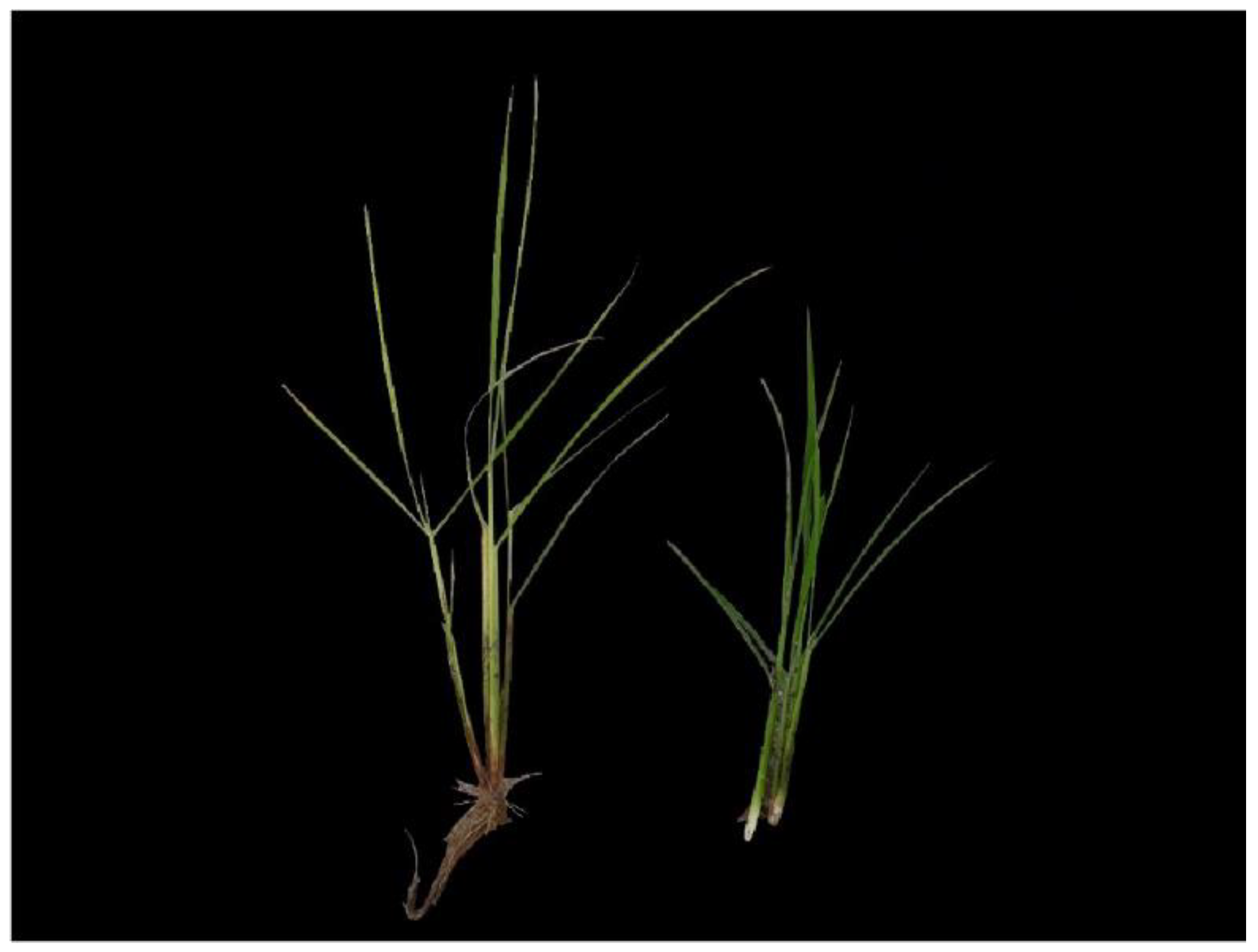
Figure 1.
Rice infected with Bakanae disease (left) and normal rice (right).
Figure 1.
Rice infected with Bakanae disease (left) and normal rice (right).
Figure 2.
The rice infected with Bakanae disease photographed from above (Red box corresponds to RBD-infected bunch).
Figure 2.
The rice infected with Bakanae disease photographed from above (Red box corresponds to RBD-infected bunch).
Figure 3.
The standardized rice transfer interval due to agricultural mechanization.
Figure 3.
The standardized rice transfer interval due to agricultural mechanization.
Figure 4.
Example bunch and culm of rice plant.
Figure 4.
Example bunch and culm of rice plant.
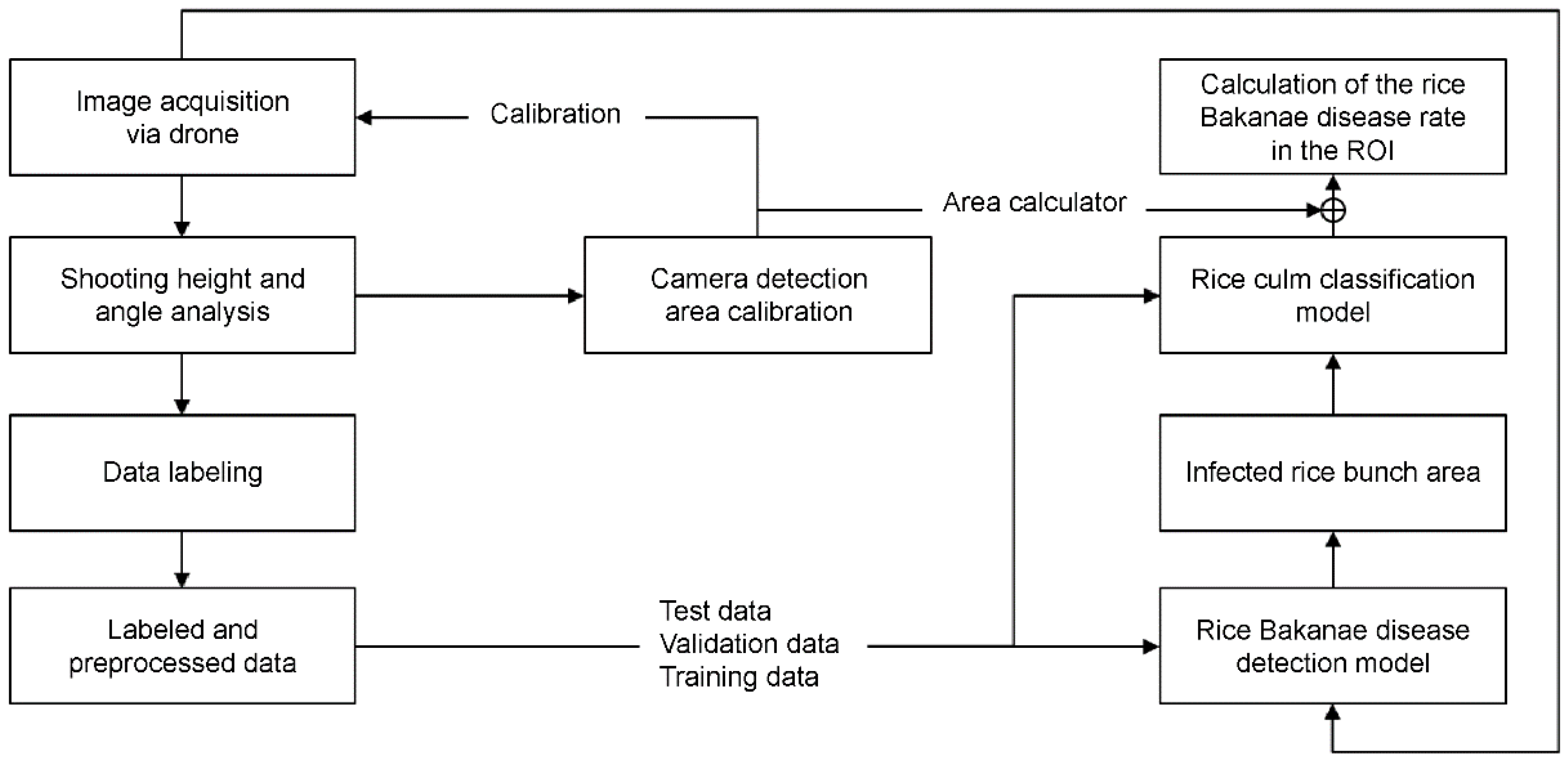
Figure 5.
The system structure for reading the RBD-infected.
Figure 5.
The system structure for reading the RBD-infected.
Figure 6.
The algorithm flowchart for calculating RBD recognition degree.
Figure 6.
The algorithm flowchart for calculating RBD recognition degree.
Figure 7.
An example of image cropping RBD and normal rice plants: (a) Images in which the area containing rice infected with Bakanae disease is cropped, and (b) images in which an area containing normal rice is cropped.
Figure 7.
An example of image cropping RBD and normal rice plants: (a) Images in which the area containing rice infected with Bakanae disease is cropped, and (b) images in which an area containing normal rice is cropped.
Figure 8.
The edge detection of images containing RBD: (a) Original image, and (b) edge image containing gradient magnitude values.
Figure 8.
The edge detection of images containing RBD: (a) Original image, and (b) edge image containing gradient magnitude values.
Figure 9.
The process of determining the number of RBD-infected culms.
Figure 9.
The process of determining the number of RBD-infected culms.
Figure 10.
The method of creating patch image data using sliding window.
Figure 10.
The method of creating patch image data using sliding window.
Figure 11.
Calculation of the camera field of view for the operating drone.
Figure 11.
Calculation of the camera field of view for the operating drone.
Figure 12.
Drone images collected from various height and angles conditions (A–D) heights of 1, 2, 3, and 4 m, respectively; (1–4) 0°, 10°, 20°, and 30° down angles, respectively.
Figure 12.
Drone images collected from various height and angles conditions (A–D) heights of 1, 2, 3, and 4 m, respectively; (1–4) 0°, 10°, 20°, and 30° down angles, respectively.
Figure 13.
Random cropping procedure from original image.
Figure 13.
Random cropping procedure from original image.
Figure 14.
Example of data by number of culms of RBD (The numbers in the upper left mean the actual number of culm).
Figure 14.
Example of data by number of culms of RBD (The numbers in the upper left mean the actual number of culm).
Figure 15.
The rest results of recognition degree for RBD based on the selection of shooting height and angle (The red box indicates the height and angle at which the mean of the gradient magnitude, hue, and saturation LDA is the highest).
Figure 15.
The rest results of recognition degree for RBD based on the selection of shooting height and angle (The red box indicates the height and angle at which the mean of the gradient magnitude, hue, and saturation LDA is the highest).
Figure 16.
Visualization of LDA results by shooting conditions (The red box indicates the height and angle at which the mean of the gradient magnitude, hue, and saturation LDA is the highest).
Figure 16.
Visualization of LDA results by shooting conditions (The red box indicates the height and angle at which the mean of the gradient magnitude, hue, and saturation LDA is the highest).
Figure 17.
The images taken for camera calibration.
Figure 17.
The images taken for camera calibration.
Figure 18.
The perspective transformation for camera calibration: (A) reference lines and points for performing perspective transformations, (B) image projection from pixel coordinate to world coordinate, (C) center compensation based on the camera center point, (D) calculated recognition range using camera calibration.
Figure 19.
The detection results of RBD bunch area for patch segmentation data (Red boxes represent detected RBD-infected bunches): (A) warm up and label smoothing technique not applied, and (B) warmup and label smoothing techniques applied.
Figure 19.
The detection results of RBD bunch area for patch segmentation data (Red boxes represent detected RBD-infected bunches): (A) warm up and label smoothing technique not applied, and (B) warmup and label smoothing techniques applied.
Figure 20.
YOLOv3 model-based RBD bunch area detection results (Yellow boxes represent the ground truths, and red boxes represent the detection results): (A–C) Each detection task, (1) Ground truth, and (2) predicted result.
Figure 20.
YOLOv3 model-based RBD bunch area detection results (Yellow boxes represent the ground truths, and red boxes represent the detection results): (A–C) Each detection task, (1) Ground truth, and (2) predicted result.
Figure 21.
The prediction result of RBD for 50 layers of deep residual network.
Figure 21.
The prediction result of RBD for 50 layers of deep residual network.
Figure 22.
The prediction result of RBD based on reconstructed number of culms data.
Figure 22.
The prediction result of RBD based on reconstructed number of culms data.
Figure 23.
The comparison of classification performance for RBD infected culm data.
Figure 23.
The comparison of classification performance for RBD infected culm data.
Table 1.
A comparison of object detection models based on Pascal VOC 2007 dataset.
Table 1.
A comparison of object detection models based on Pascal VOC 2007 dataset.
| Model | mAP | FPS |
|---|
| Faster R-CNN (ResNetV2 101) [23] | 74.63 | 7 |
| FPN (ResNetV2 101) [24,25] | 75.89 | 6 |
| Bi-FPN (ResNetV2 101) [26,27] | 76.04 | 23 |
| YOLOv2 (DarkNet 53) [28] | 78.60 | 41 |
| YOLOv3 (DarkNet 53) [29] | 80.15 | 36 |
Table 2.
The data collected to select the drone’s shooting height and angle.
Table 2.
The data collected to select the drone’s shooting height and angle.
| Taking Height (m) | Taking Downward Angle (°) | Total |
|---|
| 0 | 5 | 10 | 15 |
|---|
| 1 | 126 | 126 | 128 | 126 | 506 |
| 2 | 126 | 126 | 128 | 126 | 506 |
| 3 | 126 | 124 | 126 | 127 | 503 |
| 4 | 126 | 124 | 125 | 124 | 499 |
| Total | 504 | 500 | 507 | 503 | 2014 |
Table 3.
The number of data collected for the training detection and classification model.
Table 3.
The number of data collected for the training detection and classification model.
| Collection Period | Area | Number of Images |
|---|
| 7/2020~8/2020 | Jeolla-do | 100 |
| 7/2021~8/2021 | Jeolla-do | 7548 |
| Gyeongsang-do | 11,095 |
| Chungcheong-do | 1771 |
| Total | 20,514 |
Table 4.
The data for classification of RBD infected culms.
Table 4.
The data for classification of RBD infected culms.
| Number of RBD Infected Culms | Train | Validation | Test | Total |
|---|
| 1 | 3258 | 838 | 94 | 4190 |
| 2 | 7087 | 1839 | 180 | 9106 |
| 3 | 7655 | 1870 | 176 | 9701 |
| 4 | 5252 | 1265 | 112 | 6629 |
| 5 | 1282 | 326 | 70 | 1678 |
| 6 | 281 | 71 | 20 | 372 |
| 7 | 92 | 18 | 17 | 127 |
| 8 | 16 | 2 | 5 | 23 |
| Total | 24,923 | 6229 | 674 | 31,826 |
Table 5.
YOLOv3 model training parameters.
Table 5.
YOLOv3 model training parameters.
| Parameter Name | Parameter Value |
|---|
| Batch size | 5 |
| Total epochs | 120 |
| Batch normalization | True |
| Batch normalization decay | 0.99 |
| Weight decay | 5 × |
| Learning rate | 1 × |
| Cosine learning rate decay | True |
| Non-maximum suppression threshold | 0.45 |
| Pre-train weight | ImageNet |
Table 6.
YOLOv3 model performance results for culm area detection of RBD.
Table 6.
YOLOv3 model performance results for culm area detection of RBD.
| Network | Warm Up | Label Smoothing | mAP |
|---|
| Train | Validation | Test |
|---|
| DarkNet53 | False | False | 95.09% | 80.75% | 81.33% |
| False | True | 95.28% | 91.36% | 89.22% |
| True | False | 91.64% | 89.95% | 88.13% |
| True | True | 97.84% | 92.68% | 90.49% |
Table 7.
The deep residual network training parameters.
Table 7.
The deep residual network training parameters.
| Parameter | Method |
|---|
| Image size | 224 × 224 × 3 |
| Batch size | 16 |
| Total epochs | 300 |
| Learning rate | 0.001 |
| Weight decay | 0.00004 |
| Batch normalization | True |
| Optimizer | Adam |
| Loss function | Focal loss (= 4.0, = 2.0) |
| Weight initialization | Xavier initialization |
| Pre-train weight | ImageNet |
| Network | ResNetV2(50/101/152) |
Table 8.
The comparison of culm classification performance by deep residual network depth.
Table 8.
The comparison of culm classification performance by deep residual network depth.
| Depth | 50 Layers | 101 Layers | 152 Layers |
|---|
| Accuracy | 80.36% | 70.45% | 75.95% |
Table 9.
The number of culm classification performance results for 50 layers of deep residual network.
Table 9.
The number of culm classification performance results for 50 layers of deep residual network.
| Number of RBD Infected Culms | Test | True (Pred) | False (Pred) | Accuracy |
|---|
| 1 | 94 | 89 | 5 | 94.68% |
| 2 | 180 | 168 | 12 | 93.33% |
| 3 | 176 | 154 | 22 | 87.50% |
| 4 | 112 | 99 | 13 | 88.39% |
| 5 | 70 | 59 | 11 | 84.28% |
| 6 | 20 | 14 | 6 | 70.00% |
| 7 | 17 | 11 | 6 | 64.70% |
| 8 | 5 | 3 | 2 | 60.00% |
| Total | 674 | 597 | 77 | 80.36% |
Table 10.
The reconstructed number of RBD infected culm classification training and evaluation datasets.
Table 10.
The reconstructed number of RBD infected culm classification training and evaluation datasets.
| Number of RBD Infected Culms | Original | Train | Validation | Test |
|---|
| 1 | 4190 | 3258 | 838 | 94 |
| 2 | 9106 | 7087 | 1839 | 180 |
| 3 | 9701 | 7655 | 1870 | 176 |
| 4 | 6629 | 5252 | 1265 | 112 |
| 5 | 1678 | 1282 | 326 | 70 |
| Total | 31,304 | 24,534 | 6139 | 632 |
Table 11.
The comparison of culm classification performance by deep residual network depth.
Table 11.
The comparison of culm classification performance by deep residual network depth.
| Depth | 50 Layers | 101 Layers | 152 Layers |
|---|
| Accuracy | 81.72% | 85.36% | 84.44% |
Table 12.
Culm number classification performance results for deep residual network 101.
Table 12.
Culm number classification performance results for deep residual network 101.
| Number of RBD Infected Culms | Test | True (Pred) | False (Pred) | Accuracy |
|---|
| 1 | 94 | 85 | 9 | 90.42% |
| 2 | 180 | 152 | 28 | 84.44% |
| 3 | 176 | 153 | 23 | 86.93% |
| 4 | 112 | 92 | 20 | 82.14% |
| 5 | 70 | 58 | 12 | 82.85% |
| Total | 632 | 540 | 92 | 85.36% |


