Validation of Soil Survey Estimates of Saturated Hydraulic Conductivity in Major Soils of Puerto Rico

Abstract

Ranges or “classes” of probable saturated hydraulic conductivity values (K_sat) are listed for all soil series in USDA-NRCS Soil Survey reports. Listed values are not measured, but rather estimated from other soil properties using a pedotransfer function (PTF). To validate the PTF, we compared estimated K_sat classes with measured values in various horizons of nine major soil series of Puerto Rico. For each horizon, a minimum of 9 and usually 16 K_sat measurements were made with Guelph permeameters near locations where soil pedons had been thoroughly described. In most horizons, K_sat was log-normally distributed. The ratios of K_sat values corresponding to one geometric standard deviation above and below the mean were usually less than 10, which is the ratio of upper and lower class boundaries in the K_sat classification system. For most horizons, measured K_sat values were distributed among the rated K_sat class and the next higher class, indicating that the PTF systematically underestimated the K_sat distributions, but by less than an order of magnitude. From the point of view of soil and water management decisions requiring conservative K_sat estimates, the PTF estimates appeared reasonably conservative without deviating from actual values so as to limit the usefulness of the estimates.

1. Introduction

One of the fundamental physical properties of soil is its saturated hydraulic conductivity (K_sat), defined as the rate of water movement through saturated soil under a unit hydraulic gradient. Knowledge of K_sat is essential for predicting the magnitude of environmental processes such as water infiltration, runoff, and soil erosion, and for designing irrigation, drainage, and land-applied waste disposal systems [1,2,3,4,5]. Engineering properties of soil, such as consolidation rate, fluidization, piping, and embankment stability, are strongly influenced by the capacity of water to move through the soil, and, hence, by K_sat [6,7]. For these reasons, information on K_sat is a standard component of Soil Survey reports.

Field and laboratory determinations of K_sat are expensive and time consuming, and require large numbers of measurements in order to account for high coefficients of variability which can exceed 400 percent [8]. The variability is compounded when K_sat measurements are separated by large spatial distances [8,9,10], or taken at different times [11,12]. This has led to estimates of K_sat based on pedotransfer functions (PTFs), which estimate values from correlated soil properties that are readily available in Soil Survey reports, such as texture, bulk density, organic matter, particle size distribution, and structure descriptions. Early evidence of the usefulness of PTFs for estimating K_sat came from the work of O’Neal [13,14], who developed a set of field clues for estimating K_sat. He found good agreement between measured and estimated K_sat values in 68 percent of a total of 271 soil horizons examined. To account for intrinsic soil variability, he assigned each of the soil horizons to one of seven “percolation classes” defined by ranges of probable K_sat values, rather than assigning a single average value to each horizon. A similar “class” approach for estimating K_sat in soils based on field textural and structural observations was adopted by McKeague et al. [15], who observed that 87 percent of estimated K_sat values from 78 soil horizons deviated from measured values by one K_sat class or less. Beginning with such seminal works, an enormous body of literature on PTF methodology has flourished [16,17,18,19,20,21]. These vary in complexity, from simple class systems to highly complex schemes based on neural networks.

One of the simplest yet most widely used PTFs for estimating K_sat in the continental USA and its territories is described in Section 618 of the National Soil SurveyHandbook published by the USDA-NRCS [22]. The structure of the PTF is similar to that outlined by Pachepsky and Park [23]. Soils are separated into groups based on their location in the classical USDA textural triangle and bulk density groups defined broadly as “high”, “medium” and “low”. Depending on soil location in the textural triangle and bulk density grouping, soils are assigned to classes of probable K_sat values, each varying over an order of magnitude. A list of auxiliary or overriding criteria, consisting primarily of soil structural descriptions, is also provided. Whenever one of the overriding criteria is encountered, a K_sat class specific to that overriding criterion is assigned regardless of soil texture and bulk density. Estimates of K_sat class based on this PTF are available for all soil series of the US, including Puerto Rico, and are listed in the NRCS National Soil Information System (NASIS) database. The different classes are defined in

Table 1. Soil saturated hydraulic conductivity classes (Soil Survey Staff [22]).

Saturated Hydraulic Conductivity Range (µm/s)	Range of Log Ksat Values	Description of Saturated Hydraulic Conductivity Class
<0.01	<−2	Very low
0.01–0.1	−1 to −2	Low
0.1–1.0	0 to −1	Moderately low
1.0–10	0 to 1	Moderately high
10–100	1 to 2	High
>100	>2	Very high

.

Published studies are available comparing predictions of large numbers of PTF models to data sets of thousands of field and laboratory K_sat measurements [17,18,19,20,21,22,23]. However, in surveying this literature, it is difficult to find studies evaluating the specific USDA-NRCS pedotransfer function described above. Pachepski and Park [23] compared a similar model based on texture and bulk density to several thousand K_sat measurements in the USA. They found that the predictive accuracy of the PTF was not high, and yet was comparable with estimates obtained from far more detailed soil information using sophisticated machine learning methods.

Gupta et al. [21] assembled a global database of soil saturated hydraulic conductivity (SoilKsatDB) involving 13,267 K_sat measurements from 1910 sites for use in PTF modeling. They commented that PTFs derived for soils in temperate soils may not be suitable for estimating K_sat in tropical regions. This is of particular relevance to K_sat estimates in Puerto Rico and other tropical islands of the Caribbean basin, which are based on PTF models developed primarily in temperate regions.

The objective of this research was to validate K_sat estimates based on the USDA-NRCS pedotransfer function for major soils of Puerto Rico occupying large land areas and holding key positions in the soil classification system. The estimates are listed in NASIS databases for these soils. Validation was achieved by comparing estimated K_sat classes with multiple measured values in the same soils.

2. Materials and Methods

2.1. Description of the Project Area

Saturated hydraulic conductivity was measured in situ in various horizons from 9 soil series of Puerto Rico, which had previously been thoroughly characterized by NRCS Soil Survey personnel. The soil series and their classifications according to the USDA Soil Taxonomy system are given in

Table 2. Soil series included in the study.

Soil Series	Classification according to USDA Soil Taxonomy and Approximate WRB Reference Soil Group
Aceitunas	Fine, kaolinitic, isohyperthermic Typic Paleudults WRB reference soil group: Alisols
Bahía	Mixed, kaolinitic, isohyperthermic Typic Paleargids WRB reference soil group: Planosols
Bayamón	Very-fine, kaolinitic, isohyperthermic Typic Hapludox WRB reference soil group Ferrasols
Coto	Very-fine, kaolinitic, isohyperthermic Typic Eutrustox WRB reference soil group Ferrasols
Descalabrado	Clayey, mixed, superactive, isohyperthermic, shallow Typic Haplustolls WRB reference soil group: Kastonozem
Fraternidad	Fine, smectitic, isohyperthermicTypic Haplusterts WRB reference soil group: Vertisols
Humatas	Very-fine, parasesquic, isohyperthermic Typic Haplohumults WRB reference soil group: Alisols
Nipe	Very-fine, ferruginous, isohyperthermic Anionic Acrudox WRB reference soil group: Ferrasols
Pandura	Coarse-loamy, mixed, active, isohyperthermic, shallow Dystric Eutrudepts WRB reference soil group Cambisols
Toa	Fine, mixed, active, isohyperthermic Fluvaquentic Hapludolls WRB reference soil group Phaeozems

, together with the approximate Reference Soil Group in the World Reference Base (WRB) system [24].

The K_sat measurement sites for each soil series were located as close as possible to pedons which had previously been characterized by Soil Survey personnel. The geographic locations and USDA-NRCS Pedon Identification Numbers of these pedons are given in

Table 3. Coordinates of soil pedons nearest K_sat measurement sites.

Soil Series	Pedon ID	Latitude	Longitude
Aceitunas	S09PR005-001	18°26′04″ N	67°07′06.8″ W
Bahía	S81PR007-001	17°58′12.0″ N	67°11′43.0″ W
Bayamón	S63PR143-001	18°25′48″ N	66°18′15″ W
Coto	S82PR071-001	18°27′53″ N	67°03′19″ W
Descalabrado	S61PR121-002	18°02′39″ N	66°59′00″ W
Fraternidad	S61PR079-001	18°00′58.0″ N	67°04′26.0″ W
Humatas	S94PR097-001	18°12′40″ N	67°08′00″ W
Nipe	S57PR097-001	18°11′11.0″ N	67°06′35.0″ W
Pandura	S09PR129-001	18°07′17.2″ N	65°57′35.8″ W
Toa	S63PR067-001	18°07′32.0″ N	67°06′36.0″ W

, and a corresponding map is given in Figure 1. To minimize temporal effects on K_sat, the measurements were made in pasture lands that had been undisturbed for several years prior to sampling. All measurements at a given site were made on the same day.

2.2. Experimental Techniques

At each site, the usual procedure was to set up a 4 × 4 sampling grid (for a total of n = 16 grid points), with a distance between grid points of approximately 6 m. The only exceptions were the sampling site for the Pandura series, where a 3 × 4 sampling grid was used, and the Bahia site, with a 3 × 3 sampling grid. A relatively close 6 m spacing between K_sat measurements at each site was used in order to capture intrinsic (random) soil variability near the pedon and minimize spatially correlated variations. At each grid point, K_sat was measured in situ using variants of the Guelph permeameter method [25,26], with the specific variant depending on whether K_sat was measured in surface or subsurface horizons.

For measurements in surface horizons, the top 2 cm of soil was removed to eliminate vegetation and debris. Sharpened PVC or stainless steel cylinders 10 cm long and of 10 cm interior diameter were driven into the ground to a depth (d) of 4 cm (Figure 2). Soil immediately in contact with the inner and outer sides of the cylinder was pressed against the sides with a sharp stick to eliminate air gaps between the soil and cylinder walls. Ponded water at constant head (H) was then established inside the cylinders using a Guelph permeameter (Soilmoisture Equipment Corp., Santa Barbara, CA, USA), and the volumetric outflow rate (q) $\left(\mathrm{volume}/\mathrm{time}\right)$ from the permeameter was measured once steady state infiltration was reached, usually within 30–60 min.

Hydraulic conductivity K_sat was calculated from the formula [16]:

$$K_{sat}=\frac{Gq}{\left[a\left(H+\lambda \right)+G\pi a^2\right]}$$

(1)

where the parameter G is a shape factor given by

$$G=0.36\frac{d}{a}+0.184$$

(2)

and the cylinder configuration parameters a, d and H are defined in Figure 2. The parameter $\lambda$ in Equation (1) with dimensions of length (cm), is the exponent in the hydraulic conductivity function

$$K\left(h\right)=K_{sat}\exp \left(-\frac{h}{\lambda }\right)$$

(3)

where h (cm) is the suction head and K (h) is the soil hydraulic conductivity corresponding to h. The parameter $\lambda$ has been used as a flow-weighted wetting front suction head in Green–Ampt infiltration models [25].

Estimates of $\lambda$ for different texture/structural classes are described in

Table 4. Texture–Structure categories for visual estimation of λ. Adapted from Elrick et al. [25].

Texture–Structure Category	λ * (cm)
Compacted, structureless, clayey, or silty materials such as landfill caps and liners, lacustrine or marine sediments, etc.	100
Most structured and medium textured materials; include structured clayey and loamy soils, as well as unstructured medium sands. This category is generally the most appropriate for agricultural soils.	25
Soils that are both fine textured and massive; include unstructured clayey and silty soils, as well as structureless sandy materials.	8
Coarse and gravelly sands; may also include some highly structured soils with large numerous cracks and biopores.	3

* The parameter $\lambda$ in Table 9 and Equations (1), (3) and (4) is the inverse of another parameter (α) which was used by Reynolds et al. [25,26] in their description of Guelph permeameter theory. Our preference for using $\lambda$ rather than α stems from the clear physical meaning of the former as a flow-weighted wetting front suction head in the Green–Ampt infiltration model [25].

. As all soils in this study were reasonably well structured, the parameter value $\lambda =8 \mathrm{cm}$ was assumed. Although $\lambda$ is estimated rather than directly measured, the resulting error in K_sat estimates is usually small, within a factor of 2 of the actual value [25,26]. This uncertainty is small compared to within field variations of K_sat, which can vary over 1 to 2 orders of magnitude.

For measuring K_sat in subsurface horizons, a cylindrical hole of radius a = 5 cm was bored to the desired depth where K_sat was to be measured. The bottom of the hole was flattened with a planing auger. To minimize soil smearing effects on K_sat measurements, augering of very wet soils was avoided, and the walls of the auger hole were cleaned with a stiff brush which partially removed any smear layer. The permeameter tip was placed in the hole and water was allowed to infiltrate the soil until a steady state was reached under a constant water head (H) which was normally 5 cm, and 10 cm in very impermeable soils. The system is illustrated in Figure 3.

The hydraulic conductivity K_sat was calculated from the measured steady state flux q as [26]:

$$K_{sat}=\frac{Cq}{\left[\left(\frac{2\pi H^2 + C\pi a^2}{\lambda }\right)+2\pi H\right]}$$

(4)

where C is a constant shape factor [25] that is dependent on $\lambda$ and the ratio $H/a$. In our measurements, the well radius a was 3 cm and the hydraulic head H was either 5 or 10 cm.

The Guelph permeameter method was chosen as it is a theoretically well-founded field method that allows measuring K_sat in situ using relatively small amounts of water. A requirement is that a steady state water infiltration (q) must be achieved prior to measurement, but in most cases this is achieved within 30–60 min of infiltration. As illustrated in Figure 2 and Figure 3, the infiltrating water is confined to a relatively small bulb-shaped wetting zone in the soil, which allows good depth resolution of K_sat measurements. The method can be applied using either one or two values of hydraulic head (H). In the single-head method, the infiltration rate (q) is measured at a given head (H) and the wetting front suction parameter $\lambda$ is estimated from Table 4. This method typically gives a measurement accuracy of $0.5K_{sat}\le X\le 2K_{sat}$, where X is the measured value and K_sat is the true saturated conductivity value [24]. In the two-head method, the infiltration rate (q) is measured at two different infiltrometer heads (H), which allows the measurement of both K_sat and $\lambda$, and typically gives more accurate values of K_sat. However, this method consumes twice the amount of water and time as the single-head technique, and is mathematically ill-conditioned, which can cause unreasonable estimates of K_sat and $\lambda$ [24,25]. Since our study involved large numbers of measurements to be completed in a single day at any given field site, requiring hand-carrying of all the necessary water, practical considerations dictated that the single-head method was preferable.

3. Results

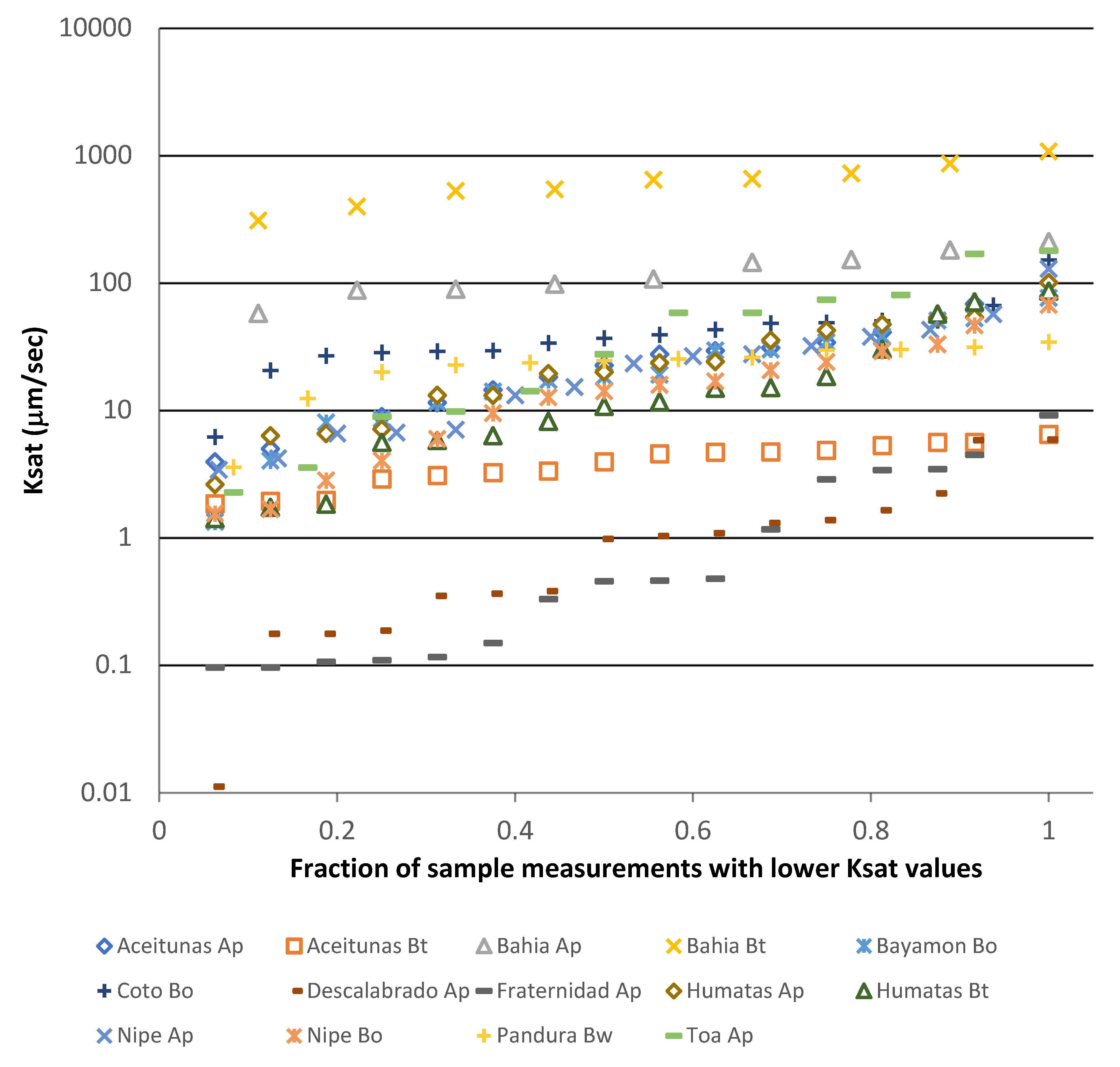
Cumulative distributions of measured K_sat values in the different soil horizons are shown in Figure 4. Shapiro–Wilks tests on the distributions showed that they were nearly all log-normally distributed. Consequently, all subsequent parametric statistical tests were performed on log-transformed K_sat values.

For such distributions, the arithmetic mean $\overline{\log K}$ from a sample of n = 1, 2, …, N values of log K_sat values is given by

$$\overline{\log K}=\frac{1}{N}{\displaystyle \sum }_{n=1}^N\log K_{sat}=\log {\overline{K}}_{geo}$$

(5)

where ${\overline{K}}_{geo}$ is the geometric mean defined by

$${\overline{K}}_{geo}\equiv {\left({\displaystyle \prod }_{n=1}^N{\left(K_{sat}\right)}_n\right)}^{\frac{1}{N}}$$

(6)

The standard deviation of log K_sat values, ${\sigma }_{\log K}$ is defined by

$${\sigma }_{\log K}\equiv \log K_{83.5}-\log K_{50}=\log K_{50}-\log K_{16.5}=\log {\sigma }_{geo}$$

(7)

where ${\sigma }_{geo}$ is the geometric standard deviation, defined by

$${\sigma }_{geo}\equiv \frac{K_{83.5}}{K_{50}}=\frac{K_{50}}{K_{16.5}}$$

(8)

The parameters $K_{16.5}$, $K_{50}$ and $K_{83.5}$ are K_sat values corresponding to the cumulative distribution percentiles 16.5, 50, and 83.5, respectively. The parameters $K_{83.5}$ and $K_{16.5}$ constitute the upper and lower bounds of the middle 67 percent of all K_sat values, i.e., the percent of values residing within one geometric standard deviation of the geometric mean.

Table 5. Statistical data for K_sat values measured in different soil horizons.

Soil Horizon	Group 1	N2	Rated Ksat Class (μm/s)	$$\begin{gathered} {\overline{\mathit{K}}}_{\mathit{g}\mathit{e}\mathit{o}} \\ (\mathsf{\mu }\mathbf{m}/\mathbf{s}) \end{gathered}$$	${\mathit{\sigma }}_{\mathit{g}\mathit{e}\mathit{o}}$	$$\begin{gathered} {\mathit{K}}_{16.5} \\ (\mathsf{\mu }\mathbf{m}/\mathbf{s}) \end{gathered}$$	$$\begin{gathered} {\mathit{K}}_{83.5} \\ (\mathsf{\mu }\mathbf{m}/\mathbf{s}) \end{gathered}$$	$\frac{{\mathit{K}}_{83.5}}{{\mathit{K}}_{16.5}}$
Bahia Bt	a	9	10–100	591.56	1.46	404.58	864.97	2.14
Bahia Ap	ab	9	10–100	117.95	1.51	77.62	176.2	2.27
Coto Bo	bc	16	1–10	36.73	1.94	18.97	71.12	3.75
Toa Ap	c	12	1–10	27.35	4.27	6.41	116.68	18.2
Pandura Bw	c	12	10–100	21.09	1.86	11.35	39.17	3.45
Aceituna Ap	c	16	1–10	20.18	2.48	8.13	50.12	6.16
Humatas Ap	c	16	0.1–1	19.86	2.67	7.45	52.97	7.11
Bayamon Bo	c	16	1–10	17.41	2.83	6.15	49.32	8.02
Nipe Ap	c	16	1–10	17.17	2.75	6.24	47.1	7.64
Nipe Bo	cd	16	1–10	11.67	3.13	3.73	36.48	9.78
Humatas Bt	cd	16	0.1–1	10.96	3.52	3.11	38.64	12.42
Aceituna Bt	d	16	1–10	3.74	1.49	2.51	5.58	2.22
Descalabrado Ap	e	16	0.1–1	0.64	4.81	0.13	3.07	23.62
Fraternidad Ap	e	16	0.1–1	0.57	4.86	0.12	2.77	23.08

¹ Statistical difference according to ANOVA and Tukey test. ² Number of K_sat measurements for the corresponding horizon.

lists the soil horizons evaluated, the number N of K_sat measurements per horizon, the rated K_sat class in the USDA-NRCS system, the measured geometric mean of K_sat, the geometric standard deviation, the respective upper and lower geometric standard deviation bounds $K_{83.5}$ and $K_{16.5}$, and the ratios $\frac{K_{83.5}}{K_{16.5}}$.

Statistical differences among the means of the distributions are indicated by the lower case letters in the second column. Soil horizon names followed by a given letter in common are not statistically different at the p < 0.05 level. Statistical differences were determined by performing ANOVA and Tukey tests on the log transformed K_sat values. Each sampled soil horizon was considered a different experimental treatment, and the number of K_sat measurements for that horizon were taken as the corresponding number of replications. Results show that 9 of the 14 soil horizons are not statistically different from one another. The two sandy Bahía soil horizons had K_sat values significantly higher than all other soil series except Coto, a clayey Oxisol. The two soils with statistically lower K_sat values than all others were Descalabrado and Fraternidad, both characterized by abundance of 2:1 clay minerals.

Inspection of the right hand columns of Table 5 shows that the ratios of K_sat values corresponding to one geometric standard deviation above and below the mean, i.e., $K_{83.5}/K_{16.5}$, were usually less than 10, which is the ratio of upper and lower class boundaries in the K_sat classification system. This means that, in most cases, the assigned class bandwidth of an order of magnitude was sufficient to capture most of the variability of K_sat values in a given sample. The two most important exceptions occurred in the case of the two soils with lowest K_sat values, Fraternidad and Descalabrado, characterized by abundance of 2:1 clay minerals. In this case, the ratio $K_{83.5}/K_{16.5}$ was approximately 20, indicating a considerably broader distribution than that assumed in the rating system. Inspection of Table 5 and Figure 5 shows a reasonably strong inverse relation between the dispersion parameter $K_{83.5}/K_{16.5}$ and the geometric mean ${\overline{K}}_{geo}$.

However, although the measured K_sat distributions were of comparable dispersion as the rated class boundaries, the measured K_sat distributions were always shifted upwards relative to the rated K_sat class, indicating that the PTF systematically underpredicted the actual values. This can be seen in

Table 6. Fraction of measured K_sat values in expected classes, and in one or two classes higher or lower than the expected class.

Soil Series	Expected	Higher Ksat by		Lower Ksat by
	Ksat Category	One Category	Two Categories	One Category	Two Categories
Aceituna Ap	0.25	0.75	-	-	-
Aceituna Bt	1.00	-	-	-	-
Bahia Ap	0.22	0.78	-	-	-
Bahia Bt	0.89	0.11	-	-	-
Bayamon Bo	0.25	0.75	-	-	-
Coto Bo	0.82	0.06	0.06	0.06	-
Descalabrado Ap	0.50	0.50	-	-	-
Fraternidad Ap	0.50	0.38	0.13	-	-
HumatasAp	0.06	0.25	0.69	-	-
HumatasBt	0.00	0.44	0.56	-	-
Nipe Ap	0.38	0.56	-	0.06	-
Nipe Bo	0.38	0.62	-	-	-
Pandura Bw	0.92	0.08	-	-	-
Toa Ap	0.33	0.50	0.17	-	-

, which gives the fraction of measured K_sat values occurring within the expected (rated) class, and the fractions occurring in classes one or two orders of magnitude higher or lower than the expected class. For all soils, the bulk of measured K_sat values occurred either in the rated class or in classes above it, with almost no measured values occurring below the rated class. For most soils, 90 percent or more of the K_sat data were distributed among the rated class and the class immediately above it, indicating that the PTF underpredicted the actual K_sat values by no more than one class or one order of magnitude. A significant exception occurred in the case of the two Humatas horizons, for which the PTF placed the rated class (0.1–1 ${\mathsf{\mu }\mathrm{m}\mathrm{s}}^{-1}$) one or two orders of magnitude below the actual K_sat values.

4. Discussion

The above results confirm the need to assign a wide range in K_sat values to a given class, as is currently recognized in the USDA-NRCS pedotransfer function. The measured dispersion of K_sat values around the geometric mean was usually comparable to the 10-fold dispersion implicit in the pedotransfer function, except in the case of soils with very low K_sat values (soils with abundance of expandible 2:1 clay minerals) where a broader dispersion of values was observed. Other authors [27,28] have encountered spreads in K_sat values commonly within ranges of one or two orders of magnitude.

For the most part, the USDA-NRCS pedotransfer function tended to underestimate K_sat values, as indicated by the fact that most experimental values occurred either in the rated K_sat class or in the class immediately above it. This result is similar to that of Sobieraj et al. [17], who compared K_sat estimates of nine PTF models to measured values in a tropical watershed, and noticed that in the 0–0.1 soil depth interval, all PTF models slightly underestimated the K_sat values. In our study, the difference between estimated and measured K_sat values was usually no greater than one K_sat class, comparable to the results of McKeague et al. [15] in soils from Canada and northeastern USA, and findings in the pioneering study by O’Neil [13,14] in soils from the USA.

This study only considered spatial variation of K_sat measurements over short distances. To minimize the possibility of significant temporal effects, all measurements were performed in soil horizons that were under pasturewhich, other than grazing, had not been disturbed for at least three or four years. Kargas et al. [28] noted from their own work and other cited research that temporal variability of K_sat can be small in soils covered by the same vegetation throughout the year and subject to no recent human intervention.

From the point of view of soil and water management decisions based on estimated K_sat classes, it is often safer to underestimate K_sat than to overestimate it. For example, in the case of land application of waste water or liquid manure, an underestimate of K_sat will ensure that the recommended rate of source application (based on K_sat) will not overload the infiltration capacity of the soil, thereby reducing the risk of runoff and negative environmental impact. On the other hand, it is desirable that the estimated K_sat class not be too far below the actual class, which would lead to an economically under-designed system. For most soil horizon in this study, the USDA-NRCS estimation system appeared to satisfy these criteria by systematically underpredicting actual K_sat values by a margin not exceeding one order of magnitude. The single exception to this observation was the Humatas soil, for which the rating system underpredicted K_sat by one or two orders of magnitude.

We believe that the rather severe underprediction of K_sat for the Humatas series, a dominant Ultisol in Puerto Rico, was probably due to over-weighting of texture and bulk density effects in the PTF, and not enough weighting of micro-structure effects associated with highly weathered clay minerals in Ultisols. Our suggestion is that for all Oxisols and Ultisols, which are highly weathered by definition, a K_sat class of at least 1–10 ${\mathsf{\mu }\mathrm{m}\mathrm{s}}^{-1}$ should be assigned by default. This would be consistent with our results presented here, and also with a classic study by Lugo-Lopez et al. [29], where eighth hour infiltration rates measured with ring infiltrometers in Oxisols and Ultisols of Puerto Rico always exceeded 0.8 in h${\mathrm{r}}^{-1}$ or 5.7 ${\mathsf{\mu }\mathrm{m}\mathrm{s}}^{-1}$.

References

- Lane, L.J.; Nearing, M.A. (Eds.) USDA-Water Erosion Prediction Project: Hillslope Profile Model Documentation; NSERL Report No. 2; USDA-ARS National Soil Erosion Research Laboratory: West Lafayette, IN, USA, 1989. [Google Scholar]
- Hillel, D. Environmental Soil Physics; Elsevier: Amsterdam, The Netherlands, 1998. [Google Scholar]
- Sharma, V. Fundamentals of Soil and Water Conservation Engineering; Academic Publications: Rohini, India, 2019. [Google Scholar]
- Soil Survey Staff. National Engineering Handbook, 2nd ed.; USDA-NRCS: Washington, DC, USA, 1991. [Google Scholar]
- Soil Survey Staff. National Handbook for Conservation Practices; 450-NHCP; USDA-NRCS: Washington, DC, USA, 2019. [Google Scholar]
- Mitchell, D. Fundamentals of Soil Behavior; Wiley: Hoboken, NJ, USA, 2005. [Google Scholar]
- Das, B.M.; Sobhan, K. Principles of Geotechnical Engineering; Cengage: Stamford, CT, USA, 2014. [Google Scholar]
- Warrick, A.W.; Nielsen, D.R. Spatial variability of soil physical properties in the field. In Applications of Soil Physics; Hilell, D., Ed.; Academic Press: Toronto, ON, Canada, 1980; pp. 319–344. [Google Scholar]
- Warrick, A.W. Spatial variability. In Environmental Soil Physics; Hillel, D., Ed.; Academic Press: New York, NY, USA, 1998. [Google Scholar]
- Gupta, N.; Rudra, R.P.; Parkin, G. Analysis of spatial variability of hydraulic conductivity at field scale. Can. Biosyst. Eng. 2006, 48, 1.55–1.62. [Google Scholar]
- Snyder, V.A.; Rivadeneira, J.; Lugo, H.M. Temporal changes in soil structure and hydraulic properties in the plow layer of an Oxisol (Orthic Ferralsol) following tillage. Adv. Geoecol. 2000, 32, 314–324. [Google Scholar]
- Rienzner, M.; Gandolfi, C. Investigation of spatial and temporal variabilityof saturated soil hydraulic conductivity at the field scale. Soil Tillage Res. 2014, 135, 28–40. [Google Scholar] [CrossRef]
- O’Neil, A.M. Some characteristics significant in evaluating permeability. Soil Sci. 1949, 67, 403–409. [Google Scholar] [CrossRef]
- O’Neil, A.M. A key for evaluating soil permeability by means of certain field clues. Soil Sci. Soc. Am. Proc. 1952, 16, 312–315. [Google Scholar]
- McKeague, J.A.; Wang, C.; Topp, G.C. Estimating Saturated Hydraulic conductivity from soil morphology. Soil Sci. Soc. Am. J. 1982, 46, 1239–1244. [Google Scholar] [CrossRef]
- Bouma, J. Using soil survey data for quantitative land evaluation. Adv. Soil Sci. 1989, 9, 177–213. [Google Scholar]
- Sobieraj, J.A.; Elsenbeer, H.; Vertessy, R.A. Pedotransfer functions for estimating saturated hydraulic conductivity: Implications for modeling storm flow generation. J. Hydrol. 2001, 251, 202–220. [Google Scholar] [CrossRef]
- Pachepsky, Y.; Rawls, W.J. (Eds.) Development of pedotransfer functions in soil hydrology. In Developments in Soil Science 30; Elsevier: Amsterdam, The Netherlands, 2004. [Google Scholar]
- Abdelbaki, A.M.; Youssef, M.; Naquib, E.; Kiwan, M.; El-giddawi, E. Evaluation of Pedotransfer Functions for Predicting Unsaturated Hydraulic Condictivity for U.S. Soils. In Proceedings of the ASABE Annual Meetings, Reno, NV, USA, 21–24 June 2009. [Google Scholar]
- Gootman, K.S.; Kellner, E.; Hubbart, J.A. A comparison and validation of saturated hydraulic conductivity models. Water 2020, 12, 2040. [Google Scholar] [CrossRef]
- Gupta, S.; Hengl, T.; Lehmann, P.; Bonetti, S.; Or, D. SoilKsatDB: Global soil saturated hydraulic conductivity measurements for geoscience applications. Earth Syst. Sci. Data 2020. [Google Scholar] [CrossRef]
- Natural Resources Conservation Service, U.S. Department of Agriculture. National Soil Survey Handbook, Title 430-VI. 3 June. Available online: http://www.nrcs.usda.gov/wps/portal/nrcs/detail/soils/ref/?cid=nrcs142p2_054242 (accessed on 3 June 2020).
- Pachepsky, Y.; Park, Y. Saturated hydraulic conductivity of U.S. soils grouped according to textural class and bulk density. Soil Sci. Soc. Am. J. 2015, 79. [Google Scholar] [CrossRef]
- FAO. World Reference Base for Soil Resources 2014, Update 2015. International Soil Classification System for Naming Soils and Creating Legends from Soil Maps; World Soil Resources Reports No. 106; FAO: Rome, Italy, 2015. [Google Scholar]
- Reynolds, W.D.; Elrick, D.E.; Youngs, E.G. Ring or cylinder infiltrometers (vadose zone). In Methods of Soil Analysis. Part 4. Physical Methods; Dane, J., Topp, G.C., Eds.; Soil Science Society of America: Madison, WI, USA, 2002. [Google Scholar]
- Reynolds, W.D.; Elrick, D.E. Constant head well permeameter (vadose zone). In Methods of Soil Analysis. Part 4. Physical Methods; Dane, J., Topp, G.C., Eds.; Soil Science Society of America: Madison, WI, USA, 2002. [Google Scholar]
- Rayne, T.W.; Bradbury, K.; Mickelson, D. Variability of Hydraulic Conductivity in Uniform Sandy Till, Dane County, Wisconsin; Wisconsin Geological and Natural History Survey, Information Circular 74: Madison, WI, USA, 1996. [Google Scholar]
- Kargas, G.; Londra, P.A.; Sotirakoglou, K. Saturated hydraulic conductivity measurements in a loam soil covered by native vegetation: Spatial and temporal variability in the upper soil layer. Geosciences 2021, 11, 105. [Google Scholar] [CrossRef]
- Lugo-López, M.A.; Juárez, J.; Bonnet, J. Relative infiltration rates of Puerto Rican soils. J. Agric. Univ. P. R. 1968, 52, 233–240. [Google Scholar]
Figure 1.
Map of the island of Puerto Rico showing locations of pedons.
Figure 2.
Diagram of system for measuring Ksat in surface horizons.
Figure 3.
Schematic illustration of a well permeameter system.
Figure 4.
Cumulative distributions of Ksat values in the soil horizons studied.
Figure 5.
Inverse relationship between the geometric mean of Ksat and the dispersion parameter .