Hierarchical Geometry Verification via Maximum Entropy Saliency in Image Retrieval

Abstract

We propose a new geometric verification method in image retrieval—Hierarchical Geometry Verification via Maximum Entropy Saliency (HGV)—which aims at filtering the redundant matches and remaining the information of retrieval target in images which is partly out of the salient regions with hierarchical saliency and also fully exploring the geometric context of all visual words in images. First of all, we obtain hierarchical salient regions of a query image based on the maximum entropy principle and label visual features with salient tags. The tags added to the feature descriptors are used to compute the saliency matching score, and the scores are regarded as the weight information in the geometry verification step. Second we define a spatial pattern as a triangle composed of three matched features and evaluate the similarity between every two spatial patterns. Finally, we sum all spatial matching scores with weights to generate the final ranking list. Experiment results prove that Hierarchical Geometry Verification based on Maximum Entropy Saliency can not only improve retrieval accuracy, but also reduce the time consumption of the full retrieval.

1. Introduction

In recent years, Content Based Image Retrieval (CBIR), which allows users to describe query information through image themselves, has become one of a hot research field in machine vision. The CBIR system usually generates a feature vector to represent the content of an image. Given a query image, its feature vector is first computed and then compared to the stored feature vectors of images in the image database [1–4]. The biggest core problem of CBIR is how to automatically obtain effective descriptions of image contents. When users query a sample image in CBIR systems, they usually expect the retrieval candidate images to be relevant to the visual content of the query image. For an image, some parts in the salient region of the image are more prominent than other parts because they can quickly attract the attention of the observers [5]. Hence, salient information is adopted to improve retrieval performance [6–10].

Current CBIR applications based on the saliency model usually detect a single salient region. Although a query image in the single salient region could filter the redundant matches, the retrieval target may be located anywhere in the query image. When the part of the retrieval target in images is out of the salient regions, common image retrieval methods based on a saliency model might ignore some retrieval contents. This would affect the retrieval performance, as shown in Figure 1(b), where the retrieval target, the “starbucks” tag, is out of the salient region.

Based on this point, we investigate the advantage of using hierarchical saliency to enhance retrieval results. The underlying idea is that the hierarchical saliency regions not only locate the most prominent region, but also retain some image information which is out of the salient regions. As shown in Figure 1, we record the hierarchical saliency information in feature descriptors. On the one hand, this can increase the discriminative power of the image features; on the other hand, this hierarchical saliency information also records the distribution information of image features, and with this distribution information, the geometrical relationship between query image and the retrieval image can be examined in the geometric verification stage.

Most of the large-scale image retrieval methods rely on the Bag-of-Words (BOW) model [11]. However it suffers from visual word ambiguity and quantization errors, therefore many false matches between images are caused. Those unavoidable problems greatly affect retrieval performance.

To tackle these problems, many geometric verification methods are applied to eliminate false matches [12–20]. Many of them are local geometric verification methods [12,15]. Jegou et al. introduced weak geometric consistency (WGC) [13], by supposing the scale and rotation variation of correct local matches are the same, so the obvious peaks occurring in the case of different scales and angles can filter out false local matches. Zhao et al. enhanced the WGC scheme [16] by supposing the correct matches, would be those which had achieved consistent translation transformation. However these are strong assumptions and can only work under uniform transformations between the query image and candidate image. To solve this problem, Xie et al. utilized the local similarity characteristic of deformations, and measured the pairwise geometric similarity of matched features [17]. The local geometric verification methods can only verify the spatial consistency of features within some local areas in images; however they will affect retrieval performance when there is geometric inconsistency among local areas. Therefore, global geometric verification methods such as Ransac [18] and Hough [19] are needed, but they are computationally expensive, and thus are only applied to the top images in the initial ranking list. In order to solve the problem of computational cost, Sai et al. proposed Location Geometric Similarity Scoring (LGSS) to estimate the geometric similarity using the distance ratio in mobile visual searches [20].

In order to improve the geometric context among local features and inspired by [20], we propose a novel geometric verification method. Compared to LGSS, more points are utilized to build an accurate spatial relationship between the matched features. We introduce a triangle spatial pattern (TSP) to describe the spatial layout of any three points. Similarity between two triangle patterns is measured based on homothetic triangle theory. Afterwards, the geometric consistency between query image and a candidate image results from how many similar TSPs there are between these image pairs.

We propose Hierarchical Geometry Verification based on Maximum Entropy Saliency (HGV) in image retrieval. The contributions of this paper are in two aspects. First, we propose an algorithm of hierarchical saliency based on the GBVS saliency map [21] and maximum entropy criteria. It can filter the redundancy matches and retain the information of partial retrieval targets in images when the retrieval target is partly out of the salient regions. In this stage, salient areas tags are computed and plugged into visual feature descriptors. Second, we design a novel efficient geometric verification method, which describes the spatial layout of any three points and similarity between two triangle patterns is measured based on homothetic triangle theory. It is hoped that the problem of getting highly relevant result lists with speeded up retrieval times will be resolved by our proposed method.

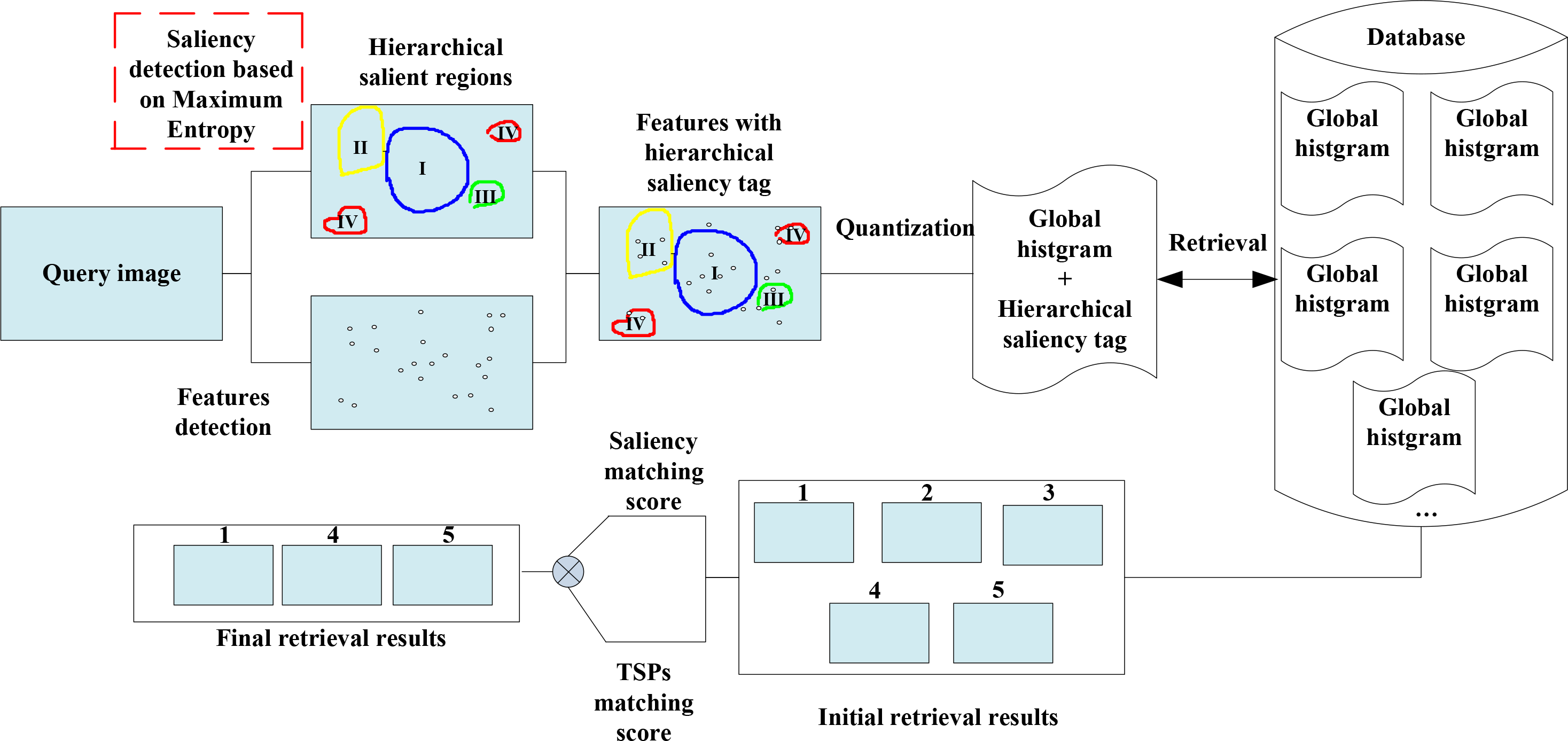
2. The Image Retrieval Framework with Hierarchical Salient Regions Based on Maximum Entropy

Inspired by analyzing visual saliency, this paper extends the image retrieval method based on visual saliency information. We propose to use hierarchical salient regions tags based on the maximum entropy principle. In our image retrieval architecture, retrieval objects of candidate images are not only from one single salient region but from multi-level regions, which could greatly increase the relevance of final retrieval results. The framework of our method is illustrated in Figure 2. Given a query image, first we extract SIFT features [19] and obtain the hierarchical salient regions based on two-dimensional maximum entropy [22], then saliency tags of visual features are obtained by salient region that the visual features are located in. Initial retrieval results are obtained based on the BOW retrieval model [11]. In the geometry verification stage, the initial retrieval list is re-indexed by a new designed spatial pattern scheme weighted by saliency matching results.

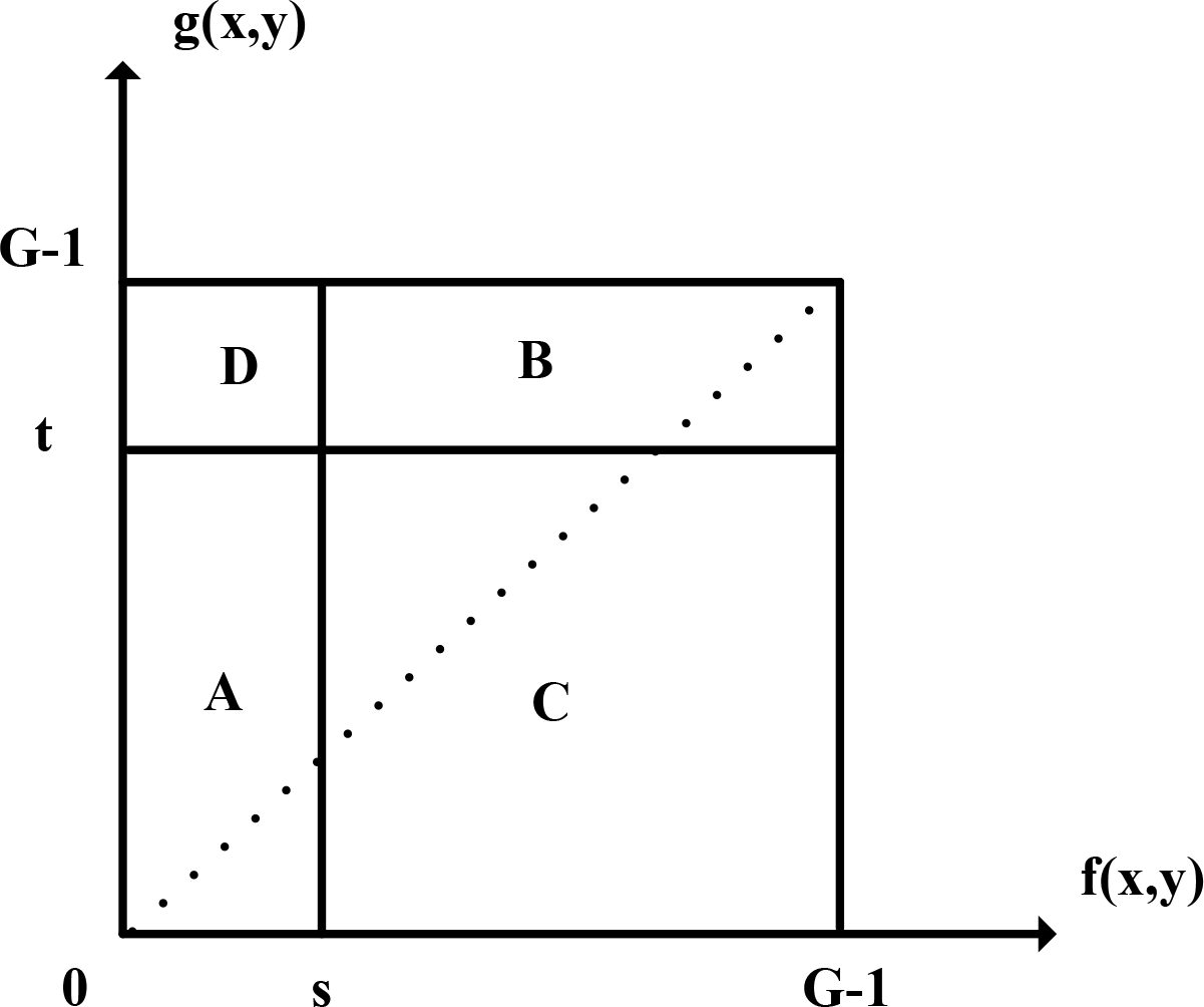
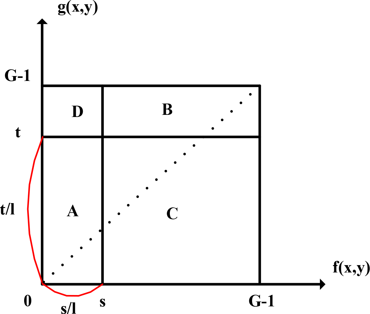
3. Hierarchical Saliency Generation Based on Maximum Entropy Principle

Image segmentation based on thresholds, such as global threshold [23], adaptive threshold [24], the best threshold [25] and entropy method [26] are widely used. In this paper, the two-dimensional maximum entropy principal [22] is applied to segment a saliency map image.

Various kinds of saliency models have been proposed [27–31]. Meanwhile many review articles also refer to these saliency algorithms. In this paper we choose to use the GBVS algorithm [21] for saliency map calculations after considering both accuracy and algorithmic complexity.

First of all, the saliency map is generated by GBVS algorithm, and we consider the saliency map as a grey image and detect multi-level salient regions in it according to the region’s saliency level. A two- dimensional histogram of pixel distribution between the image pixels and the surrounding neighborhood is built. Then the optimal threshold to divide the image into object region and background region is obtained by the maximum entropy criterion. In order to extract multi-level salient regions, we further segment background region by adjusting segmentation threshold. Figure 3 shows the computation process example of a four-level hierarchical salient region.

Given a M × N image f(x, y)(x ≤ M, y ≤ N), a smooth image g(x, y) is generated by using each pixel values in the image and the average pixel values of 8-neighborhood. All grey values are quantized into G levels: 0,1,...,G − 1. We define the joint pixel distribution probability of each pixel in the original image and in the smoothed image.

$$p(i,j)=\frac{r(i,j)}{T},i,j=0,1,\dots ,G-1$$

(1)

where T = M × N and r(i, j) represents the number of pixels with grey value i and average neighborhood pixel grey value j. That results in a two-dimensional histogram as shown in Figure 3.

As shown in Figure 4, any two-dimensional vector (s, t) is used as segmentation threshold. Region A and B represent background and object region, respectively. Region C and D represent edge region and noise region respectively. We approximate region C and D to 0, because edge and noise pixels are in the minority and are far away from the diagonal. Therefore we could use a single threshold vector to divide an input image into object region and background region.

Here we introduce two-dimensional entropy principle to compute the best threshold. A discrete two-dimensional entropy is defined as:

$$H=-{\sum }_i{\sum }_j{p}_{i,j}\mathit{log}{p}_{i,j}$$

(2)

where p_i,j is joint probability density, defined in Equation (1).

Usually the background region and the objective region have different probability distribution as:

$$P_A=\sum _{i=0}^{s-1}\sum _{j=0}^{t-1}{p}_{i,j},\hspace{0.17em}\hspace{0.17em}\hspace{0.17em}\hspace{0.17em}{P}_{\text{o}}=\sum _{i=s}^{G-1}\sum _{j=t}^{G-1}{p}_{i,j}$$

(3)

Therefore the entropy of background is:

$$H_A(s,t)=-\sum _{i=0}^{s-1}\sum _{j=0}^{t-1}\frac{p_{i,j}}{P_A}\mathit{log}\left(\raisebox{1ex}{$p_{i,j}$}\!\left/ \!\raisebox{-1ex}{$P_A$}\right.\right)$$

(4)

The entropy of the object is:

$$H_o(s,t)=-\sum _{i=s}^{G-1}\sum _{j=t}^{G-1}\frac{p_{i,j}}{P_o}\mathit{log}\left(\raisebox{1ex}{$p_{i,j}$}\!\left/ \!\raisebox{-1ex}{$P_o$}\right.\right)$$

(5)

The sum of the entropy of the whole image [22] is:

$$\Phi (s,t)=H_A(s,t)+H_o(s,t)=\mathit{log}[P_A(1-P_A)]+\frac{H_A}{P_A}+\frac{H_L-H_A}{1-P_A}$$

(6)

where P_A presents the probability of the background region, H_A represents the entropy of the background region and H_L shows the entropy of the whole image. The best threshold (s^*, t^*) based on maximum entropy principle must satisfy:

$$(s^{*},t^{*})=\mathit{argma}{\mathit{x}}_{(s,t)}\{\Phi \}$$

(7)

After obtaining the segmentation threshold of the salient map, the usual saliency schemes in image retrieval extract object regions as a query image. However when the retrieval object of a candidate image is located outside the salient region, this approach tends to lose the retrieved information and could even affect the retrieval accuracy. Therefore we propose the concept of hierarchical salient regions to rectify this error.

We investigate the adoption of multi-level salient regions and create salient matching principal by the criterion that more significant area the features are located in, the higher salient matching score they can get. Therefore, for the first step, we need to extract multiple saliency levels. After applying two-dimensional maximum entropy to the original saliency map, the input image could be segmented into a single object region and a background region. As normal retrieval methods only concentrate on the retrieved content inside the object region and neglect the background information, this paper focuses on compensating retrieving background content in order to give higher coverage of the retrieval results.

After extracting the salient target by the two-dimensional maximum entropy principal, if we need to extract l salient levels, we should again compute l − 1 salient levels in the background. This would spend too much time on so many l − 1 iterations, consequently we apply another simple approach to solve this problem, as shown in Figure 5.

In the saliency map of the query image, amounts of nearly black pixels usually exist in the background and are distributed in the (0,0) bin around the two-dimensional histogram. They are not very helpful for image retrieval due to the insignificant information they contain, so we discard the region where the pixels are close to black pixels.

We average the interval (0, s) and (0, t) into l scopes to extract these sub-regions, and discard the most insignificant regions where the grey value f(x, y) is in range of 0 to s/l and the average neighborhood pixel grey value g(x, y) is in range of 0 to t/l. Together with the object region B, l hierarchical salient regions are determined.

4. Geometric Verification Based on Hierarchical Salient Regions and Triangle Spatial Pattern

In this section, we introduce the hierarchical salient regions and spatial features which are used in geometric verification in a large-scale database. First, the initial retrieval list is obtained based on the BOW model. Each visual word has an entry in the index that contains the list of images in which the visual word appears. Additional, we also record the geometric information: the image ID, X-coordinate, Y-coordinate and hierarchical saliency tag. The structure of the inverted file is shown in Figure 6.

We combine the salient tags and visual features to enrich the descriptor content. After the retrieval step, query image has an initial retrieval result list.

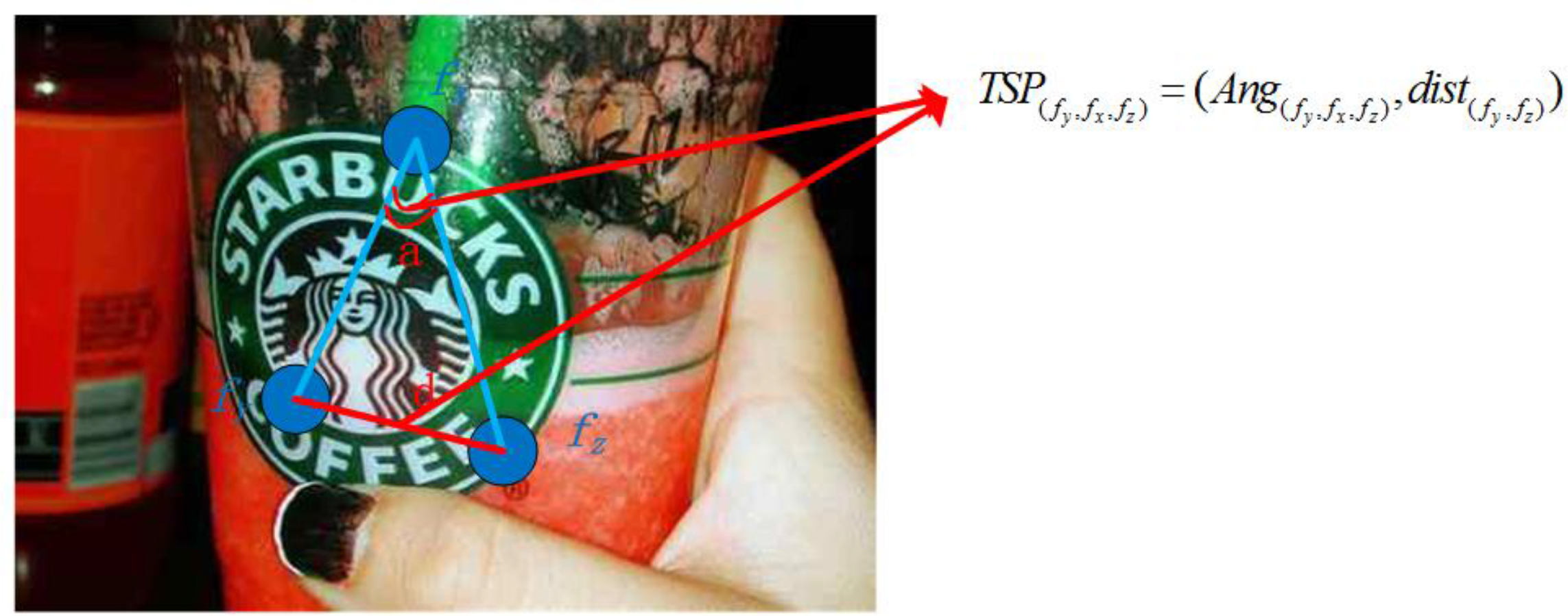
4.1. Triangle Spatial Pattern (TSP)

After SIFT quantization, matched features between two images can be obtained. However the retrieval results are usually polluted by parts of false matches due to quantization errors and visual word ambiguity. Hence, geometry verification is used as a geometric verification step to verify initial retrieval results list. In this paper, we propose to take spatial distribution of matched features into account.

The key idea of our triangle spatial pattern (TSP) is the spatial relationship of SIFT features for spatial consistency verification. We design a spatial pattern as a triangle made up of every three SIFT feature points and examine the similarity of two TSPs by their similarity ratio.

For instance, given an image with N features, (i = 1,2,...,N), The triangle spatial pattern of the three feature points (f_y, f_x, f_z), is defined as: TSP_(fy,fx,fz) = (Ang_(fy,fx,fz),dist_(fy,fz)), 1 ≤ x, y, z ≤ N, as shown in Figure 7.

The angle information is quantized as:

$$\mathit{An}{\mathit{g}}_{(f_y,f_x,f_z)}=\frac{\mathit{dist}{(f_x,f_y)}^2+\mathit{dist}{(f_x,f_z)}^2-\mathit{dist}{(f_y,f_y)}^2}{2\times \mathit{dist}(f_x,f_y)\times \mathit{dist}(f_x,f_z)}$$

(8)

where dist(,)corresponds to the Euclidean distance of two feature points.

If there are m matched visual features within a certain salient level, the number of TSPs in this level is $N=C_m^3$. If the number of matched visual features in a certain level is less than three, TSP matching is not applicable to it. Therefore, match scores of TSP in this saliency level is zero.

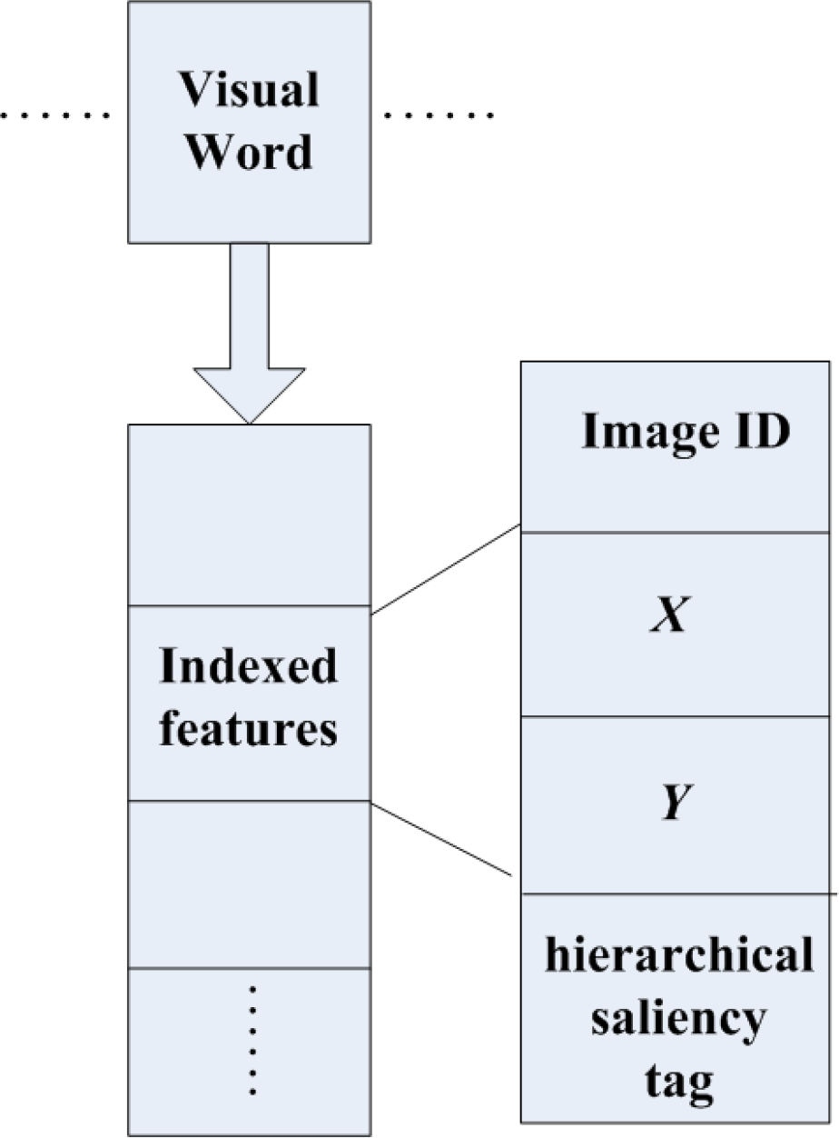
4.2. Geometric Verification with Hierarchical Salient Regions and TSP

In geometric verification, we first calculate TSP matching scores in every single salient level. Then the geometric scores between query image and candidate images are obtained by summing all TSP matching scores weighted by saliency level scores.

Since there is an underlying assumption that the candidate image and query image share some similar parts, or in other words, share some features with consistent geometry, we could compare the number of similar TSPs between images to generate a more accurate retrieval list.

In the geometry verification step, we consider both saliency attributes and spatial relationships represented as TSP. We denote a query image as I_q and a candidate image as I_d. Q = (q_f1, q_f2, ⋯ q_fK) and Q = (d_f1′, d_f2′, ⋯ d_fK′) represent the feature sets in the query image and the candidate image respectively. We get the matched feature-pair as M(q, d) = {(q_fi, d_fi′)| q_fi ∈ Q, d_fi′ ∈ D}, where f_i and f_i′ denote the features in the query image and candidate image.

4.3. Matching TSPs

We firstly measure the similarity degree of angles in TSP_q and TSP_d:

$$S_{\left(\mathit{An}{\mathit{g}}_q,\mathit{An}{\mathit{g}}_d\right)}=\left\{\begin{array}{c}\frac{\mathit{Ang}(q_{f_y},q_{f_x},q_{f_z})}{\mathit{Ang}(d_{f_y},d_{f_x},d_{f_z})},\mathit{Ang}(d_{{f_y}^{\prime }},d_{{f_x}^{\prime }},d_{{f_z}^{\prime }})\ne 0\\ 0,\mathit{Ang}(q_{f_y},q_{f_x},q_{f_z})\ne 0,\mathit{Ang}(d_{{f_y}^{\prime }},d_{{f_x}^{\prime }},d_{{f_z}^{\prime }})=0\\ 1,\mathit{Ang}(q_{f_y},q_{f_x},q_{f_z})=\mathit{Ang}(d_{{f_y}^{\prime }},d_{{f_x}^{\prime }},d_{{f_z}^{\prime }})=0\end{array}|\begin{array}{c}\left(q_{f_x},d_{{f_x}^{\prime }}\right)\in M(q,d)\\ \left(q_{f_y},d_{{f_y}^{\prime }}\right)\in M(q,d)\\ \left(q_{f_z},d_{{f_z}^{\prime }}\right)\in M(q,d)\end{array}\right\}$$

(9)

S_(Angq,Angd) is computed as the angle cosine ratio between TSP_q and TSP_d. However, there are two exceptions: when the numerator and the denominator are both zero, S_(Angq,Angd) is equal to 1. Otherwise, the value of S_(Angq,Angd) is zero. Furthermore, we compute the distance ratio of the opposite side. Obviously, the distance ratio is proportional to the scale transformation factor. We compute edge similarity as:

$$S_{(\mathit{edg}{\mathit{e}}_q,\mathit{edg}{\mathit{e}}_d)}=\left\{\mathit{log}\left(\frac{\mathit{dist}\left(q_{f_y},q_{f_z}\right)}{\mathit{dist}\left(d_{{f_y}^{\prime }},d_{{f_z}^{\prime }}\right)}\right)\left||S_{\left(\mathit{An}{\mathit{g}}_q,\mathit{An}{\mathit{g}}_d\right)}-1\right|<\varepsilon \right\}$$

(10)

where |S_(Angq,Angd) − 1| < ε represents the angle component of TSP_p and TSP_d should satisfy the similarity relationship. We build a histogram of the distance ratio S_{(edgeq,edged)}:

$$C(\alpha )=\sum _{Z\in S_{\left(\mathit{edg}{\mathit{e}}_q,\mathit{edg}{\mathit{e}}_d\right)}}\mathit{Hist}\left(a\le Z\le a+b\right)$$

(11)

Hist(,)is the indicator function, and a corresponds to the scale ratio difference. We implement Equation (11) as the histogram with the interval b. C(α) represents the height of the a-th bin.

$$\mathit{Scor}{\mathit{e}}_{\mathit{TSP}}=\mathit{ma}{\mathit{x}}_{a}C(a)$$

(12)

The maximum value of C in all histogram bins is used as the TSPs matching score. This score is also used as the matching scores of a certain saliency level in geometric verification.

4.4. Re-Rank Score of a Candidate Image

Finally, the re-rank score of candidate image I_d is calculated by weighting TSPs matching score with saliency matching score W_{saliencylevel}. Assume there are l-level salient regions in the query image, so the final re-rank score of a candidate image is computed as:

$$\mathit{FinaScor}{\mathit{e}}_{I_d}={\sum }_{\mathit{level}=1}^l{W}_{\mathit{saliencylevel}}(\mathit{level})*\mathit{Scor}{\mathit{e}}_{(\mathit{level},\mathit{TSP})}$$

(13)

where W_{saliencylevel} means the saliency weight and Score_(level,TSP) represents matching score of TSPs in the level-th saliency level:

$$W_{\mathit{saliencylevel}}(\mathit{level})=\frac{l}{\mathit{level}}*\frac{1}{{\sum }_{s=1}^{l}s}$$

(14)

where l shows the number of hierarchical salient level in section 3, level represents the level-th salient region.

5. Experimental Section

The evaluation of our hierarchical geometric verification based on maximum entropy saliency is based on the two important factors in image retrieval: retrieval accuracy and search time in the geometric verification stage.

5.1. Datasets

We first evaluate the relationship between the saliency level value l and retrieval performance by adjusting the level value. By doing so, we could get the level value with the best retrieval performance. In experiments, we use traditional a BOW retrieval model [11] and TSP without saliency in Section 4.2 as contrasts. The experiments are evaluated on a publicly available image retrieval datasets: DupImage [32]. We add some relevant images from Flickr [33], and crawled ten thousand images from the dataset [34] as distracters. In our experiments, the top 1000 initial retrieval images are verified in the geometry verification stage.

5.2. Experiment Preparations

Our method is based on the traditional BOW retrieval model, and we adopt SIFT features as visual features for local image representation. Key points are detected with the Difference-of-Gaussian detector, and 128-dimensional SIFT descriptors are extracted accordingly. Meanwhile location information of the key points is recorded as a part of visual features. Before feature extraction, large images are scaled to no larger than 500 × 500. We apply the hierarchical visual vocabulary tree approach for visual word generation [35] as our baseline. We use a vocabulary of 100 K visual words. We experimented with different sizes (both larger and smaller) of visual word vocabularies in our dataset, and found it is the best choice. We use an inverted file structure to index the images. As illustrated in Figure 6, each visual word is linked with a list of indexed features that are quantized. Each indexed feature records the ID of the image, feature location, and hierarchical saliency tag.

5.3. Evaluation Protocol

We evaluate the performance of our method by the mAP criteria [36] and perform the experiments on a server with 3.20 GHz CPU and 8 GB memory running MatlabR2012a. In the following evaluation, we select 100 representative images from each group of datasets as our queries, and compute each average mAP and take the mean value over all queries.

The mAP criteria is computed as:

$$\mathit{mAP}=\frac{{\sum }_{i=1}^n\frac{i}{\mathit{rank}(i)}}{n}$$

(15)

where n represents the number of positive retrieval images in database with given query image, rank(i) is the rank value of the i-th positive retrieval image in the final retrieval results.

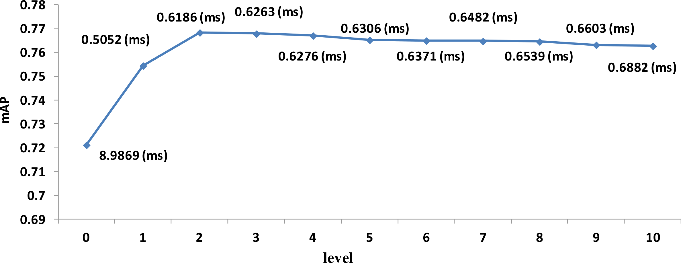
5.4. Evaluation for Level in Hierarchical Saliency

The performance of our approach related to the different level values is shown in Figure 8. Meanwhile the average time cost per query of all approaches in geometry verification is also represented.

In the geometric verification step, the factor level works to cast geometric consistency constraints on the relative spatial positions between matched features. We also need to evaluate its value impact on retrieval performance so as to select the optimal value. Intuitively, the mAP achieves the best result when the level is 2. By analyzing the influence of saliency level to retrieval performance, we can conclude that the higher we set the saliency level, the more segmented regions and the more remained features are computed. Since our geometric verification method mainly relies on the detection of SIFT features, the impact of SIFT matching errors in geometric verification between query and retrieved images is illustrated in Figure 9. It is observed that, with the increasing of salient regions, the mAP performance first rises, and then gradually drops after the level reaches 2. The reason is the saliency method could discard the useless features which are located in the most insignificant regions. It avoids the distraction of false matched features for the geometric verification method and improves the retrieval accuracy by these useful features. However when part of the retrieval target in images is out of the salient regions, the less salient regions there are, the more retrieving content would be ignored, and this would affect the retrieval accuracy. Hence, the hierarchical saliency is considered to retain the whole information of the retrieval object. As shown in Figure 8, the mAP achieves the best result when level is 2, which represents that two saliency levels could persist in the fairly complete information of retrieval objects and also could filter the more redundant matches, but as the level increases, the mAP performance gradually drops after the level reaches 2. The reason might be that the more hierarchical saliency regions we use, the more redundant matches would be computed that will eventually affect the retrieval accuracy. Meanwhile, when computing the matching scores of TSPs in hierarchical salient regions, the larger the saliency level is set, the more time will be consumed through all levels of the hierarchical saliency regions.

5.5. Hierarchical Saliency’s Effect in Image Retrieval

We select the appropriate salient level in Section 5.4 by considering both retrieval precision and time consumption. In performance comparison experiments, we select level = 2, when the mAP is better than other saliency levels. HGV is compared to the traditional BOW retrieval model [11] introduced in Section 5.3 and the TSP without any hierarchical saliency in Section 4.2. Figure 10 shows the mAP comparison in six groups of the DupImage database for the three methods. Comparison in time consumption is denoted in

Table 1. Comparison of time consuming for four methods in common case.

Method	Features exaction (query image) [s]	Retrieval [s]	Per retrieval image Geometric verification [ms]	Total time [s]
BOW	0.1903	0.0053	-	0.2043
TSP	0.1903	0.0053	8.9869	9.1825
HGV (level = 2)	1.0406	0.0053	0.6186	1.6645

. The examples of the six groups are illustrated in Figure 11.

From the comparison results, it can be concluded that our method not only improves retrieval precision, but also reduces the time consumed in the geometric verification step. TSP improves the retrieval precision due to the introduction of spatial layout of visual features. It fills the spatial information which the traditional BOW model lacks due to the quantization visual words. After that, the hierarchical saliency mechanism is taken into consideration. When the retrieval object in a salient region is incomplete or some retrieval objects are located in background regions, the hierarchical saliency method can keep the retrieval object information. From Table 1, we can see, the time consumed in geometric verification step has been reduced (from TSP’s 8.9869 ms to 0.6186), because we discard the features which are located in the most insignificant region, so that the less features are computed in the geometric verification step, which speeds up retrieval process while improving the retrieval accuracy.

Figure 12 shows the final retrieval result of HGV and other methods. The retrieval results containing large changes in color, scale and rotation demonstrate the effectiveness of our method in complex image transformation.

5.6. Hierarchical Saliency’s Effect on Other Geometry Verification Methods

Finally, we perform some other geometry verification methods like LGSS [20], WGC [13] and LGC [17] to verify the effectiveness of HGV. The parameters of the comparison methods are based on the relevant papers.

From the previous comparison results, it can be concluded that hierarchical saliency method is a common approach to improve the precision in image retrieval as denoted in Figure 14. The lower part shows the mAP performance of all retrieval methods without adding any saliency; with the addition of hierarchical saliency, the mAP performance is improved, as illustrated in the upper part.

In Figure 13, the traditional BOW retrieval method quantified visual words may reduce the discriminative power of the local features and do not capture the spatial relationship among local features, thus leading to many false matched pairs and affecting the retrieval performance. Therefore, our method applies a multi-point spatial layout to compute the geometric consistency. It can reduce the probability of misjudgment of matched features compared to the LGSS method [20] due to the instability of computing matched features with two point encoding. WGC has strong assumptions and can only work under uniform transformations between the query image and candidate images. LGC couldn’t make the best of the local similar characteristic of deformations due to the high size of visual words (10⁵) and this results in calculating the transformation matrix less accurately. It is also affects the retrieval accuracy.

Table 2. Comparison of time consumption for other geometric verification methods.

Method	Per retrieval image Geometric verification [ms]
LGSS	0.3660
LGSS + hierachical saliency (level = 2)	0.3127
WGC	0.2285
WGC + hierachical saliency (level = 2)	0.2789
LGC	0.6597
LGC + hierachical saliency (level = 2)	0.6358

shows the average query time per image for these methods. We can see that the performance of WGC, LGSS and LGC. Compared to WGC (0.2258 ms), LGSS (0.3660 ms) has to calculate the distance ratio instead of simple addition and subtraction of two points, and LGC (0.6597 ms) has to additionally calculate the local geometric similarity. Due to the introduction of hierarchical saliency, many redundant matched features are discarded, which reduces the geometric verification computations of LGSS (0.3127 ms) and LGC (0.6358 ms), but the geometric verification computation of WGC (0.2285 ms) with hierarchical saliency is increased, because the time consumed in searching matched features with the same hierarchical saliency tag is more than through using less feature points in WGC.

6. Conclusions

We investigate the Hierarchical Geometry Verification based on Maximum Entropy Saliency in image retrieval. Most state-of-the-art image retrieval methods based on the BOW model ignore the spatial relationships among local features, thus decreasing retrieval precision. In this paper, we define a triangle spatial pattern to describe the spatial layout of visual features to verify the features’ geometric relationships in the geometric verification step. However, this consumes more time due to the high computing complexity. Therefore, we introduce the Hierarchical Saliency based on Maximum Entropy mechanism to reduce the number of features involved in each segmented region for geometry verification. To filter the redundant matched features and retain the useful visual features, only matched features in some more saliency levels are kept to be evaluated, which can increase the retrieval speed and improve the retrieval accuracy. In our experiment, our method outperforms state-of-art methods in retrieval accuracy such as LGSS, WGC and LGC, and take less time in geometric verification. However, when the complete part of retrieval object is located in a less prominent area, too many hierarchical saliency regions would destroy the integrity of the retrieval object while ignoring the positive match. In our future work, we will study a new object contour preserving method to distill the hierarchical saliency region. Hopefully, it will be helpful to increase retrieval performance.

References

1. Datta, R.; Joshi, D.; Li, J.; Wang, J.Z. Image retrieval: Ideas, influences, and trends of the new age. ACM Comput. Surv 2008, 40. [Google Scholar] [CrossRef]
2. Bhandari, K.; Dugar, N.; Jain, N.; Shetty, N. A novel high performance multi-modal approach for content based image retrieval. In Proceedings of the International Conference and Workshop on Emerging Trends in Technology 2010, ICWET 2010, Mumbai, Maharashtra, India, 26–27 February 2010; Association for Computing Machinery: Mumbai, Maharashtra, India, 2010; pp. 253–256. [Google Scholar]
3. Fiala, M. Using normalized interest point trajectories over scale for image search. In Proceedings of the 3rd Canadian Conference on Computer and Robot Vision, CRV 2006, Quebec City, QC, Canada, 7–9 June 2006.
4. Zhang, Z.-H.; Quan, Y.; Li, W.-H.; Guo, W. A new content-based image retrieval. In Proceedings of the 2006 International Conference on Machine Learning and Cybernetics, Dalian, China, 13–16 August 2006; pp. 4013–4018.
5. Yue, L.; Wan, S.; Jin, P. An approach for image retrieval based on visual saliency. In Proceedings of International Conference on Image Analysis and Signal Processing, Taizhou, China, 11–12 April 2009; pp. 172–175.
6. Liu, Y.; Zhang, D.; Lu, G.; Ma, W.-Y. A survey of content-based image retrieval with high-level semantics. Pattern Recogn 2007, 40, 262–282. [Google Scholar]
7. Rutishauser, U.; Walther, D.; Koch, C.; Perona, P. Is bottom-up attention useful for object recognition? In Proceedings of the 2004 IEEE Computer Society Conference on Computer Vision and Pattern Recognition, CVPR 2004, Washington, DC, USA, 27 June–2 July 2004; 32, pp. II-37–II-44.
8. Walther, D.; Koch, C. Modeling attention to salient proto-objects. Neural Netw 2006, 19, 1395–1407. [Google Scholar]
9. Kadir, T.; Brady, M. Saliency, scale and image description. Int. J. Comput. Vis 2001, 45, 83–105. [Google Scholar]
10. Soares, R.D.C.; Silva, I.R.D.; Guliato, D. Spatial locality weighting of features using saliency map with a bag-of-visual-words approach. In Proceedings of the 2012 IEEE 24th International Conference on Tools with Artificial Intelligence, ICTAI 2012, Athens, Greece, 7–9 November 2012; pp. 1070–1075.
11. Sivic, J.; Zisserman, A. Video Google: A text retrieval approach to object matching in videos. Proceedings of the 2003 Ninth IEEE International Conference on Computer Vision, Nice, France, 11–17 October 2003; pp. 1470–1477.
12. Chum, O.; Perdoch, M.; Matas, J. Geometric min-hashing: Finding a (thick) needle in a haystack. In Proceedings of the 2009 IEEE Conference on Computer Vision and Pattern Recognition, CVPR 2009, Miami, FL, USA, 20–25 June 2009; pp. 17–24.
13. Jegou, H.; Douze, M.; Schmid, C. Hamming embedding and weak geometric consistency for large scale image search. In Computer Vision–ECCV 2008; Springer: New York, NY, USA, 2008; pp. 304–317. [Google Scholar]
14. Philbin, J.; Chum, O.; Isard, M.; Sivic, J.; Zisserman, A. Object retrieval with large vocabularies and fast spatial matching. In Proceedings of the 2007 IEEE Conference on Computer Vision and Pattern Recognition, CVPR 2007, Minneapolis, MN, USA, 18–23 June 2007; pp. 1–8.
15. Wu, Z.; Ke, Q.; Isard, M.; Sun, J. Bundling features for large scale partial-duplicate web image search. In Proceedings of the 2009 IEEE Conference on Computer Vision and Pattern Recognition, CVPR 2009, Miami, FL, USA, 20–25 June 2009; pp. 25–32.
16. Zhao, W.-L.; Wu, X.; Ngo, C.-W. On the annotation of web videos by efficient near-duplicate search. IEEE Trans. Multimed 2010, 12, 448–461. [Google Scholar]
17. Xie, H.; Gao, K.; Zhang, Y.; Li, J. Local geometric consistency constraint for image retrieval. In Proceedings of the 2011 18th IEEE International Conference on Image Processing, ICIP 2011, Brussels, Belgium, 11–14 September 2011; pp. 101–104.
18. Fischler, M.A.; Bolles, R.C. Random sample consensus: A paradigm for model fitting with applications to image analysis and automated cartography. Commun. ACM 1981, 24, 381–395. [Google Scholar]
19. Lowe, D.G. Distinctive image features from scale-invariant keypoints. Int. J. Comput. Vis 2004, 60, 91–110. [Google Scholar]
20. Tsai, S.S.; Chen, D.; Takacs, G.; Chandrasekhar, V.; Vedantham, R.; Grzeszczuk, R.; Girod, B. Fast geometric re-ranking for image-based retrieval. In Proceedings of the 2010 17th IEEE International Conference on Image Processing, ICIP 2010, Hong Kong, China, 26–29 September 2010; pp. 1029–1032.
21. Harel, J.; Koch, C.; Perona, P. Graph-based visual saliency. In Proceedings of the Advances in neural information processing systems, Vancouver, BC, Canada, 4–7 December 2006; pp. 545–552.
22. Luo, G.; Huang, W.; Li, S. 2-D maximum entropy spermatozoa image segmentation based on Canny operator. In Proceedings of the 2010 IEEE International Conference on Intelligent Computing and Integrated Systems, ICISS 2010, Guilin, China, 22–24 October 2010; pp. 243–246.
23. Wuhib, F.; Dam, M.; Stadler, R. Decentralized detection of global threshold crossings using aggregation trees. Comput. Netw 2008, 52, 1745–1761. [Google Scholar]
24. Zhang, B.; Zhong, B.; Cao, Y. Complex background modeling based on texture pattern flow with adaptive threshold propagation. J. Vis. Commun. Image Represent 2011, 22, 516–521. [Google Scholar]
25. Chao, D.C.; Scheinhorn, D.J. Determining the best threshold of rapid shallow breathing index in a therapist-implemented patient-specific weaning protocol. Respir. Care 2007, 52, 159–165. [Google Scholar]
26. Kapur, J.; Sahoo, P.K.; Wong, A. A new method for gray-level picture thresholding using the entropy of the histogram. Comput. Vis. Graph. Image Process 1985, 29, 273–285. [Google Scholar]
27. Itti, L.; Koch, C.; Niebur, E. A model of saliency-based visual attention for rapid scene analysis. IEEE Trans. Pattern Anal. Mach. Intell 1998, 20, 1254–1259. [Google Scholar]
28. Milanese, R.; Wechsler, H.; Gill, S.; Bost, J.-M.; Pun, T. Integration of bottom-up and top-down cues for visual attention using non-linear relaxation. In Proceedings of the 1994 IEEE Computer Society Conference on Computer Vision and Pattern Recognition, CVPR 1994, Seattle, WA, USA, 21–23 June 1994; pp. 781–785.
29. Maki, A.; Nordlund, P.; Eklundh, J.-O. A computational model of depth-based attention. In Proceedings of the 1996 13th International Conference on Pattern Recognition, Vienna, Austria, 25–29 August 1996; pp. 734–739.
30. Gopalakrishnan, V.; Hu, Y.; Rajan, D. Random walks on graphs to model saliency in images. In Proceedings of the 2009 IEEE Conference on Computer Vision and Pattern Recognition, CVPR 2009, Miami, FL, USA, 20–25 June 2009; pp. 1698–1705.
31. Costa, L.D.F. Visual saliency and attention as random walks on complex networks. 2006. arXiv preprint physics/0603025. [Google Scholar]
32. DupImage. Available online: https://dl.dropboxusercontent.com/u/42311725/DupGroundTruthDataset.rar. (accessed on 10 July 2014).
33. Flickr. Available online: http://www.flickr.com/ (accessed on 10 July 2014).
34. Image.vary.jpg. Available online: http://www.db.stanford.edu/~wangz/image.vary.jpg.tar (accessed on 10 July 2014).
35. Nister, D.; Stewenius, H. Scalable recognition with a vocabulary tree. In Proceedings of the 2006 IEEE Computer Society Conference on Computer Vision and Pattern Recognition, CVPR 2006, New York, NY, USA, 17–22 June 2006; pp. 2161–2168.
36. Philbin, J.; Chum, O.; Isard, M.; Sivic, J.; Zisserman, A. Object retrieval with large vocabularies and fast spatial matching. In Proceedings of the 2007 IEEE Computer Society Conference on Computer Vision and Pattern Recognition, CVPR 2007, Minneapolis, MN, USA, 17–22 June 2007.
Figure 1. Saliency example of the query image. (a) Original image. (b) Salient region. (ce) Hierarchical salient regions. The first line on the right hand of the arrow shows the saliency model only detects single salient region; The second line on the right arrow denotes the hierarchical saliency model.
Entropy 16 03848f1
Figure 2. Retrieval framework.
Entropy 16 03848f2
Figure 3. The process of computing four-level hierarchical salient regions based on maximum entropy principal. (a) Original Image; (b) Saliency map generated by GBVS; (c) Two-dimensional pixel distribution histogram of saliency map image; (d) Four-level hierarchical salient regions.
Entropy 16 03848f3
Figure 4. The two-dimensional histogram.
Entropy 16 03848f4
Figure 5. An example of a hierarchical salient area.
Entropy 16 03848f5
Figure 6. Inverted file structure for index. The image ID means where the visual word. appears, the location information(X,Y) and hierarchical saliency tag are recorded by each indexed features.
Entropy 16 03848f6
Figure 7. The attribute of spatial features.
Entropy 16 03848f7
Figure 8. Comparison of mAP curve for different methods.
Entropy 16 03848f8
Figure 9. Example of matched pairs between query image and retrieval image. (a) Query image; (b) Retrieval image. In fact, the matched pair between feature 3 in Figure 9(a) and feature 3′ in Figure 9(b) is false. We propose the geometric verification method with three features. With this method, it will not compute the geometric similar scores containing matched pair (3, 3′) by judging whether the angles are similar in the triangle pattern.
Entropy 16 03848f9
Figure 10. Comparison of mAP for three methods.
Entropy 16 03848f10
Figure 11. Retrieval examples of six groups [3233].
Entropy 16 03848f11
Figure 12. Retrieval results of different methods (All images are from datasets [3234]). (a) BOW; (b) LGSS; (c) WGC; (d) LGC; (e) TSP; (f) HGV (level = 2).
Entropy 16 03848f12aEntropy 16 03848f12b
Figure 13. Comparison of mAP with other geometric verification methods.
Entropy 16 03848f13
Figure 14. Comparison of mAP for different methods.
Entropy 16 03848f14