Exact Negative Solutions for Guyer–Krumhansl Type Equation and the Maximum Principle Violation

Department of Theoretical Physics, Faculty of Physics, M.V.Lomonosov Moscow State University, Leninskie Gory, Moscow 119991, Russia
Entropy 2017, 19(9), 440; https://doi.org/10.3390/e19090440
Submission received: 22 July 2017
/
Revised: 17 August 2017
/
Accepted: 21 August 2017
/
Published: 24 August 2017
(This article belongs to the Special Issue Selected Papers from 14th Joint European Thermodynamics Conference)
Abstract
:Heat propagation in the Guyer–Krumhansl model is studied. The exact analytical solutions for the one-dimensional Guyer–Krumhansl equation are obtained. The operational formalism is employed. Some examples of initial functions are considered, modeling various initial heat pulses and distributions. The effect of the ballistic heat transfer in an over–diffusive regime is elucidated. The behavior of the solutions in such a regime is explored. The maximum principle and its violation for the obtained solutions are discussed in the framework of heat conduction. Examples of negative solutions for the Guyer–Krumhansl equation are demonstrated.
1. Introduction
Heat conduction is one of the most common physical processes encountered in everyday life. Under normal conditions in macroscopic samples of relatively homogeneous materials the Fourier law describes well heat transport, linearly relating the temperature change with the heat flux [1]. At low temperatures <15 K in some crystals and in highly inhomogeneous media even at normal conditions the Fourier law does not hold. It was first noted by Onsager [2], that Fourier law could be just an approximation, which ignores the time needed for the heat flux acceleration once the temperature has changed. In this way one of the main flaws of the Fourier law was described, i.e., an immediate rise of the heat flux in the whole body at the same time. Beyond Fourier law the most significant physical phenomena is, perhaps, the Second Sound [3], first found in heat pulse propagation experiments in crystals [4,5,6,7]. The description of this phenomenon was given by Cattaneo [8,9], who proposed the proper equation for phonon heat waves, where DT is the heat conductivity and τ is the relaxation time. The velocity of the heat waves propagation in matter in Cattaneo’s model is finite: and therefore the heat flux changes at finite rate, following the temperature change at the boundary. The respective delay τ, in heat flux change after the temperature gradient was applied, is the property of the matter and is associated with phonon–phonon interactions. The Cattaneo model was not flawless (see, for example, [10,11,12,13,14]) and its predictions did not exactly agree with experiments, giving wrong values for the second sound speed in Bi and Na F crystals at low temperatures. The model of Cattaneo was succeeded by the model, developed by Guyer and Krumhansl (GK) [15], which in one dimension reduces to the following equation for the temperature [16]:
where for GK equation; the linear term presumes the heat sources in Equation (1). We do not dwell on the underlying physical mechanisms for the GK model, but just note that additionally to the phonon–phonon interactions in the Cattaneo model, the GK model includes one more mechanism for the heat transfer, acting at the scales L, comparable with the phonon free path l [17,18], and describing the phenomena at the boundary of the media, which was treated neither by Fourier [1] nor by Kasimir [19]. The abovementioned ballistic conditions in the framework of the phonon theory mean that the system scale is of the order of the mean free path of phonons and they are observed in low-dimensional systems, such as ultrathin film, in nanowires, in graphene ribbons and in carbon nanotubes, in silicon threads, etc. [20,21,22,23,24]. Recently it has been shown that the GK equation also applies for the description of heat conduction in highly inhomogeneous and porous matter at other than very low temperatures [25,26,27,28,29,30,31,32], despite the fact there is neither an evident phonon mechanism, nor ballistic conditions present. Modeling of the GK phenomena and heat transfer so far has been conducted mostly by numerical methods [33,34,35,36] and considered in a more general context [37]. In what follows we propose pure analytical exact solutions for GK equations, which, while being particular, explain some of the bizarre features of non-Fourier heat conduction and even go under zero temperature point in some cases.
2. Heat Conduction Operator
With the use of advanced mathematical methods, such as the operational approach to differential exponential operators, combined with Laplace and other integral transforms as well as special functions for differential equations (DE) solution [38,39,40,41] one can obtain particular analytical solutions for a broad range of DE, exactly accounting for all the parameters, describing relevant physical systems.
Theoretical aspects of the heat operator :
were explored by Srivastava [42]. This operator provides the solution of the Fourier Equation:
by means of Gauss transforms with the initial condition (see [38,41]):
For the initial Gaussian distribution we readily obtain the result of the action of the heat operator on it as follows:
and for the Dirac δ-function we have
The heat operator has applications beyond the heat transport; the analogy can be traced to the quantum-mechanical equation process of an electric charge diffusion under a potential barrier, which in the presence of electrostatic field is described as follows:
This in fact means the imaginary time scale in Schrödinger equation [43]. The solution of Equation (7) is obtained by the action of the heat operator on the initial function and consequent action of the operator :
where , . In quantum mechanics the above solution has the meaning of the probability amplitude for the charge to appear in the point x at the moment t, moving from the point x = 0 at the moment t = 0. Same regards the concentration of the particles, diffusing in the electric field under the potential barrier, provided their interaction with each other can be neglected. For an arbitrary function f the solution is given by the convolution of this function with the kernel χ as follows:
where the kernel χ represents the solution of Equation (9) for the initial δ-function :
3. Exact Operational Solution for Guyer–Krumhansl Equation
The one-dimensional Guyer–Krumhansl equation for the temperature, Equation (1), can be conveniently written in the following form:
where , , is the Fourier heat conductivity, is the ballistic type heat conductivity; the term ballistic will be used for for definiteness even when phonon transport does not apply. GK equation is in fact the particular case of the following more general type of equation:
where is the differential operator, acting on x coordinate. Applying Laplace transforms, we obtain the following exact solution in the form of the integral, containing several operational exponents, consequently transforming the initial function :
provided the integral converges. For and for the operator we have the well-known one-dimensional telegraphers equation (TE):
which solution was proposed, for example, in [49]. The particular, bounded and vanishing at infinite time solution for Equation (14) can be obtained from Equation (13) by substituting proper operator in it. The more general solution for Equation (14) reads:
where and are determined from the initial conditions. For GK equation, Equations (1) and (11), and for a particular operational solution reads as follows [50]:
The second branch of the solution, satisfying the initial condition , can be obtained upon simultaneous substitution . In what follows we will study heat conduction in the framework of GK model and employ the above sketched formalism with the exact solutions.
Above we have mentioned that the initial δ-function plays fundamental role for the heat operator and allows obtaining exact solutions for equations, containing differential operator . In the context of heat conduction the initial distribution models the point-like laser pulse heating. This technique is well established for heat conduction experiments [51], thus exact solutions for heat equations with have particular value.
The exact particular solution for the telegrapher’s Equation (14) with initial Dirac δ-function was obtained by the operational method and explored in [52]. For GK Equations (1) and (11) the solution for was obtained in the form of the integral in [50]:
where:
and C1,2 = const, determined from the initial condition and both signs ± are possible in the integral.
For the initial monomial the action of the heat operator yields Hermite polynomials of two variables. Proper solution of the TE was explored in [44,45,52,53]. These studies constituted the base for the subsequent development of the theory of relevant relativistic heat polynomials [54]. For the GK type Equation (1) with the serial initial function , the solution also takes the form of the series
where C1,2 are determined from initial conditions and are the Hermite polynomials of two variables [55,56]
The simplest example of yields:
where the constants C1,2 are determined from initial conditions. The exact solution for the exponential monomial can be obtained with the help of the following identity:
For we obtain the following integral:
where C1,2 = const are determined from initial conditions, , , , , . The result of the integration in Equation (23) with account for Equation (20) reads in terms of elementary functions, but it is cumbersome. For , we obtain:
where .
For the following function: , (note, that and ), which can be viewed as an initial isolated spatial smooth heat pulse, the GK equation has the following solution:
where the constants C1,2 can be determined from proper boundary or initial conditions.
4. Violation of Maximum Principle and Negative Solutions in GK Equation
Considering GK equation, particular attention should be paid to the values of the coefficients in it to recognize the main contributing term and the relevant physical background of the heat transfer in each case. Depending on the values of the constants α, ε, δ one or the other heat transport mechanism contributes more or less. Note, also, that for the GK equation solution also satisfies the Fourier heat equation. Due to the fact that GK equation, which was originally derived in the framework of phonon theory, appears to describe not only systems at low temperature and reduced dimension, where the ballistic conditions can be realized, but it also describes heat condition in macroscopic samples at room temperature, where we cannot talk about phonons, we have to clarify that the regime, in which the condition holds should rather be called over diffusive, following [27]. In what follows we will demonstrate that the behavior of some solutions for GK equation becomes unusual from thermodynamic point of view, and we will develop this topic, earlier touched on in [57]. We do not intend to consider here complicated cases since the relevant calculations are cumbersome, but we will just illustrate the possibility of bizarre solutions, considering the simple case of the solution for :
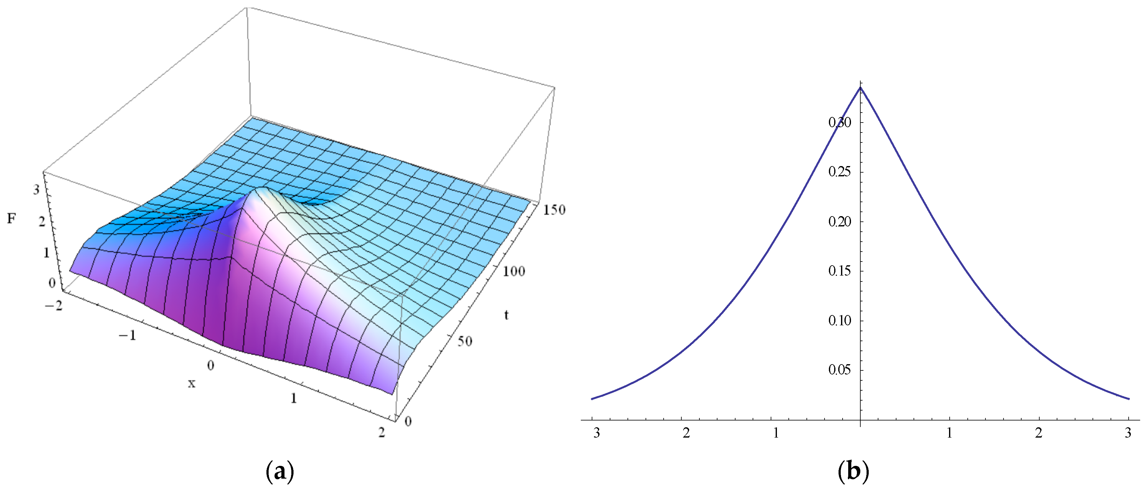
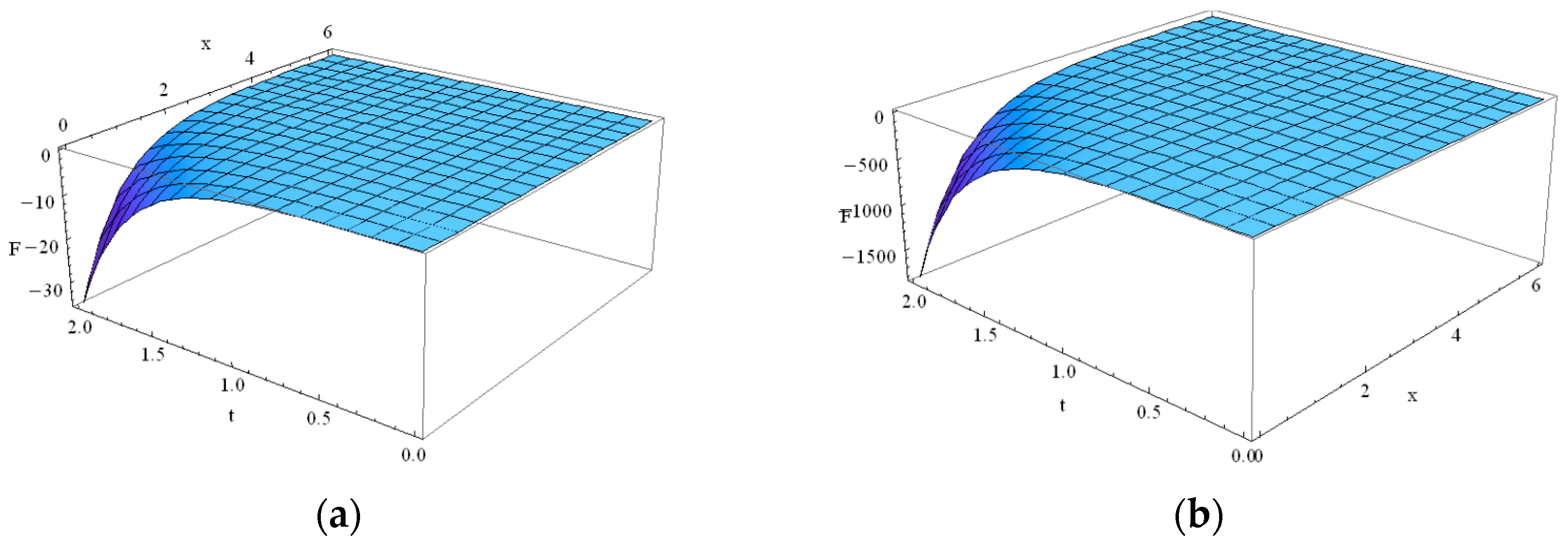
One branch of the solution for α = ε = δ = 1, κ = −0.5 is shown in Figure 1a. In this case the contribution of the Fourier, Cattaneo and ballistic terms in Equation (11) are of comparable with each other order: τ = kT = kb = 1, μ = +0.1. Despite that we observe in Figure 1 the solution, developing from the initial function , which reaches its maximum inside the domain and then fades out, thus violating maximum principle
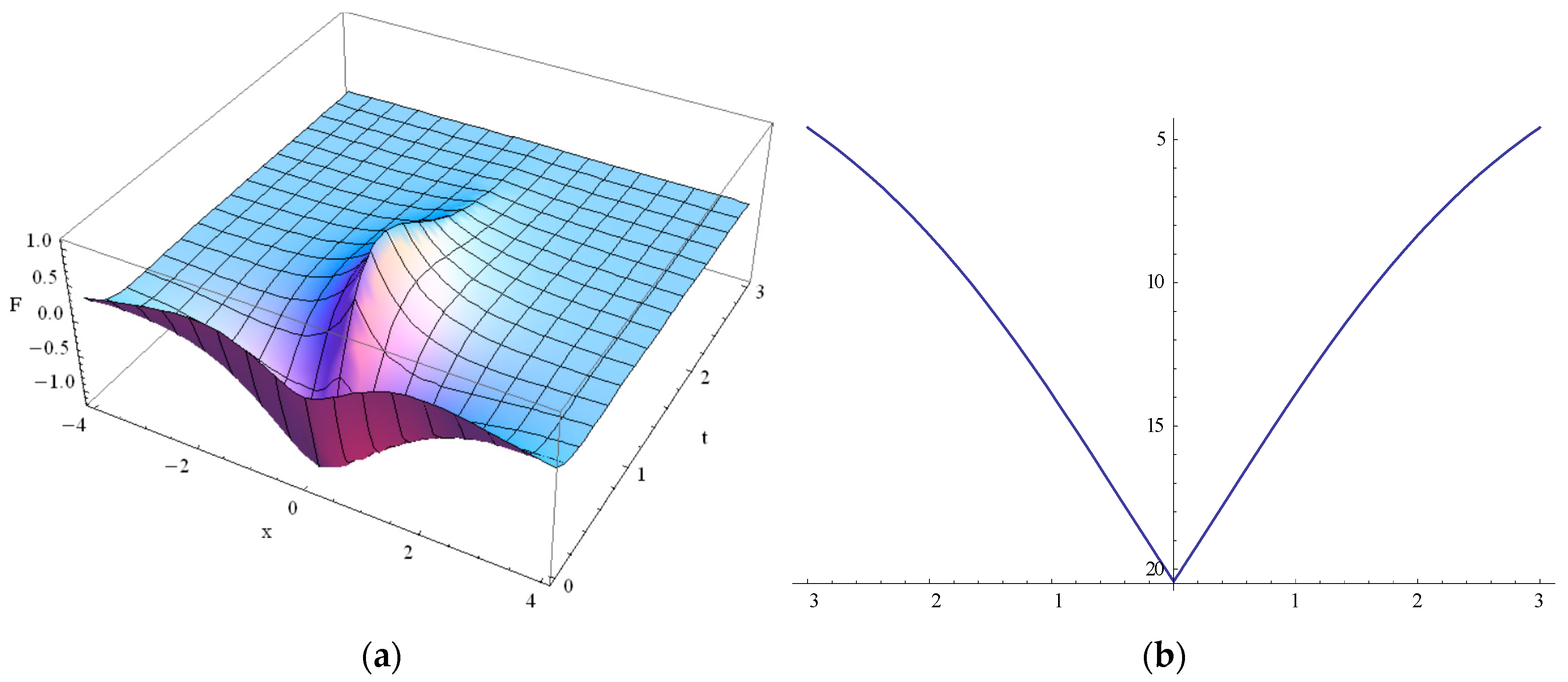
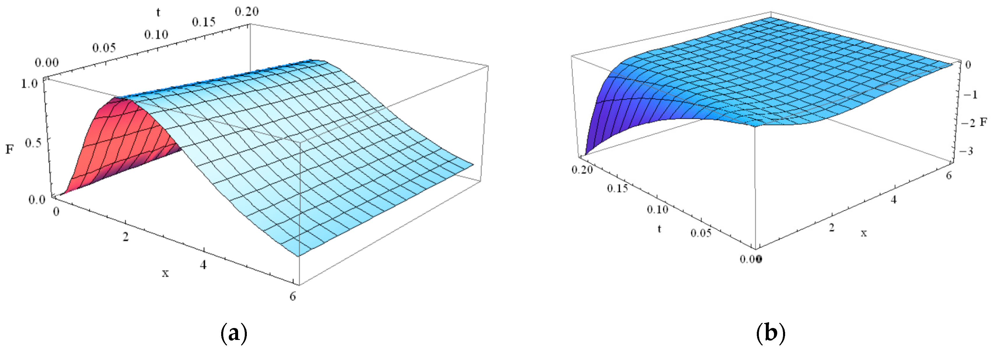
Now let us consider over diffusive regime in GK equation. The example of α = ε = 1, δ = 10 in GK type Equation (1), where its solution assumes negative values, is seen in Figure 2. The initial derivative is negative.
In this case we have slightly negative initial values of the function derivative. The behaviour of the solution completely differs from that of Fourier solution. Note, that the solution in Figure 2a assumes negative values. Moreover, observe the second branch of the solution in Figure 2b, which diverges at large times.
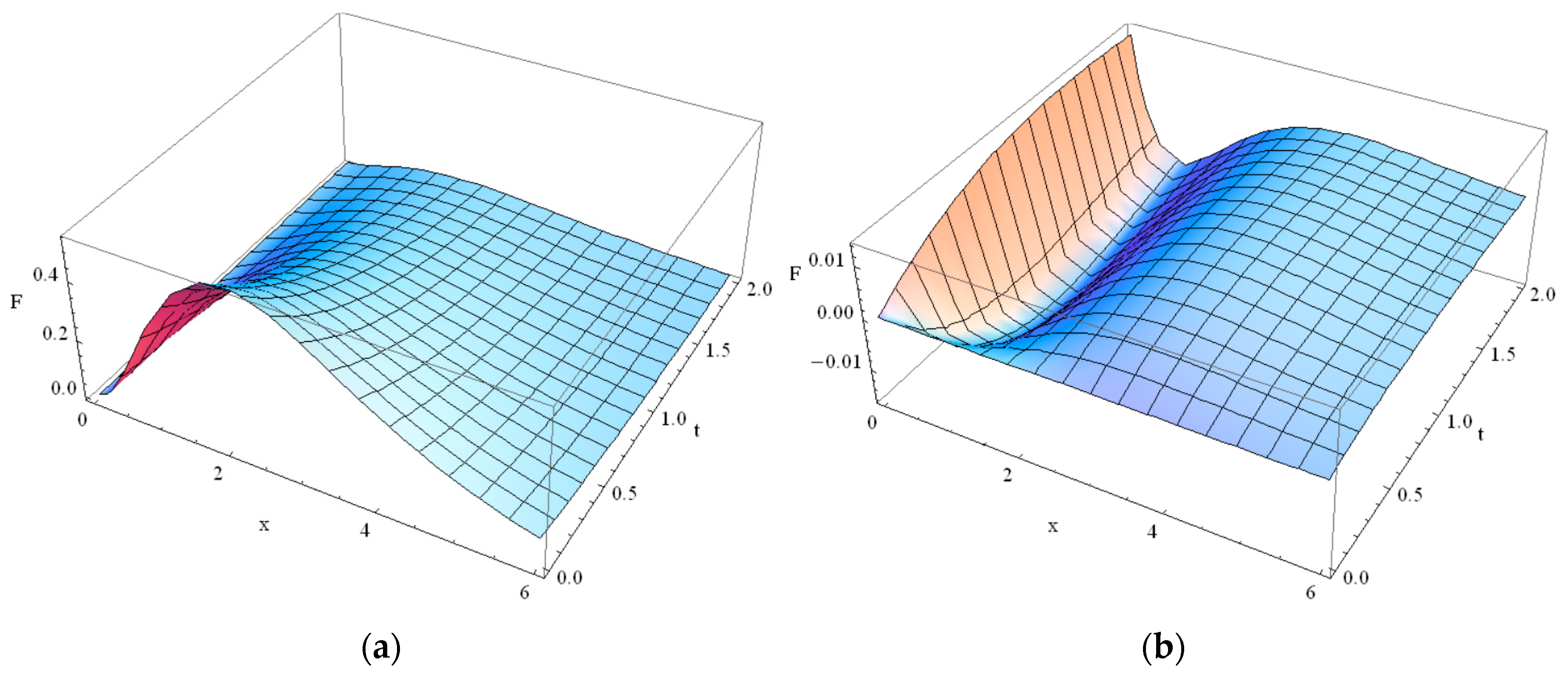
Now, consider over diffusive case α = ε = 1, δ = 10, κ = −0.5, ; the behavior of the solution is shown Figure 3a. Observe the rising solution due to the positive initial derivative (see Figure 3b with consequent fade. The solution is positive, but the maximum principle is violated since the maximum is inside the domain.
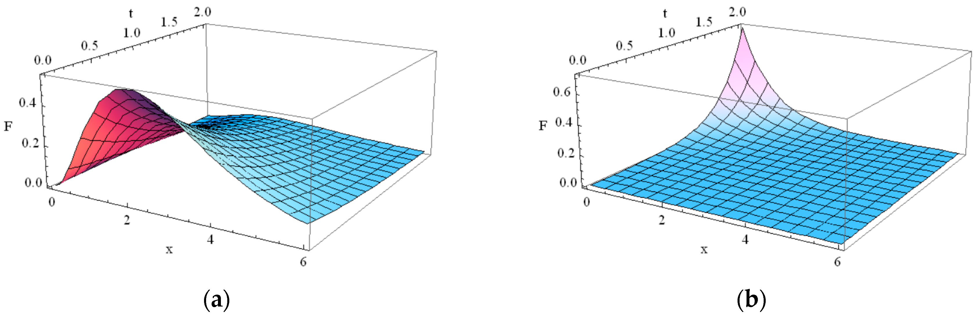
Now consider over diffusive solution in the case, when all transport contributions are of the same order, α = ε = δ = 10, κ = 1, (see Figure 4).
As seen in Figure 4 the solution first rapidly decreases due to negative sign of the initial derivative (see Figure 4b), assumes negative values and then flips back to positive and eventually relaxes to zero, as seen in Figure 4a. This behavior also does not comply with the maximum principle and non-negativity of the solution is not preserved.
Thus, we have demonstrated that over diffusive solution of GK Equation in some cases with strong negative or positive initial derivative can reach maximum or minimum inside the domain (see Figure 2 and Figure 4). Moreover, the solution (26) for can evolve from initially positive values into negative region! This occurs in over-diffusive regime for various contributions of the heat conducting mechanisms of Fourier, Cattaneo and Guyer–Krumhansl. For all comparable with each other contributions it is shown in Figure 2. For the dominating ballistic term see Figure 3 and for relatively small Cattaneo wave relaxation time see Figure 4.
5. Solution for Guyer–Krumhansl Temperature Distribution in Thin Films
Let us now consider the GK Equation, proposed for the description of the ballistic component of the temperature distribution in thin films [17]:
where is the ballistic quasi-temperature and Kn is Knudsen number, accounting for the low dimensional system. Equation (27) is the GK type Equation (1) with , , , . Not entering into the details of the physical problem of heat conduction in thin films, we just solve Equation (27) to obtain the temperature distribution with initial smooth spatial heat wave-like distribution: . Equations (19) and (23) yield two branches of the solution. For Kn = 0.1 they are slightly different from each other. It is difficult to distinguish them from each other in figures, so one of the solutions is presented in Figure 5a, the difference between the solutions is shown in Figure 5b.
For Kn = 1 the two branches of the solution behave in a different from each other way with time passing. In particular, the second branch of the solution strongly senses the initial conditions. The examples are seen in Figure 6, Figure 7 and Figure 8. Note that both negative or strongly positive solutions, violating maximum principle, may occur for Kn = 1. However, due to the fact that the solution at infinite time should eventually fade, this second branch of the solution, diverging at , seems unphysical.
The intermediate case Kn = 0.3 is shown in Figure 9. The second branch of the solution, presented in Figure 9b, exhibits waving behaviour, but it still fades out at large times. The first branch of the solution, shown in Figure 5a for Kn = 0.1, Figure 6a for Kn = 1 and in Figure 9a for Kn = 0.3, is nor sensitive to the initial conditions, neither to the values of Knudsen number. Its value varies just few percent for Kn in the range .
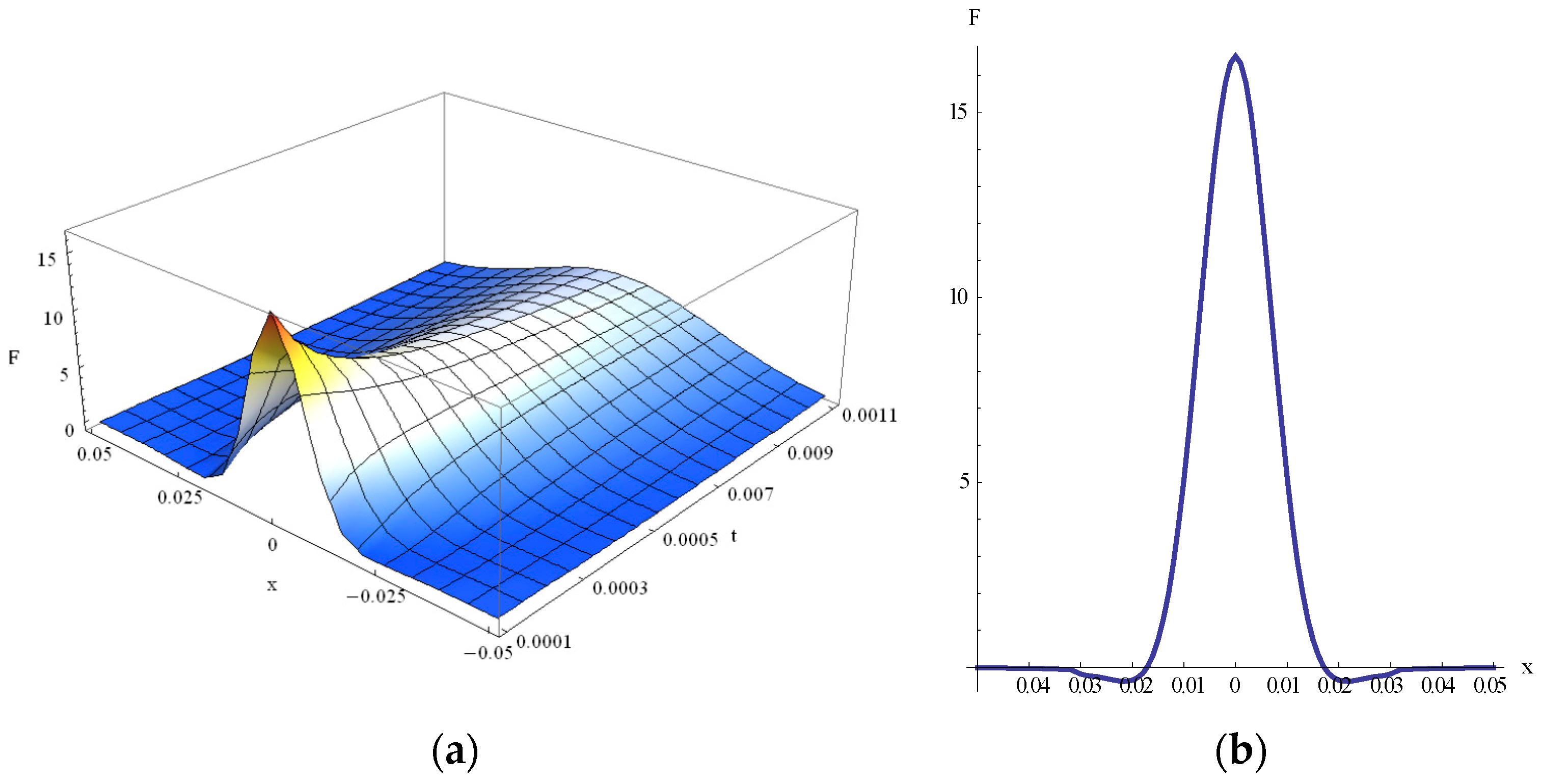
Eventually, consider the propagation of the initial Dirac δ-function. In the case of Kn = 0.3 the simplest particular solution (17) of GK Equation (1) , , when C = 1, is demonstrated in Figure 10a. The detail of the solution for t = 0.0001 is shown in Figure 10b.
We observe in Figure 10b that the solution has small negative values around the base of the evolved δ-function. It is better seen for short times; we have verified it for the range of Knudsen numbers .
6. Conclusions
With the help of the operational approach, combined with integral transforms and involving extended forms of Hermite polynomials, we have obtained exact analytical solutions for Guyer–Krumhansl type equations. The evolution of several initial functions has been studied, such as polynomial, exponential-polynomial and Dirac δ-function. The solutions were studied for the effect of Fourier heat diffusion, Cattaneo heat waves and of the ballistic heat transport.
In particular, the example of evolution of the function , its particular case was explored. The cases when Cattaneo waves or Fourier diffusion or ballistic effects dominate were explored. A small Guyer–Krumhansl term ~δ enhances thermal conduction and relaxation of the solution, counteracting the Cattaneo term ~ε; the latter describes the heat wave, which propagates at finite speed and preserves the pulse shape. In over diffusive regime, , heat transport may differ totally from Fourier. The solution may intensively grow or decrease, depending on the initial conditions, and oscillating solutions may occur. The maximum of the solution can be achieved inside the domain and neither in the initial moment, nor at the boundaries; it was demonstrated for α = ε = 1, δ = 10. Moreover, in Guyer–Krumhansl equation, in particular, in over diffusive regime the solution may temporally assume negative values, evolving from initially positive values to zero through negative region. The minimum can be reached inside the domain and the positivity is not preserved. In over diffusive regime, , for example, for α = ε = δ = 10, the solution around the initial maximum point suddenly drops below zero, then rises above zero and then relaxes to zero. Again the maximum principle and the non-negativity are not preserved. Expectably, if the Fourier heat diffusion term dominates in the equation, the solution also exhibits Fourier-like behavior and the ballistic conditions as well as the Cattaneo heat waves do not have significant effect of the solution. If all heat transport mechanisms contribute equally, minimum of the solution can nevertheless be inside the domain and the solution can turn negative, then fading to zero. Eventually, if , the Fourier solution is realized even is .
The example of the GK heat conduction in a thin film though demonstrates converging solutions for physical boundary conditions, which behave in accordance with the Second Law of thermodynamics; the maximum principle holds for non-positive initial derivative. The second branch of the solution may, however, diverge at large times, which seems unphysical. The considered examples demonstrate that in particular in over diffusive regime, dependently on the initial conditions, for strongly positive or strongly negative initial derivatives, the solution does not satisfy the maximum principle, it may become negative and may oscillate.
In forthcoming publications we will address the extension of the obtained solutions to some two- and three-dimensional cases. We will also compare and analyze the behavior of the front heat waves of the solutions to Cattaneo and to Guyer–Krumhansl Equations and include more complicated boundaries into consideration.
Acknowledgments
The author is grateful to Bingyang Cao, Laszlo I. Kiss and Yasar Demirel for fruitful discussions of physical and applied aspects of the heat transfer.
Conflicts of Interest
The author declares no conflict of interest.
References
- Fourier, J. The Analytical Theory of Heat; Cambridge University Press: London, UK, 1878. [Google Scholar]
- Onsager, L. Reciprocal Relations in irreversible processes. Phys. Rev. 1931, 37, 405. [Google Scholar] [CrossRef]
- Peshkov, V. Helium 4: The Commonwealth and International Library: Selected Readings in Physics; Elsevier: Amsterdam, The Netherlands, 2013. [Google Scholar]
- Ackerman, C.C.; Guyer, R.A. Temperature pulses in dielectric solids. Ann. Phys. 1968, 50, 128–185. [Google Scholar] [CrossRef]
- Ackerman, C.C.; Overton, W.C. Second sound in solid helium-3. Phys. Rev. Lett. 1969, 22, 764. [Google Scholar] [CrossRef]
- McNelly, T.F.; Rogers, S.J.; Channin, D.J.; Rollefson, R.; Goubau, W.M.; Schmidt, G.E.; Krumhansl, J.A.; Pohl, R.O. Heat pulses in NaF: Onset of second sound. Phys. Rev. Lett. 1970, 24, 100. [Google Scholar] [CrossRef]
- Narayanamurti, V.; Dynes, R.D. Observation of second sound in Bismuth. Phys. Rev. Lett. 1972, 26, 1461–1465. [Google Scholar] [CrossRef]
- Cattaneo, C. Sur une forme de l’équation de la chaleur éliminant le paradoxe d’une propagation instantanée. Compt. Rendu. 1958, 247, 431–433. [Google Scholar]
- Cattaneo, C. Sulla conduzione del calore. Atti Sem. Mat. Fis. Univ. Modena 1948, 3, 83–101. [Google Scholar]
- Bright, T.J.; Zhang, Z.M. Common misperceptions of the hyperbolic heat equation. J. Thermophys. Heat Transf. 2009, 23, 601–607. [Google Scholar] [CrossRef]
- Shiomi, J.; Maruyama, S. Non-Fourier heat conduction in a single-walled carbon nanotube: Classical molecular dynamics simulations. Phys. Rev. B 2006, 73, 205420. [Google Scholar] [CrossRef]
- Bai, C.; Lavine, A.S. On hyperbolic heat conduction and the second law of thermodynamics. J. Heat Transf. 1995, 117, 256–263. [Google Scholar] [CrossRef]
- Porrà, J.M.; Masoliver, J.; Weiss, G.H. When the telegrapher’s Equation furnishes a better approximation to the transport Equation than the diffusion approximation. Phys. Rev. E 1997, 55, 7771–7774. [Google Scholar] [CrossRef]
- Körner, C.; Bergmann, H.W. The physical defects of the hyperbolic heat conduction equation. Appl. Phys. A 1998, 67, 397–401. [Google Scholar] [CrossRef]
- Guyer, R.A.; Krumhansl, J.A. Thermal conductivity, second sound and phonon hydrodynamic phenomena in non-metallic crystals. Phys. Rev. 1966, 148, 778–788. [Google Scholar] [CrossRef]
- Guyer, R.A.; Krumhansl, J.A. Solution of the linearized phonon Boltzmann equation. Phys. Rev. 1966, 148, 766–778. [Google Scholar] [CrossRef]
- Lebon, G.; Machrafi, H.; Gremela, M.; Dubois, C. An extended thermodynamic model of transient heat conduction at sub-continuum scales. Proc. R. Soc. A 2011, 467, 3241–3256. [Google Scholar] [CrossRef]
- Minnich, J.; Johnson, J.A.; Schmidt, A.J.; Esfarjani, K.; Dresselhaus, M.S.; Nelson, K.A.; Chen, G. Thermal conductivity spectroscopy technique to measure phonon mean free paths. Phys. Rev. Lett. 2011, 107, 095901. [Google Scholar] [CrossRef] [PubMed]
- Casimir, H.B.G. Note on the Conduction of Heat in Crystals. Physica 1938, 5, 495–500. [Google Scholar] [CrossRef]
- Baringhaus, J.; Ruan, M.; Edler, F.; Tejeda, A.; Sicot, M.; Ibrahimi, A.T.; Jiang, Z.; Conrad, E.; Berger, C.; Tegenkamp, C.; et al. Exceptional ballistic transport in epitaxial graphene nanoribbons. Nature 2014, 506, 349–354. [Google Scholar] [CrossRef] [PubMed]
- Hochbaum, A.I.; Chen, R.; Delgado, R.D.; Liang, W.; Garnett, E.C.; Najarian, M.; Majumdar, A.; Yang, P. Enhanced thermoelectric performance of rough silicon nanowires. Nature 2008, 451, 163–167. [Google Scholar] [CrossRef] [PubMed]
- Boukai, A.I.; Bunimovich, Y.; Tahir-Kheli, J.; Yu, J.-K.; Goddard, W.A.; Heath, J.R. Silicon nanowires as efficient thermoelectric materials. Nature 2008, 451, 168. [Google Scholar] [CrossRef] [PubMed]
- Paddock, C.A.; Eesley, G.L. Transient thermoreflectance from thin metal films. J. Appl. Phys. 1986, 60, 285. [Google Scholar] [CrossRef]
- Maldovan, M. Transition between ballistic and diffusive heat transport regimes in silicon materials. Appl. Phys. Lett. 2012, 101, 113110. [Google Scholar] [CrossRef]
- Cahill, D.G. Thermal conductivity measurement from 30 to 750 K: The 3ω method. Rev. Sci. Instrum. 1990, 61, 802–808. [Google Scholar] [CrossRef]
- Van, P.; Berezovski, A.; Fulop, T.; Grof, G.; Kovacs, R.; Lovas, A.; Verhas, J. Guyer-Krumhansl-type heat conduction at room temperature. arXiv, 2017; arXiv:arXiv:1704.00341. [Google Scholar]
- Tang, D.W.; Araki, N. Non-Fourier heat conduction behaviour in finite mediums under pulse surface heating. Mater. Sci. Eng. 2000, 292, 173–178. [Google Scholar] [CrossRef]
- Kaminski, W. Hyperbolic heat conduction Equations for materials with a nonhomogeneous inner structure. J. Heat Transf. 1990, 112, 555–560. [Google Scholar] [CrossRef]
- Mitra, K.; Kumar, S.; Vedavarz, A.; Moallemi, M.K. Experimental evidence of hyperbolic heat conduction in processed meat. J. Heat Transf. 1995, 117, 568–573. [Google Scholar] [CrossRef]
- Herwig, H.; Beckert, K. Fourier versus non-Fourier heat conduction in materials with a nonhomogeneous inner structure. J. Heat Transf. 2000, 122, 363–365. [Google Scholar] [CrossRef]
- Roetzel, W.; Putra, N.; Das, S.K. Experiment and analysis for non-Fourier conduction in materials with non-homogeneous inner structure. Int. J. Therm. Sci. 2003, 42, 541–552. [Google Scholar] [CrossRef]
- Scott, E.P.; Tilahun, M.; Vick, B. The question of thermal waves in heterogeneous and biological materials. J. Biomech. Eng. 2009, 131, 074518. [Google Scholar] [CrossRef] [PubMed]
- Chen, G. Ballistic-Diffusive Heat-Conduction equations. Phys. Rev. Lett. 2001, 86, 2297–2300. [Google Scholar] [CrossRef] [PubMed]
- Hsiao, T.; Chang, H.; Liou, S.; Chu, M.; Lee, S.; Chang, C. Observation of room-temperature ballistic thermal conduction persisting over 8.3 mm in SiGe nanowires. Nat. Nanotechnol. 2013, 8, 534–538. [Google Scholar] [CrossRef] [PubMed]
- Zhang, Y.; Ye, W. Modified ballistic–diffusive equations for transient non-continuum heat conduction. Int. J. Heat Mass Transf. 2015, 83, 51–63. [Google Scholar] [CrossRef]
- Kovacs, R.; Van, P. Generalized heat conduction in heat pulse experiments. Int. J. Heat Mass Transf. 2015, 83, 613–620. [Google Scholar] [CrossRef]
- Van, P.; Fulop, T. Universality in heat conduction theory: Weakly non-local thermodynamics. Ann. Phys. 2012, 524, 470–478. [Google Scholar] [CrossRef]
- Dattoli, G.; Srivastava, H.M.; Zhukovsky, K.V. Operational methods and Differential equations with Applications to Initial-Value problems. Appl. Math. Comput. 2007, 184, 979–1001. [Google Scholar] [CrossRef]
- Zhukovsky, K. Solution of Some Types of Differential equations: Operational Calculus and Inverse Differential Operators. Sci. World J. 2014, 2014, 1–8. [Google Scholar] [CrossRef] [PubMed]
- Zhukovsky, K.V. A method of inverse differential operators using ortogonal polynomials and special functions for solving some types of differential equations and physical problems. Mosc. Univ. Phys. Bull. 2015, 70, 93–100. [Google Scholar] [CrossRef]
- Dattoli, G.; Srivastava, H.M.; Zhukovsky, K. A new family of integral transforms and their applications. Integral Transform. Spec. Funct. 2006, 17, 31–37. [Google Scholar] [CrossRef]
- Srivastava, H.M.; Manocha, H.L. A Treatise on Generating Functions; John Wiley and Sons: New York, NY, USA, 1984. [Google Scholar]
- Sokolov, A.A.; Ternov, I.M.; Zhukovsky, V.C.; Borisov, A.V. Gauge Fields (Kalibrovochnye Polya); Moscow State University: Moscow, Russia, 1986; p. 264. (In Russian) [Google Scholar]
- Zhukovsky, K.V. Operational solution for some types of second order differential equations and for relevant physical problems. J. Math. Anal. Appl. 2017, 446, 628–647. [Google Scholar] [CrossRef]
- Zhukovsky, K.V. Operational method of solution of linear non-integer ordinary and partial differential equations. Springer Plus 2016, 5, 119. [Google Scholar] [CrossRef] [PubMed]
- Srivastava, H.M.; Zhukovsky, K.V. Solutions of some types of differential equations and of their associated physical problems by means of inverse differential operators. In Mathematical Analysis, Approximation Theory and Their Applications; Springer Optimization and Its Applications Series; Rassias, H.M., Gupta, V., Eds.; Springer International Publishing: Cham, Switzerland, 2016; Volume 111, pp. 573–629. [Google Scholar]
- Zhukovsky, K.V. Operational solution of differential equations with derivatives of non-integer order, Black–Scholes type and heat conduction. Mosc. Univ. Phys. Bull. 2016, 71, 3237–3244. [Google Scholar] [CrossRef]
- Zhukovsky, K.V. Solving evolutionary-type differential equations and physical problems using the operator method. Theor. Math. Phys. 2017, 190, 52–68. [Google Scholar] [CrossRef]
- De Jagher, P.C. A hyperbolic “diffusion equation” taking a finite collision frequency into account. Physica A 1980, 101, 629–633. [Google Scholar] [CrossRef]
- Zhukovsky, K.V. Exact solution of Guyer-Krumhansl type heat Equation by operational method. Int. J. Heat Mass Transf. 2016, 96, 132–144. [Google Scholar] [CrossRef]
- Parker, W.J.; Jenkins, R.J.; Butler, C.P.; Abbott, G.L. Flash method of determining thermal diffusivity, heat capacity, and thermal conductivity. J. Appl. Phys. 1961, 32, 1679–1684. [Google Scholar] [CrossRef]
- Zhukovsky, K.V.; Srivastava, H.M. Analytical solutions for heat diffusion beyond Fourier law. Appl. Math. Comput. 2017, 293, 423–437. [Google Scholar] [CrossRef]
- Zhukovsky, K. Operational approach and solutions of hyperbolic heat conduction equations. Axioms 2016, 5, 28. [Google Scholar] [CrossRef]
- Dattoli, G.; Górska, K.; Horzela, A.; Penson, K.A.; Sabia, E. Theory of relativistic heat polynomials and one-sided Lévy distributions. J. Math. Phys. 2017, 58, 063510. [Google Scholar] [CrossRef]
- Dattoli, G.; Srivastava, H.M.; Zhukovsky, K. Оrthogonality properties of the Hermite and related polynomials. J. Comput. Appl. Math. 2005, 182, 165–172. [Google Scholar] [CrossRef]
- Gould, H.W.; Hopper, A.T. Operational formulas connected with two generalizations of Hermite polynomials. Duke Math. J. 1962, 29, 51–63. [Google Scholar] [CrossRef]
- Zhukovsky, K.V. Violation of the maximum principle and negative solutions with pulse propagation in Guyer–Krumhansl model. Int. J. Heat Mass Transf. 2016, 98, 523–529. [Google Scholar] [CrossRef]
Figure 1.
(a) Fourier-like solution of GK type Equation (1) for , α = ε = δ = 1, κ = −0.5; (b) The initial derivative, .
Figure 1.
(a) Fourier-like solution of GK type Equation (1) for , α = ε = δ = 1, κ = −0.5; (b) The initial derivative, .
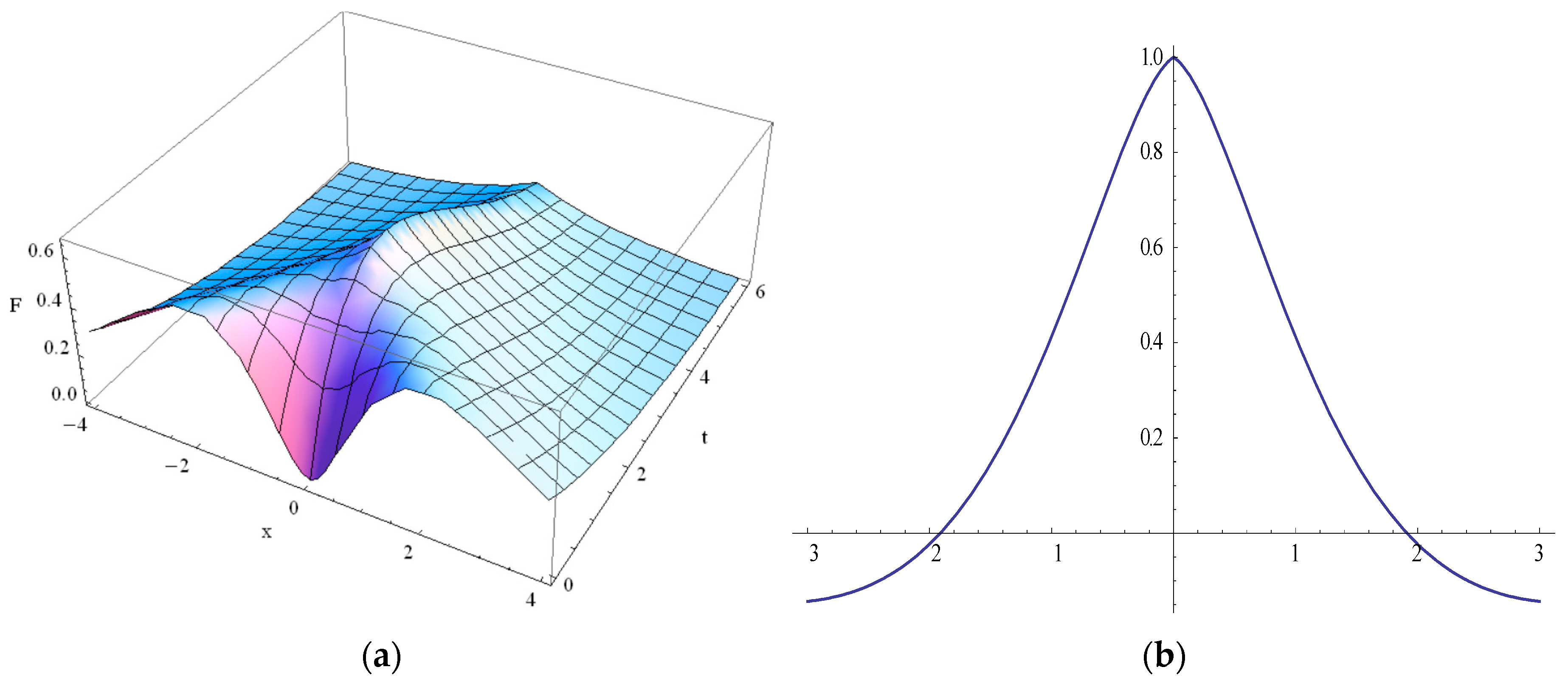
Figure 2.
Over diffusive solutions of GK Equation (1) for dominating ballistic contribution: α = ε = 1, δ = 10, κ = 0.5 for ; (a) Converging solution; (b) Diverging at solution.
Figure 2.
Over diffusive solutions of GK Equation (1) for dominating ballistic contribution: α = ε = 1, δ = 10, κ = 0.5 for ; (a) Converging solution; (b) Diverging at solution.
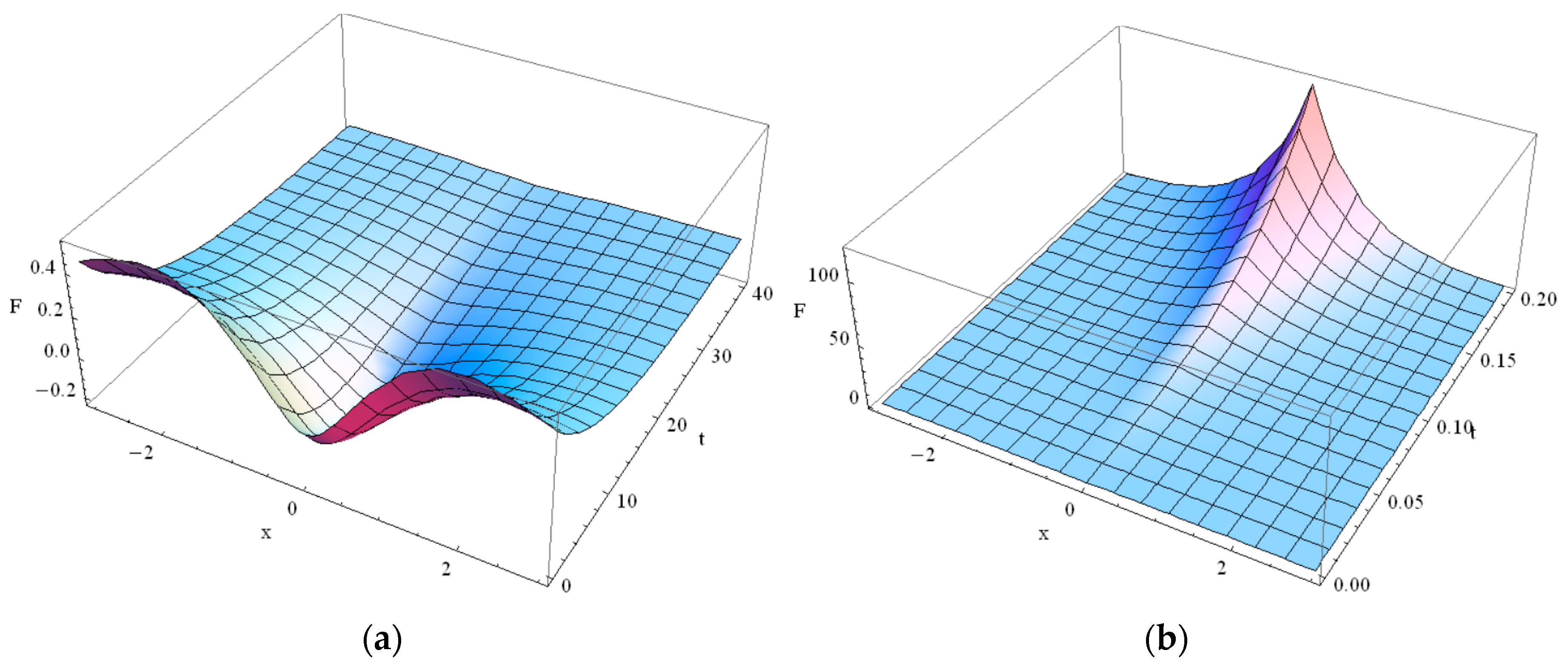
Figure 3.
Over diffusive solution of GK type Equation (1) for dominating contribution of the ballistic effects: α = ε = 1, δ = 10, κ = −0.5, (a) the solution for ; (b) The initial derivative .
Figure 3.
Over diffusive solution of GK type Equation (1) for dominating contribution of the ballistic effects: α = ε = 1, δ = 10, κ = −0.5, (a) the solution for ; (b) The initial derivative .

Figure 4.
The over diffusive solution of GK Equation (1) for small Cattaneo term, α = ε = δ = 10, κ = 1, (a) the solution for ; (b) The initial derivative .
Figure 4.
The over diffusive solution of GK Equation (1) for small Cattaneo term, α = ε = δ = 10, κ = 1, (a) the solution for ; (b) The initial derivative .

Figure 5.
Initial heat distribution evolution in one-dimensional film with Knudsen number Kn = 0.1. (a) One solution; (b) The difference between two solutions.
Figure 5.
Initial heat distribution evolution in one-dimensional film with Knudsen number Kn = 0.1. (a) One solution; (b) The difference between two solutions.

Figure 6.
Evolution of the initial heat distribution in one-dimensional film with Knudsen number Kn = 1, . (a) One solution; (b) The second solution.
Figure 6.
Evolution of the initial heat distribution in one-dimensional film with Knudsen number Kn = 1, . (a) One solution; (b) The second solution.

Figure 7.
Evolution of the second solution for initial heat distribution in one-dimensional film with Knudsen number Kn = 1, (a) The case of : (b)The case of .
Figure 7.
Evolution of the second solution for initial heat distribution in one-dimensional film with Knudsen number Kn = 1, (a) The case of : (b)The case of .

Figure 8.
Evolution of the initial heat distribution in one-dimensional film with Knudsen number Kn = 1, . (a) One solution; (b) The second solution.
Figure 8.
Evolution of the initial heat distribution in one-dimensional film with Knudsen number Kn = 1, . (a) One solution; (b) The second solution.

Figure 9.
Initial heat distribution evolution in one-dimensional film with Knudsen number Kn = 0.3. (a) One solution; (b) The other solution.
Figure 9.
Initial heat distribution evolution in one-dimensional film with Knudsen number Kn = 0.3. (a) One solution; (b) The other solution.
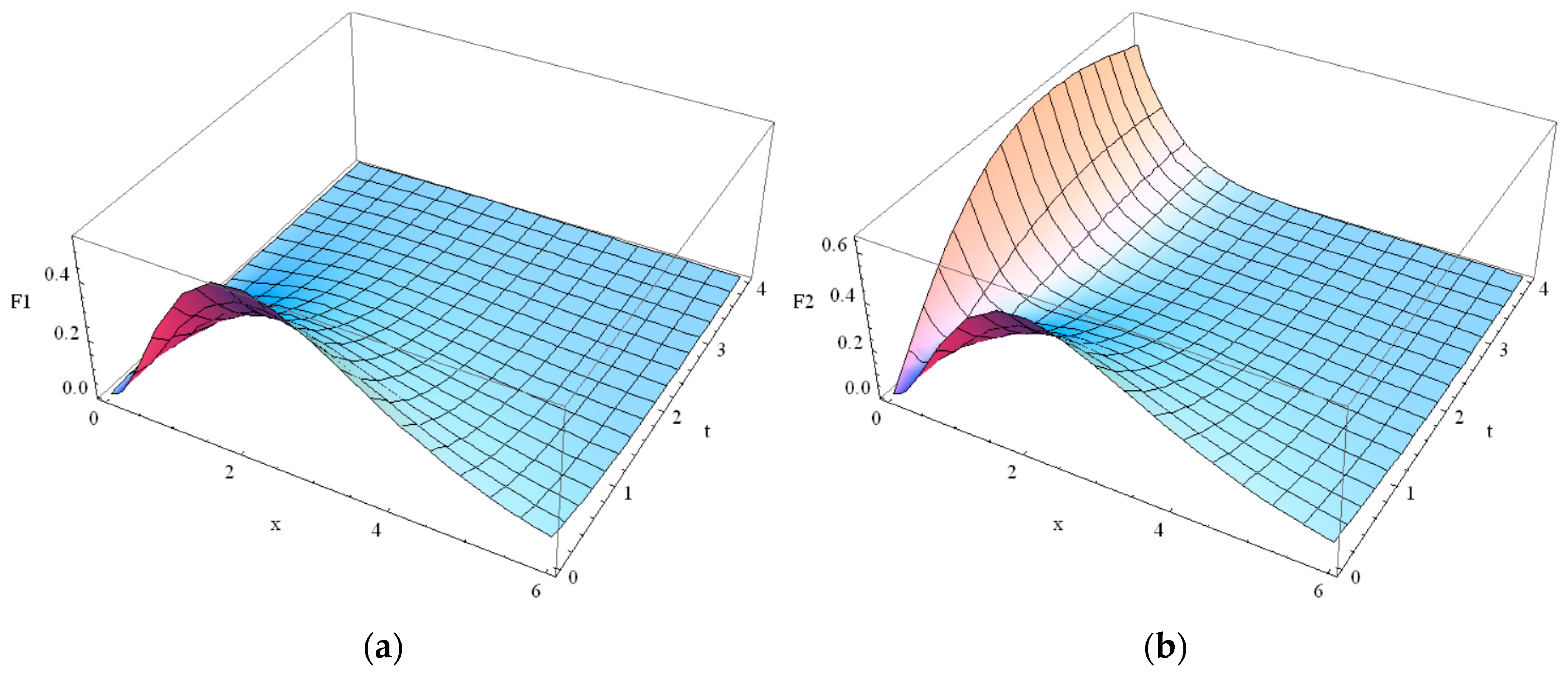
Figure 10.
(a) The example of the particular solution of GK type Equation (1) for Kn = 0.3, , ; (b) The detail of the solution for t = 0.0001.
Figure 10.
(a) The example of the particular solution of GK type Equation (1) for Kn = 0.3, , ; (b) The detail of the solution for t = 0.0001.
© 2017 by the author. Licensee MDPI, Basel, Switzerland. This article is an open access article distributed under the terms and conditions of the Creative Commons Attribution (CC BY) license (http://creativecommons.org/licenses/by/4.0/).
Share and Cite
MDPI and ACS Style
Zhukovsky, K. Exact Negative Solutions for Guyer–Krumhansl Type Equation and the Maximum Principle Violation. Entropy 2017, 19, 440. https://doi.org/10.3390/e19090440
AMA Style
Zhukovsky K. Exact Negative Solutions for Guyer–Krumhansl Type Equation and the Maximum Principle Violation. Entropy. 2017; 19(9):440. https://doi.org/10.3390/e19090440
Chicago/Turabian StyleZhukovsky, Konstantin. 2017. "Exact Negative Solutions for Guyer–Krumhansl Type Equation and the Maximum Principle Violation" Entropy 19, no. 9: 440. https://doi.org/10.3390/e19090440
Note that from the first issue of 2016, this journal uses article numbers instead of page numbers. See further details here.