Maximum Likelihood-Based Iterated Divided Difference Filter for Nonlinear Systems from Discrete Noisy Measurements

Abstract
: A new filter named the maximum likelihood-based iterated divided difference filter (MLIDDF) is developed to improve the low state estimation accuracy of nonlinear state estimation due to large initial estimation errors and nonlinearity of measurement equations. The MLIDDF algorithm is derivative-free and implemented only by calculating the functional evaluations. The MLIDDF algorithm involves the use of the iteration measurement update and the current measurement, and the iteration termination criterion based on maximum likelihood is introduced in the measurement update step, so the MLIDDF is guaranteed to produce a sequence estimate that moves up the maximum likelihood surface. In a simulation, its performance is compared against that of the unscented Kalman filter (UKF), divided difference filter (DDF), iterated unscented Kalman filter (IUKF) and iterated divided difference filter (IDDF) both using a traditional iteration strategy. Simulation results demonstrate that the accumulated mean-square root error for the MLIDDF algorithm in position is reduced by 63% compared to that of UKF and DDF algorithms, and by 7% compared to that of IUKF and IDDF algorithms. The new algorithm thus has better state estimation accuracy and a fast convergence rate.1. Introduction
The problem of estimating the state of a nonlinear stochastic system from noisy measurement data has been the subject of considerable research interest during the past few years. Up to now the extended Kalman filter (EKF) has unquestionably been the dominating state estimation technique [1,2]. The EKF linearizes both the nonlinear process and the measurement dynamics with a first-order Taylor series expansion about the current state estimate. However, its accuracy depends heavily on the severity of nonlinearities. The EKF may introduce large errors and even give a divergent estimate when the nonlinearities become severe [3,4]. To improve the estimation accuracy, the second-order EKF proposed retains the Taylor series expansion up to the second term. The second–order EKF generally improves estimation accuracy, but at the expense of an increased computational burden [5]. Another attempt to improve the performance of the EKF involves the use of an iterative measurement update; the resulting algorithm is called the Iterated Extended Kalman filter (IEKF) [6]. The basic idea of IEKF is to linearize the measurement model around the updated state rather than the predicted state. This is achieved iteratively, and it involves the use of the current measurement. The IEKF has been proven to be more accurate on the condition that the state estimate is close enough to the true value, however, this is rarely the case in practice [7]. It was pointed out in [8] that the sequence of iterations generated by the IEKF and that generated by the Gauss-Newton method were identical, thus globally convergence was guaranteed. However, the Gauss-Newton method does not ensure that it goes up the likelihood surface [9,10]. Furthermore, EKF and IEKF require Jacobians, and the second-order KF requires Jacobians and Hessians. Calculation of Jacobians and Hessians is often numerically unstable and computationally intensive. In some system, the Jacobians and Hessians do not exit, which limits the applications of EKF, second-order EKF and IEKF.
Recently, there has been development in derivative-free state estimators. The finite difference has been used in the Kalman filter framework and the resulting filter is referred to as the finite difference filter (FDF) [11]. The FDF uses the first-order difference to approximate the derivative of the nonlinear function; it may introduce large state estimation errors due to a high nonlinearity, similar to the EKF. The unscented Kalman filter (UKF) proposed in [12,13] uses a minimal set of deterministically chosen sample points to capture the mean and covariance of a Gaussian density. When propagated through a nonlinear function, these points capture the true mean and covariance up to a second-order of the nonlinear function. However, the parameters used in the UKF are required to tune finely in order to prevent the propagation of non-positive definite covariance matrix for a state vector's dimension higher than three. Another Gaussian filter, named the divided difference filter (DDF) was introduced in [14] using multidimensional Stirling's interpolation formula. It is shown in [15] that the UKF and DDF algorithms are commonly referred to as sigma point filters due to the properties of deterministic sampling and weighted statistical estimation [16], but the covariance obtained in the DDF is more accurate than that in the UKF. The iterated UKF with the variable step (IUKF-VS) in [10] proposed improved the accuracy of state estimation but its runtime was large due to its computation of the sigma points. Lastly, a relatively new technique called the particle filter (PF) uses a set of randomly chosen samples with associated weights to approximate the posterior density [17] and its variants are presented in [18]. The large number of samples required often makes the use of PF computationally expensive, and the performance of PF is crucially dependent on the selection of the proposal distribution. Table 1 lists the pro and cons of the above filters.
The DDF also shows its weakness in the state estimation due to the large initial error and high nonlinearity in the application for state estimation of maneuvering target in the air-traffic control and ballistic re-entry target. Emboldened by the superiority of DDF, the basic idea of the IEKF and the iteration termination condition based on maximum likelihood, we propose a new filter named the maximum likelihood based iterated divided difference Kalman filter (MLIDDF). The performance of the state estimation for MLIDDF is greatly improved when involving the use of the iteration measurement update in the MLIDDF and the use of the current measurement. The remainder of this paper is organized as follows: in Section 2, we develop the maximum likelihood surface based iterated divided difference Kalman filter (MLIDDF). Section 3 presents the applications of the MLIDDF to state estimation for maneuvering targets in air-traffic control and ballistic target re-entry applications and discuss the simulation results. Finally, Section 4 concludes the paper and presents our outlook on future work.
2. Development of Likelihood Surface Based Iterated Divided Difference Filter
2.1. Divided Difference Filter
Consider the nonlinear function:
Assuming that the random variable x ∈ ℝnx has Gaussian density with mean x̄ and covariance Px. The following linear transformation of x is introduced:
The transformation matrix Sx is selected as a square Cholesky factor of the covariance matrix Px such that , so the elements of z become mutually uncorrelated [14]. And the function f̃ is defined by:
The multidimensional Stirling interpolation formula of Equation (3) about z̄ up to second-order terms is given by:
The divided difference operators D̃Δzf̃, are defined as:
The partial operators μ and δ are defined as:
We can obtain the approximate mean, covariance and cross-covariance of y using Equation (4):
Consider the state estimation problem of a nonlinear dynamics system with additive noise, the nx-dimensional state vector xk of the system evolves according to the nonlinear stochastic difference equation:
 (0, Qk−1), vk ∼
(0, Rk).
(0, Qk−1), vk ∼
(0, Rk).Suppose the state distribution at k-1 time instant is xk−1∼
(x̂k−1, Pk−1), and a square Cholesky factor of Pk−1 is Ŝx,k−1. The divided difference filter (DDF) obtained with Equations (9)–(11) can be described as follows:
Step 1. Time update
Calculate matrices containing the first- and second- divided difference on the estimated state x̂k−1 at k-1 time:
Evaluate the predicted state and square root of corresponding covariance:
ŝx,j is j-th column of Ŝx,k−1. Tria() is denoted as a general triagularization algorithm and Sw,k−1 denotes a square-root factor of Qk−1 such that .
Step 2. Measurement update
Calculate matrices containing the first- and second-divided difference on the predicted state x̄k:
where s̄x,j is the j-th column of S̄x,k.Evaluate the predicted measurement, square root of innovation covariance and cross-covariance:
here Sv,k denotes a square root of Rk such that .Evaluate the gain, state estimation and square root of corresponding covariance at k time:
here, the symbol “/” represents the matrix right divide operator.
2.2. Refining the Measurement Update Based on Divided Difference
Consider x̄k and current measurement zk as realization of independent random vectors with multivariate normal distributions, e.g., x̄k ∼
(xk, P̄k) and zk ∼
(h(xk), Rk). For convenience, the two vectors are formed to a single augmented one Z = [zk x̄k]T. According to the independent assumption, we have:
Here:
The update measurement problem becomes the one that computing the optimal state estimation and corresponding covariance given Z, g and Q̃.
Defining the objective function:
Assuming the i-iterate is , we can obtain the following equation [8]:
We know the sequence of iterates generated by the IEKF and that generated by the Gauss-Newton method were identical, thus globally convergent was guaranteed. The initial state x̄k is included in the measurement update, the value of x̄k has a direct and large effect on the final state estimation. When the measurement model fully observes the state, the estimated state is more approximate to the true state than the predicted state x̄k [7]. Substituting x̄k by into Equation (29), hence, the following iterative formula is obtained:
Compared to Equation (29), the Equation (30) is simpler, and the two equations are identical when there is a single iteration.
Now we consider the gain:
The terms of Equations (32) and (33) are achieved by expanding the measurement Equation (13) up to a first-order Taylor term so that the linearized error is introduced due to the high-order truncated terms. As for the highly nonlinear measurement equation, the accuracy for state estimation is decreased if the linearized error is only propagated in the Equation (30). To decrease the propagated error, we can recalculate Equations (18)–(22) to obtain the terms , in the following way:
Hence, we can obtain the following iterative formula:
2.3. Maximum Likelihood Based Iteration Termination Criterion
In the measurement update step of the IEKF algorithm, the inequality is used as the criterion to terminate the iteration procedure, where ε is the predetermined threshold. The threshold ε is crucial to successfully using the IEKF algorithm, but selecting a proper value of ε is difficult [10]. The sequence of iterations generated according to the above termination condition has the property of global convergence; however, it is not guaranteed to move up the likelihood surface, so an iteration termination criterion based on maximum likelihood surface is introduced.
Consider
and zk as the realization of independent random vectors with multivariate normal distributions, i.e.,
, zk ∼
(h(xk),Rk). The likelihood function of the two vectors xk and zk is defined as:
Meanwhile, the likelihood surface is defined as follows:
We know that the solution that maximizes the likelihood function is equivalent to minimizing the cost function J(xk). The optimal value of J(xk) is difficult to obtain, but the following inequality holds:
We say that is close to the maximum likelihood surface than , equivalently, has a more accurate approximation than to the minimum value of J(xk) [10]. Extending Equation (42) and using , we immediately obtain the following inequality:
The sequence generated is guaranteed to go up the likelihood surface using Equation (43) as the criterion to iteration termination.
2.4. Maximum Likelihood Based Iterated Divided Difference Filter
We have now arrived at the central issue of this paper, namely, the maximum likelihood based iterated divided difference filter. Enlightened by the development of IEKF and the superiority of DDF, we can derive the maximum likelihood based iterated divided difference filter (MLIDDF) which involves the use of the iteration measurement update and the current measurement. But in view of the potential problems exhibited by the IEKF, we shall refine the covariance and cross-covariance based on divided difference and use the termination criterion which guarantees the sequence obtained moves up the maximum likelihood surface. The MLIDDF is described as follows:
Step 1. Time update
Evaluate the predicted state x̄k and square Cholesky factor S̄k of the corresponding covariance P̄k using the Equations (14)–(17).
Step 2. Measurement update
Let and . Suppose that the i-th iterates are and .
Evaluate the first- and second-order difference matrices using Equation (34) and (35).
Evaluate the square root of innovation covariance and cross-covariance:
Evaluate the gain:
Evaluate the state and the square root of corresponding covariance:
where is the j-th column of .
Step 3. If the following inequality holds:
The iteration returns to Step 2; otherwise continue to Step 4. , are defined in the Equations (44) and (45).
Step 4. If the inequality is not satisfied or if i is too large (i > Nmax), and the ultimate state estimation and square root of corresponding covariance at k time instant are:
The MLIDDF algorithm has the virtues of free-derivative and better numerical stability. The measurement update of MLIDDF algorithm is transformed to a nonlinear least-square problem; the optimum state estimation and covariance are solved using Gauss-Newton method, so the MLIDDF algorithm has the same global convergence as the Gauss-Newton method. Moreover, the iteration termination condition that makes the sequence move up the maximum likelihood surface is used in the measurement update process.
3. Simulation and Analysis
In this section, we reported the experimental results obtained by applying the MLIDDF to the nonlinear state estimation of a maneuvering target in an air-traffic control scenario and a ballistic target re-entry scenario. To demonstrate the performance of the MLIDDF algorithm we compared its performance against the UKF, DDF, and the iterated UKF (IUKF) and iterated DDF (IDDF), both using a traditional iteration strategy.
3.1. Maneuvering Target Tracking in the Air-Traffic Control Scenario
We consider a typical air-traffic control scenario, where an aircraft executes a maneuvering turn in a horizontal plane at a constant, but unknown turn rate Ω. The kinematics of the turning motion can be modeled by the following nonlinear process equation [2,19]:
The process nose wk−1∼
(0, Q) with a nonsingular covariance:
The parameters q1 and q2 are related to process noise intensities. A radar is fixed at the origin of the place and equipped to measure the range, r and bearing, θ. Hence, the measurement equation is written:
(0, R) and
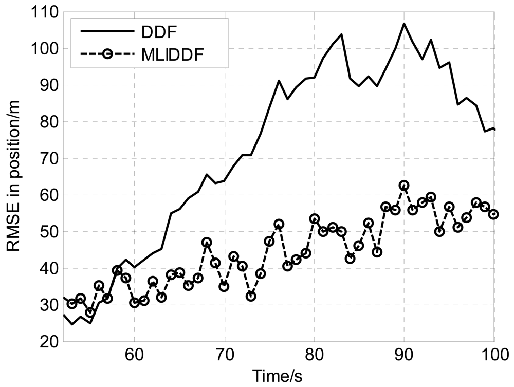
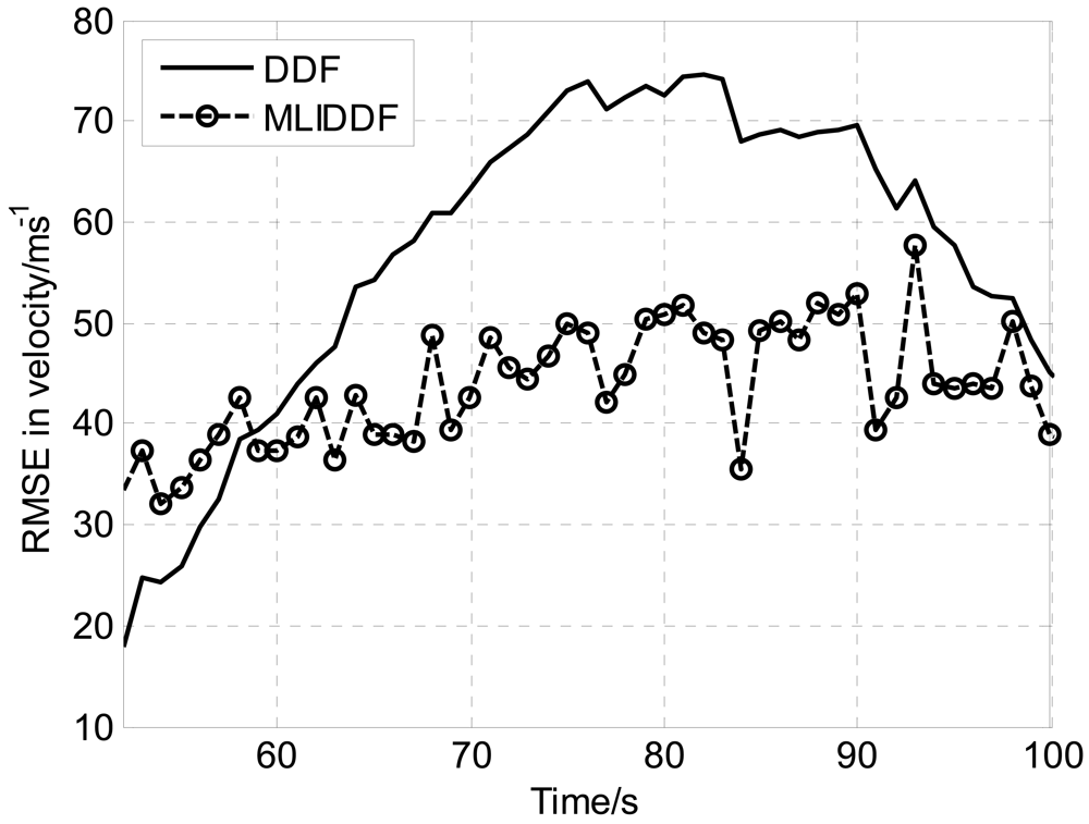
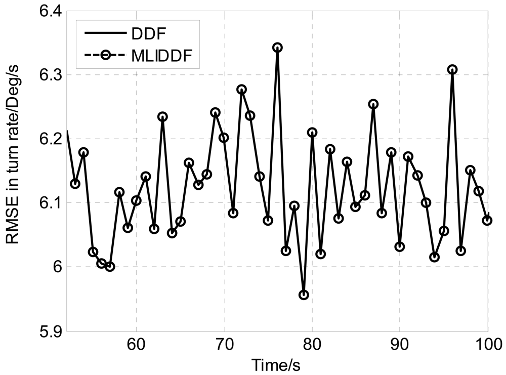
.The parameters used in this simulation were the same as those in [19]. To tracking the maneuvering aircraft we use the proposed MLIDDF algorithm and compare its performance against the DDF. We use the root-mean square error (RMSE) of the position, velocity and turn rate to compare the performances of two nonlinear filters. For a fair comparison, we make 250 independent Monte Carlo runs. The RMSE in position at time k is defined as:
Owing to the fact that the filters is sensitive to initial state estimation, Figures 1–3 show the RMSEs in position, velocity and turn rate, respectively for DDF and MLIDDF in an interval of 50–100 s. As can be seen in Figures 1–3, the MLIDDF significantly outperforms the DDF.
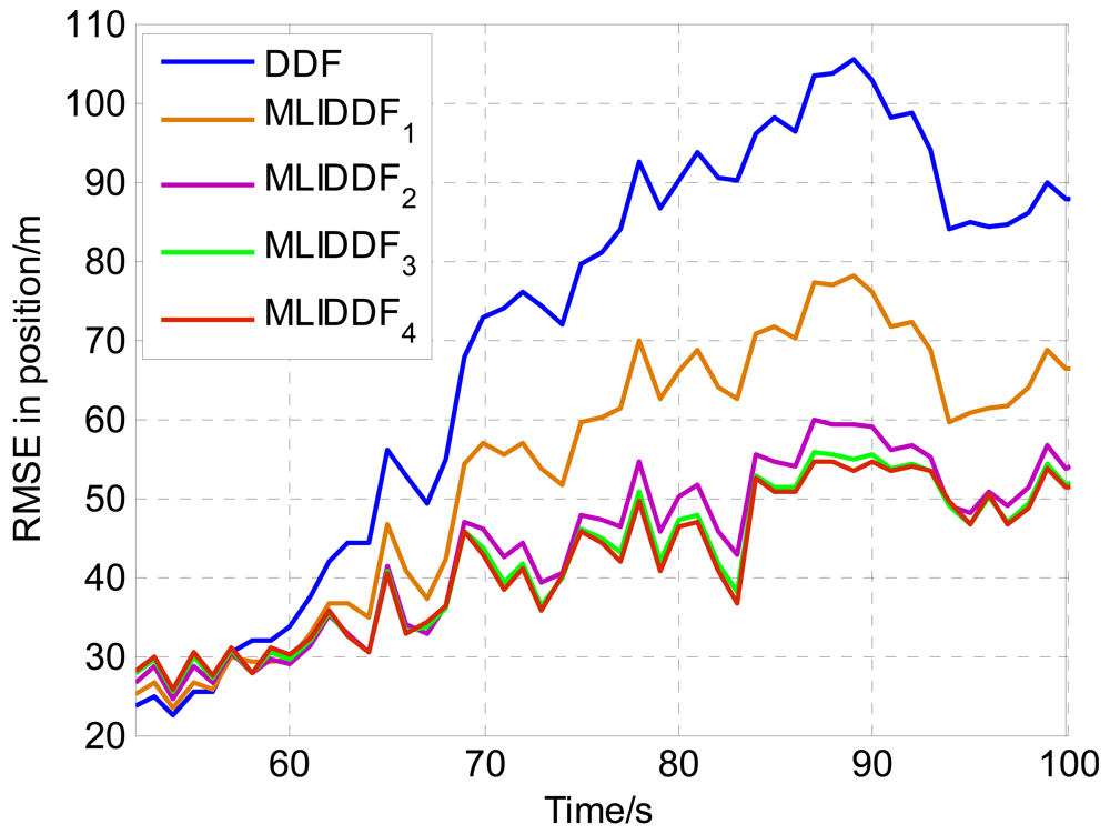
In order to analyze the impact of iteration numbers on performance of the MLIDDF algorithm, the MLIDDFs with various iteration numbers are applied to position estimation of maneuvering target. Figure 4 shows the RMSEs of DDF and MLIDDFs with various numbers in position. From Figure 4, the RMSE in position for the MLIDDF with iteration number 2 begins to decrease largely comparable to that of DDF. The RMSE in position for MLIDDF with iteration number 5 significantly reduce, and the MLIDDF algorithm has very fast convergence rate. The RMSE of the position for MLIDDF decreases slowly when the iteration number is greater than 8; the reason is that the sequence generated has basically reached the maximum likelihood surface when the iteration termination condition is met.
3.2. State Estimation of Reentry Ballistic Target
3.2.1. Simulation Scene
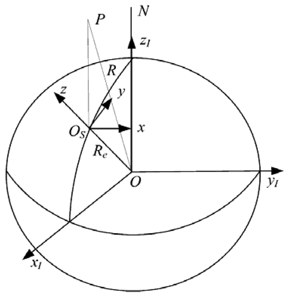
The relative location of the ballistic target re-entry (BTR) and the radar are shown in Figure 5. The inertial coordinate system (ECI-CS) OxIyIzI shown in Figure 5 is a right-handed system with the origin O at the Earth's center, axis OxI pointing in the vernal equinox direction, axis OzI pointing in the direction of the North Pole N. Its fundamental plane OxIyI coincides with the Earth's equatorial plane.
Assume that the radar is situated at the surface of the Earth and considering the orthogonal coordinate reference system named East-North-Up coordinates system (ENU-CS) Osxyz has its origin at the location of the radar. In this system, z is directed along the local vertical and x and y lie in a local horizontal plane, with x pointing east and y pointing north. Assuming that the Earth is spherical and non-rotating and the forces acting on the target are only gravity and drag [20], we can derive the following state equation according to the kinematics of the ballistic re-entry object in the reentry phase in ENU-CS:
Process noise wk is assumed to be white noise with zero mean; its covariance is approximately modeled as [2]:
According to relative geometry, the measurement equation in the ENU-CS is described as:
The measurement noise vk is assumed to be white noise with zero mean and covariance:
3.2.2. Numerical Results and Analysis
The parameters used in simulation were: T = 0.1 s, q1 = 5 m2/s3, q2 = 5 kg2/m4s. The initial position and magnitude of the velocity: x0 = 232 km, y0 = 232 km, z0 = 90 km and v0 = 3,000 m/s, and the initial elevation and azimuth angle: E0 = 7π/6 and A0 = π/4. The ballistic coefficient was selected as β = 4,000 kg/m2. The error standard deviations of the measurements were selected as σR = 100 m, σE = 0.017 rad, and σA = 0.017 rad. A threshold ε = 10 was set in the IUKF and IDDF, and a maximum iteration number Nmax = 8 was predetermined.
From the above parameters given, we can obtain the initial true state:
To compare the performance of the various filter algorithms, we also use RMSE in the position, velocity and ballistic coefficient. The position RMSE at k time of the ballistic target re-entry is defined as:
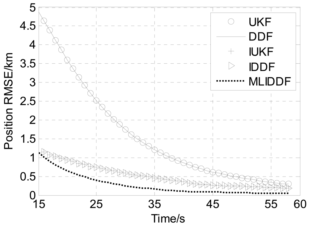
Figures 6–8 shows the position, velocity and ballistic coefficient RMSEs, respectively, for the various filters in an interval of 15–58 s. The initial state estimate x̂0 is chosen randomly from x̂0 ∼
(x0, P0) in each run. All the filters are initialized with the same condition in each run. We make 100 independent Monte Carlo runs.
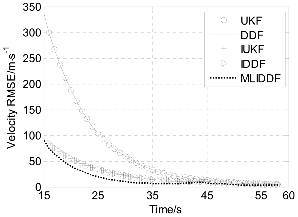
From Figure 6 we can see that the position RMSE of the MLIDDF is much less than the UKF and DDF because of the use of the current measurement in the step of the iteration measurement update of the MLIDDF, and is less than the IUKF and IDDF owing to involving the proposed iteration strategy, so the estimates provided by the MLIDDF are markedly better than those of the UKF and DDF algorithms, and are better than those of IUKF and IDDF algorithms. The MLIDDF also shows a significant improvement over the other filters in the estimation of the velocity, as evidenced by Figure 7.
As to the estimation of the ballistic coefficient, in the Figure 8, we can see that there is no improvement in the RMSE in the initial interval of the observation period (t < 35 s) because there is no effective information about it, while in the remaining period (35 s < t < 58 s) the ballistic coefficient RMSE is decreased because the effective information about the ballistic coefficient from the latest measurement is fully used. Especially, Figure 8 illustrates that toward the end of the trajectory the estimates provided by the MLIDDF are markedly better than those of the UKF, DDF, IUKF and IDDF algorithms.
Meanwhile, we observe from Figures 6–8 that the UKF and DDF have almost the same performance in the problem and the performance of IUKF and IDDF algorithms are almost identical.
For further comparison of performance for the various filters, the average accumulated position mean-square root error (AMSRE) is defined as follows:
From Table 2, it is seen that the position AMSRE for the MLIDDF algorithm is reduced by 62% compared to the UKF and DDF, by 7% compared to IUKF and IDDF. The velocity AMSRE for the MLIDDF algorithm is reduced by 23% compared to the UKF and DDF algorithms. The ballistic coefficient AMSRE for the MLIDDF algorithm is reduced by 7% compared to the UKF and DDF algorithms. Although the ballistic coefficient AMSRE for the MLIDDF algorithm has no significant reduction, we can see that it is reduced significantly compared to the UKF, DDF, IUKF and IDDF algorithms, hence, the MLIDDF is preferred over the other filters in the light of position, velocity and ballistic coefficient AMSREs.
From Table 3, we can see the runtime of MLIDDF is less than that of the IUKF algorithm, and is more than those of UKF, DDF, and IDDF algorithms, so the accuracy of the MLIDDF algorithm is improved at the cost of an increased computational burden. Meanwhile, we can observe the AMSREs for the UKF and DDF in position, velocity and ballistic coefficient are almost identical, and the AMSREs of the IUKF and IDDF are almost the same. Therefore, on the basis of the simulation results presented in Figures 6–8 and Table 2, one can draw the conclusion that the MLIDDF yields a superior performance over the other filters.
4. Conclusions and Future Work
In this study, we provide the maximum likelihood based iterated divided difference filter which inherits the virtues of the divided difference filter and contains the iteration process in the measurement update step. The sequence obtained is guaranteed to move up the likelihood surface using the iteration termination condition based on the maximum likelihood surface. The maximum likelihood based iterated divided difference is implemented easily and is derivative-free. We apply the new filter to state estimation for a ballistic target re-entry scenario and compare its performance against the unscented Kalman filter, divided difference filter, iterated unscented Kalman filter and iterated divided difference filter with the traditional termination criteria. Simulation results demonstrate that the maximum likelihood-based iterated divided difference is much more effective than the other filters. The maximum likelihood-based iterated divided difference greatly improves the performance of state estimation and has a shorter convergence time.
Future work may focus on the applications of the maximum likelihood iteration divided difference filter to remove the outliers which is a serious deviation from the sample and caused by blink and subjective eye movement in video nystagmus signal samples of pilot candidates.
Acknowledgments
This work was partially supported by Grants No. 30871220 from National Natural Science Foundation of China and No. 2007AA010305 from Subprojects of National 863 Key Projects.
References
- Grewal, M.S.; Andrews, A.P. Kalman Filtering: Theory and Practice Using Matlab, 3rd ed.; John Wiley & Sons, Inc: Hoboken, NJ, USA, 2008; pp. 169–201. [Google Scholar]
- Bar-Shalom, Y.; Li, X.R.; Kirubarajan, T. Estimation with Applications to Tracking and Navigation; John Wiley &Son, Inc: Hoboken, NJ, USA, 2001; pp. 371–420. [Google Scholar]
- Jazwinski, A.H. Stochastic Process and Filtering Theory; Academic Press: Waltham, MA, USA, 1970; pp. 332–365. [Google Scholar]
- Julier, S.J.; Uhlmann, J.K. Unscented filtering and nonlinear estimation. Proc. IEEE 2004, 92, 401–422. [Google Scholar]
- Athans, M.; Wishner, R.P.; Bertolini, A. Suboptimal state estimation for continuous-time nonlinear system from discrete noisy measurements. IEEE Trans. Autom. Control 1968, 13, 504–514. [Google Scholar]
- Gelb, A. Applied Optimal Estimation; The MIT Press: Cambridge, MA, USA, 1974; pp. 180–228. [Google Scholar]
- Lefebvre, T.; Bruyninckx, H.; de Schutter, J. Kalman filters for non-linear systems: A comparison of performance. Int. J. Control 2004, 77, 639–653. [Google Scholar]
- Bell, B.M.; Cathey, F.W. The iterated Kalman filter update as a Gauss-Newton method. IEEE Trans. Autom. Control 1993, 38, 294–297. [Google Scholar]
- Johnston, L.A.; Krishnamurthy, V. Derivation of a sawtooth iterated extended Kalman smoother via the AECM algorithm. IEEE Trans. Signal Proc. 2001, 49, 1899–1909. [Google Scholar]
- Zhan, R.; Wan, J. Iterated unscented Kalman filter for passive target tracking. IEEE Trans. Aerosp. Electron. Syst. 2007, 43, 1155–1163. [Google Scholar]
- Schei, T.S. A finite-difference method for linearization in nonlinear estimation algorithms. Modeling Identif. Control 1998, 19, 141–152. [Google Scholar]
- Julier, S.; Uhlmann, J.; Durrant-Whyte, H.F. A new method for the nonlinear transformation of means and covariances in filters and estimations. IEEE Trans. Autom. Control 2000, 45, 477–482. [Google Scholar]
- Julier, S.J.; Uhlmann, J.K.; Durrant-Whyte, H.F. A New Approach for Filtering Nonlinear Systems. Proceedings of the American Control Conference, Seattle, WA, USA; 1995; pp. 1628–1632. [Google Scholar]
- Nørgaard, M.; Poulsen, N.K.; Ravn, O. New developments in state estimation for nonlinear systems. Automatica 2000, 36, 1627–1638. [Google Scholar]
- Nørgaard, M.; Poulsen, N.K.; Ravn, O. Advances in Derivative-Free State Estimation for Nonlinear Systems; Technical Report; Technical University of Denmark: Lyngby, Denmark, 2000. [Google Scholar]
- van der Merwe, R.; Wan, E. Sigma-Point Kalman Filters for Probabilistic Inference in Dynamic State-Space Models. 2004. Available online: http://en.scientificcommons.org/42640909 (accessed on 26 June 2012). [Google Scholar]
- Gordon, N.; Salmond, D.J.; Smith, A.F.M. Novel approach to nonlinear non-Gaussian Bayesian state estimation. IEEE Proc. 1993, 140, 107–113. [Google Scholar]
- Arulampalam, M.S.; Maskell, S.; Gordon, N.; Clapp, T. A tutorial on particle filters for online nonlinear/non-Gaussian Bayesian tracking. IEEE Trans. Signal Proc. 2002, 50, 174–188. [Google Scholar]
- Arasaratnam, I.; Haykin, S. Cubature Kalman filters. IEEE Trans. Autom. Control 2009, 54, 1254–1269. [Google Scholar]
- Li, X.R.; Jilkov, V.P. A survey of maneuvering target tracking-part II: Ballistic target models. Proc. SPIE 2001, 4473, 559–581. [Google Scholar]
- Farina, A.; Ristic, B.; Benvenuti, D. Tracking a ballistic target: Comparison of several nonlinear filters. IEEE Trans. Aerosp. Electron. Syst. 2002, 38, 854–867. [Google Scholar]


| Various filters | Advantage | Disadvantage |
|---|---|---|
| EKF | Less runtime | Calculation of Jacobian |
| Second-order EKF | high accuracy | Calculation of Jacobian and Hessian |
| IEKF | high accuracy | Calculation of Jacobian |
| UKF | Derivative-free | more runtime |
| IUKF-VS | Derivative-free, high accuracy | more runtime |
| FDF | Derivative-free, Less runtime | Lower accuracy |
| DDF | Derivative-free | Low accuracy |
| PF | Derivative-free | Heavy computational burden |
| Various algorithms | AMSREp(m) | AMSREv(m/s) | AMSREβ(kg/m2) |
|---|---|---|---|
| UKF | 2521.684 | 329.911 | 155.735 |
| DDF | 2521.573 | 329.903 | 155.276 |
| IUKF | 1035.340 | 259.173 | 149.603 |
| IDDF | 1035.273 | 260.771 | 149.756 |
| MLIDDF | 968.746 | 255.916 | 144.953 |
| Various algorithms | Runtime(s) |
|---|---|
| UKF | 1.0840 |
| DDF | 0.2888 |
| IUKF | 1.9918 |
| IDDF | 0.5133 |
| MLIDDF | 1.3074 |
© 2012 by the authors; licensee MDPI, Basel, Switzerland. This article is an open access article distributed under the terms and conditions of the Creative Commons Attribution license (http://creativecommons.org/licenses/by/3.0/).
Share and Cite
Wang, C.; Zhang, J.; Mu, J. Maximum Likelihood-Based Iterated Divided Difference Filter for Nonlinear Systems from Discrete Noisy Measurements. Sensors 2012, 12, 8912-8929. https://doi.org/10.3390/s120708912
Wang C, Zhang J, Mu J. Maximum Likelihood-Based Iterated Divided Difference Filter for Nonlinear Systems from Discrete Noisy Measurements. Sensors. 2012; 12(7):8912-8929. https://doi.org/10.3390/s120708912
Chicago/Turabian StyleWang, Changyuan, Jing Zhang, and Jing Mu. 2012. "Maximum Likelihood-Based Iterated Divided Difference Filter for Nonlinear Systems from Discrete Noisy Measurements" Sensors 12, no. 7: 8912-8929. https://doi.org/10.3390/s120708912