Evaluation of a 433 MHz Band Body Sensor Network for Biomedical Applications

 ,
,
Abstract
:
1. Introduction
2. Methods and Material
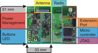
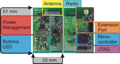
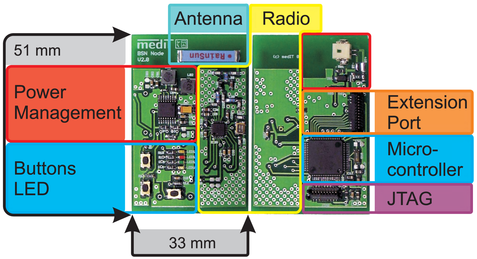
2.1. System Architecture
- Microcontroller (MSP430F1611, Texas Instruments Inc., Dallas, TX, USA)
- Power management (TPS61131, Texas Instruments Inc., Dallas, TX, USA)
- Wireless Transceiver (CC1101, Texas Instruments Inc., Dallas, TX, USA)
- Extension port (Microstac12, Erni Electronics GmbH, Adelberg, Germany)
2.2. Improvements in IPANEMA Generation 2.5
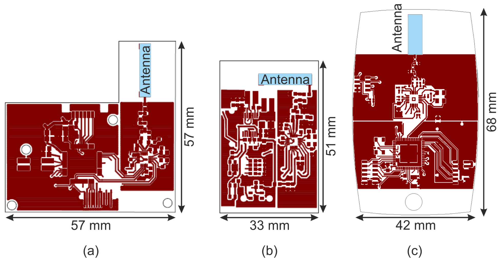
2.2.1. Hardware
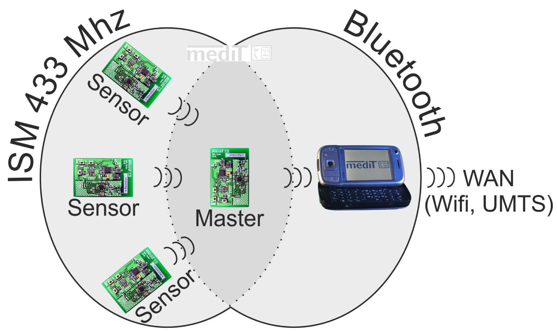
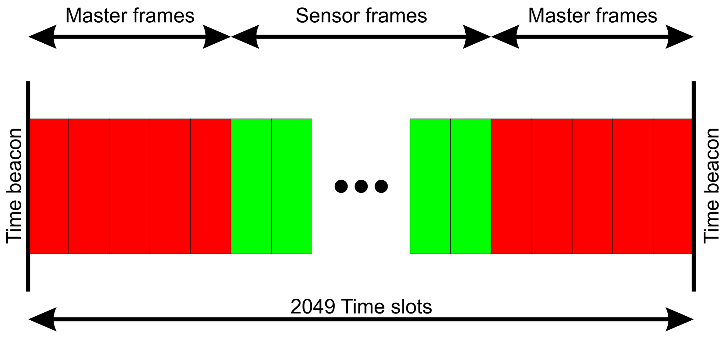
2.2.2. Network
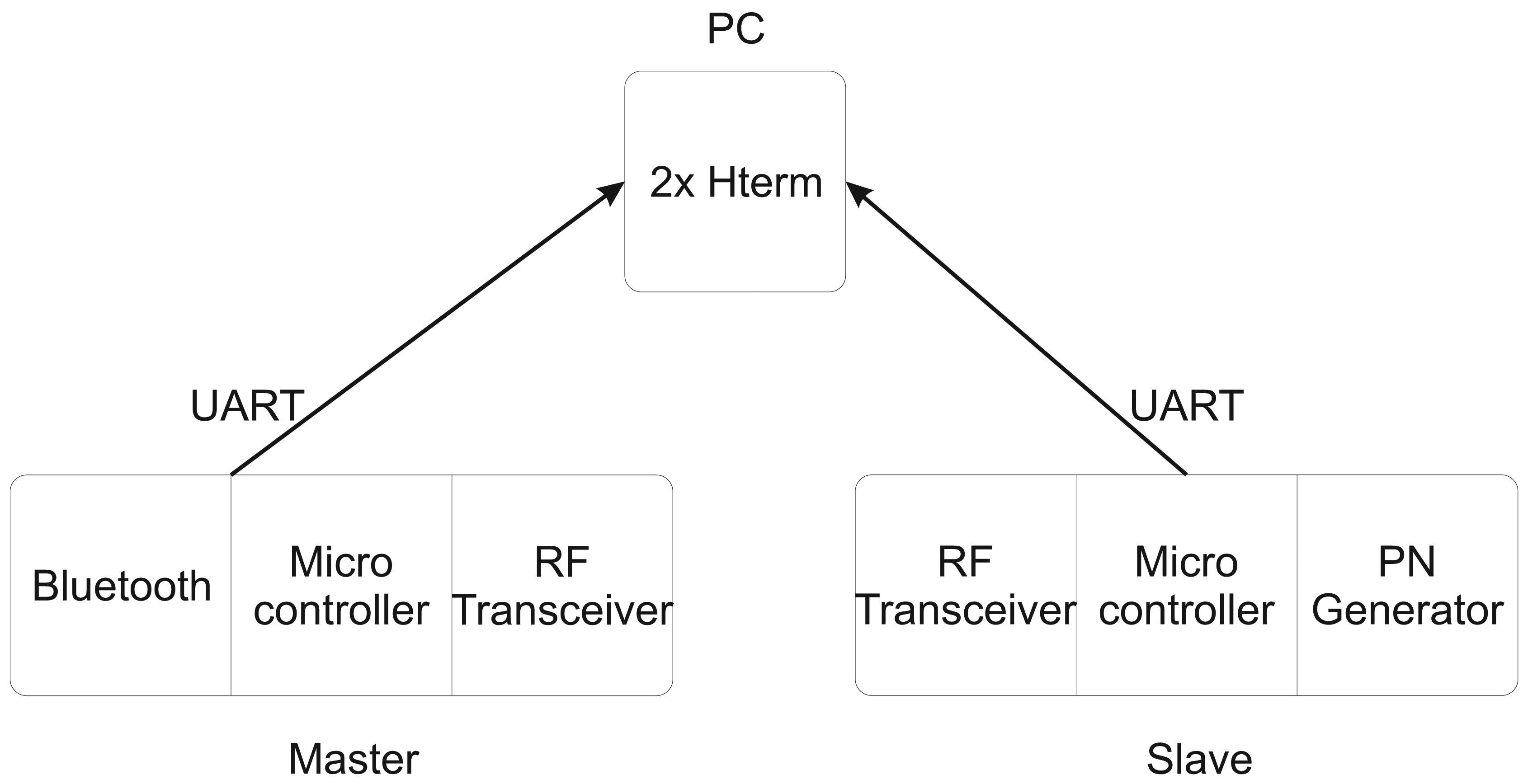
2.3. Validation of Wireless Communication Interface
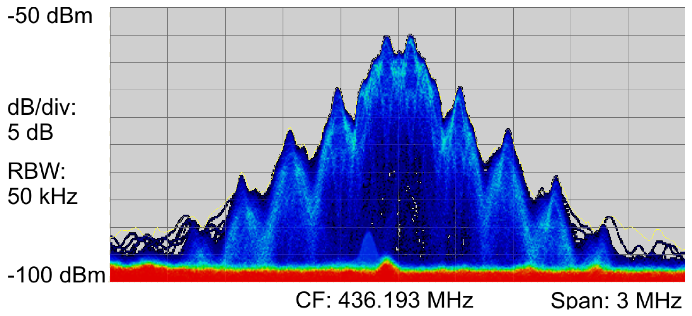
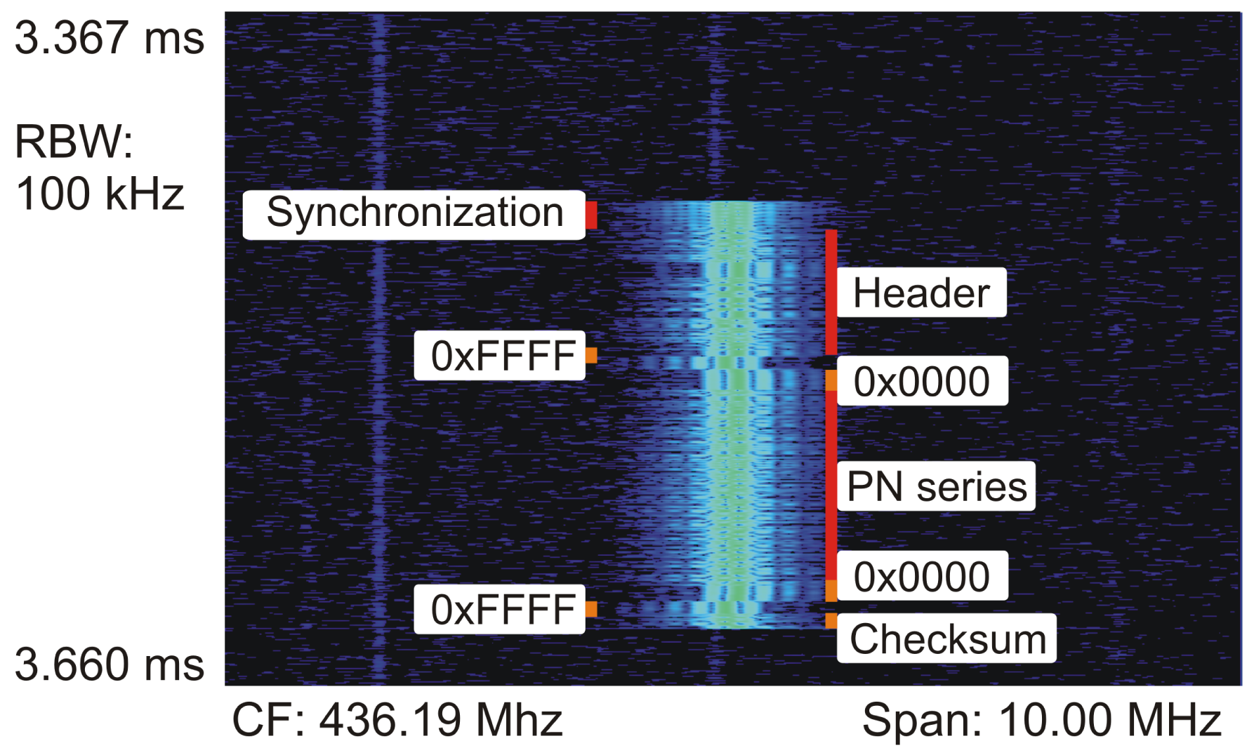
2.3.1. Spectrum Analysis
| P | Measured transmission power |
| P0 | Reference power of 1 mW |
| LSignal | Signal power |
| N0 | Noise power |
2.3.2. PLR Measurements
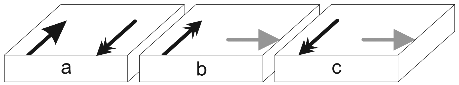
- Single/dual slave node lab setup with variation of distance and orientation
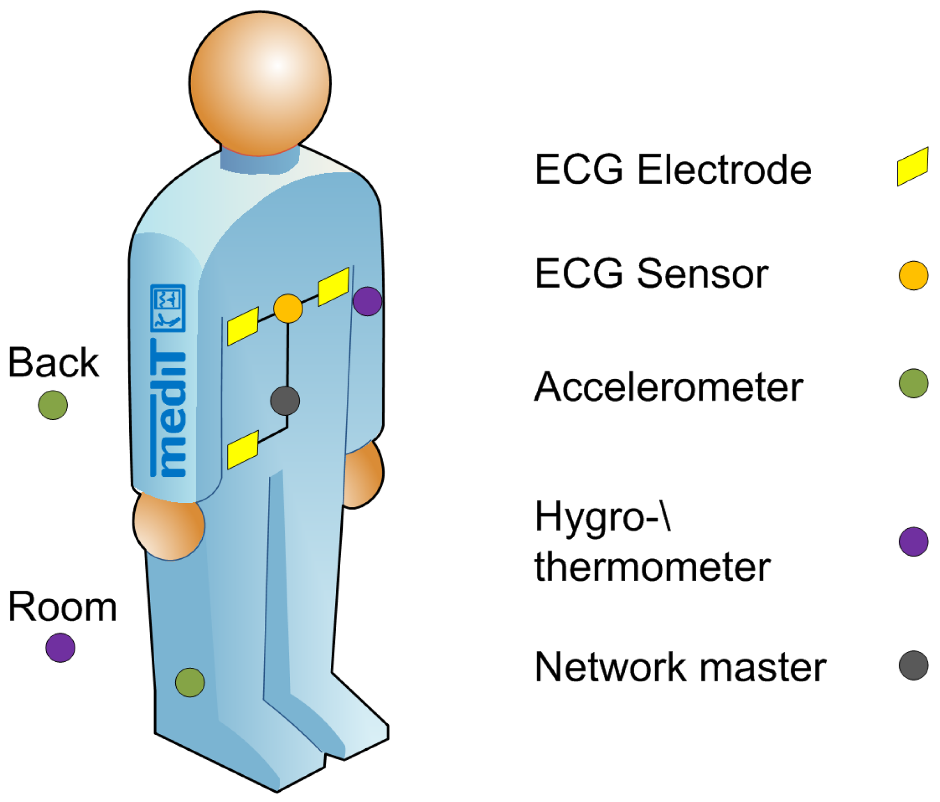
- Five slave nodes on-body measurement
- Identification of packet loss: Have all packets been received by the master node?
- Identification of bit errors: Is the received PN series identical to the transmitted series?
- Error type
- Packet size
- Position of the bit error in the payload
- Original PN series
Lab setup Measurements
On-Body Measurements
- Indoor treadmill
- Outdoor running track
- Climate chamber
3. Results and Discussion
3.1. Spectrum Analysis
3.2. PLR Measurements
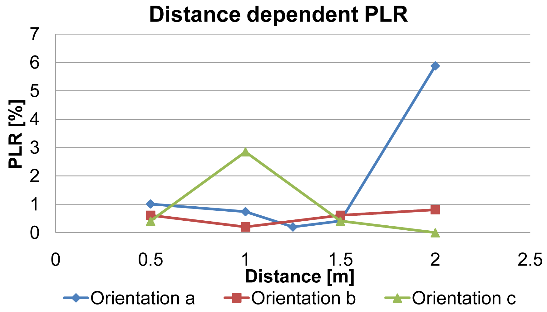
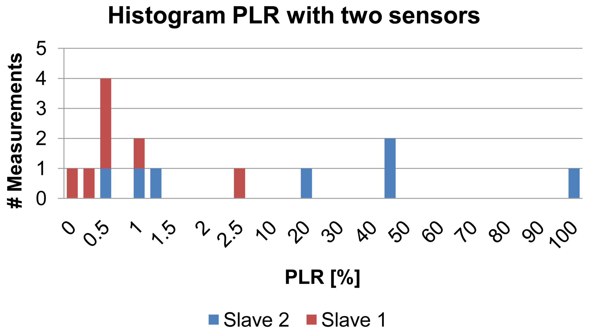
3.2.1. Lab Setup Measurements
3.2.2. On-body Measurements
3.3. Comparison with ZigBee-based Systems
4. Conclusions
Acknowledgments
References
- Yang, G.Z.; Yacoub, M. Body Sensor Networks, 1st ed.; Springer-Verlag Inc.: New York, NY, USA, 2006. [Google Scholar]
- Hao, Y.; Foster, R. Wireless body sensor networks for health-monitoring applications. Physiol. Meas. 2008, 29, R27. [Google Scholar]
- Patel, M.; Wang, J. Applications, challenges, and prospective in emerging body area networking technologies. IEEE Wirel. Commun. 2010, 17, 80–88. [Google Scholar]
- Hundley, R.O.; Gritton, E.C. Future technology-driven revolutions in military operations. Doc. Brief. Series 1994, 110, 1–105. [Google Scholar]
- Jovanov, E.; O'Donnell Lords, A.; Raskovic, D.; Cox, P.G.; Adhami, R.; Andrasik, F. Stress monitoring using a distributed wireless intelligent sensor system. IEEE Eng. Med. Biol. Mag. 2003, 22, 49–55. [Google Scholar]
- Pantelopoulos, A.; Bourbakis, N.G. A Survey on Wearable Sensor-Based Systems for Health Monitoring and Prognosis. IEEE Trans. Syst. Man Cybern.—Part C: Appl. Rev. 2010, 40, 1–12. [Google Scholar]
- Ullah, S.; Khan, P.; Ullah, N.; Saleem, S.; Higgins, H.; Kwak, K. A review of wireless body area networks for medical applications. Int. J. Commun. Netw. Syst. Sci. 2009. [Google Scholar] [CrossRef]
- Kohler, F.; Schieber, M.; Lucke, S.; Heinze, P.; Henke, S.; Matthesius, G.; Pferdt, T.; Wegertseder, D.; Stoll, M.; Anker, S.D. “Partnership for the Heart”—Development and testing of a new remote patient monitoring system. Dtsch. Med. Wochenschr. 2007, 132, 458–460. [Google Scholar]
- Palmer, M.; Steffen, C.; Iakovidis, I.; Giorgio, F. European commission perspective: Telemedicine for the benefit of patients. Chronic Dis. Manag. Remote Patient Monit. 2009, 15, 13–15. [Google Scholar]
- Penders, J.; Gyselinckx, B.; Vullers, R.; de Nil, M.; Nimmala, V.S.R.; van de Molengraft, J.; Yazicioglu, F.; Torfs, T.; Leonov, V.; Merken, P.; et al. Human++: From Technology to Emerging Health Monitoring Concepts. Proceedings of the 5th International Summer School and Symposium on Medical Devices and Biosensors (ISSS-MDBS), Hong Kong, China, 1–3 June 2008; pp. 94–98.
- Jovanov, E.; Poon, C.; Yang, G.Z.; Zhang, Y.T. Guest editorial body sensor networks: From theory to emerging applications. IEEE Trans. Inf. Technol. Biomed. 2009, 13, 859–863. [Google Scholar]
- Lai, D.; Begg, R.; Palaniswami, M. Healthcare Sensor Networks: Challenges Toward Practical Implementation; CRC Press: Boca Raton, FL, USA, 2011. [Google Scholar]
- Kjeldskov, J.; Skov, M. Exploring context-awareness for ubiquitous computing in the healthcare domain. Pers. Ubiquitous Comput. 2007, 11, 549–562. [Google Scholar]
- Colas, J.; Guillen, A. The Biomedical Engineer as a Driver for Health Technology Innovation. Proceedings of the IEEE EMBS 32nd Annual International Conference, Buenos Aires, Argentina, 31 August–4 September 2010.
- Ballerstadt, R.; Kholodnykh, A.; Evans, C.; Boretsky, A.; Motamedi, M.; Gowda, A.; McNichols, R. Affinity-based turbidity sensor for glucose monitoring by optical coherence tomography: Toward the development of an implantable sensor. Anal. Chem. 2007, 79, 6965–6974. [Google Scholar]
- Gomez, E.J.; Perez, M.E.H.; Vering, T.; Rigla Cros, M.; Bott, O.; Garcia-Saez, G.; Pretschner, P.; Brugues, E.; Schnell, O.; Patte, C.; et al. The INCA system: A further step towards a telemedical artificial pancreas. IEEE Trans. Inf. Technol. Biomed. 2008, 12, 470–479. [Google Scholar]
- Ying, H.; Schloesser, M.; Schnitzer, A.; Schafer, T.; Schlaefke, M.; Leonhardt, S.; Schiek, M. Distributed intelligent sensor network for rehabilitation of parkinson's patients. IEEE Trans. Inf. Technol. Biomed. 2010, 15, 268–276. [Google Scholar]
- Lo, B.; Yang, G.Z. Key Technical Challenges and Current Implementations of Body Sensor Networks. Proceedings of the 2nd International Workshop on Body Sensor Networks, London, UK, 12–13 April 2005.
- Alomainy, A.; Hao, Y.; Hu, X.; Parini, C.G.; Hall, P.S. UWB on-body radio propagation and system modelling for wireless body-centric networks. IEE Proc. Commun. 2006, 153, 107–114. [Google Scholar]
- Pei, J.S.; Kapoor, C.; Graves-Abe, T.L.; Sugeng, Y.P.; Ferzli, N.; Lynch, J.P. Investigation of data quality in a wireless sensing unit composed of off-the-shelf components. Proc. SPIE 2008, 5768, 118–128. [Google Scholar]
- Takizawa, K.; Watanabe, K.; Kumazawa, M.; Hamada, Y.; Ikegami, T.; Hamaguchi, K. Performance Evaluation of Wearable Wireless Body Area Networks during Walking Motions in 444.5 MHz and 2450 MHz. Proceedings of the IEEE EMBS 32nd Annual International Conference, Buenos Aires, Argentina, 31 August–4 September 2010.
- Alomainy, A.; Yang, H.; Pasveer, F. Numerical and experimental evaluation of a compact sensor antenna for healthcare devices. IEEE Trans. Biomed. Circuits Syst. 2007, 1, 242–249. [Google Scholar]
- Cavalcanti, D.; Schmitt, R.; Soomro, A. Performance Analysis of 802.15.4 and 802.11e for Body Sensor Network Applications. Proceedings of the 4th International Workshop on Wearable and Implantable Body Sensor Networks (BSN); Springer: Aachen, Germany, 2007. Volume 13. p. 9. [Google Scholar]
- Sikora, A.; Groza, V.F. Coexistence of IEEE 802.15.4 with Other Systems in the 2.4 GHz-ISM-Band. Proceedings of the IEEE Instrumentation and Measurement Technology Conference (IMTC), Ottawa, ON, Canada, 16–19 May 2005; Volume 3. pp. 1786–1791.
- Yun, D.; Kang, J.; Kim, J.E.; Kim, D. A Body Sensor Network Platform with Two-Level Communications. Proceedings of the IEEE International Symposium on Consumer Electronics (ISCE), Piscataway, NJ, USA, 20–23 June 2007; pp. 1–6.
- Beute, J. Fast-prototyping Using the BTnode Platform. Proceedings of the Proceedings Design, Automation and Test in Europe (DATE), Munich, Germany, 6–10 March 2006; Volume 1. pp. 1–6.
- Paradiso, J.; Borriello, G.; Bonato, P. Implantable electronics. Pervasive Comput. IEEE 2008, 7, 12–13. [Google Scholar]
- Weinstock, R.S. Closing the loop: Another step forward. Diabetes Care 2011, 34, 2136–2137. [Google Scholar]
- Jetzki, S.; Kiefer, M.; Walter, M.; Leonhardt, S. Concepts for a Mechatronic Device to Control Intracranial Pressure. Proceedings of the 4th IFAC Symposium on Mechatronic Systems, Heidelberg, Germany, 12–14 September 2006; Volume 4. pp. 25–29.
- Panescu, D. Emerging Technologies [wireless communication systems for implantable medical devices]. IEEE Eng. Med. Biol. Mag. 2008, 27, 96–101. [Google Scholar]
- Kim, S.; Beckmann, L.; Pistor, M.; Cousin, L.; Walter, M.; Leonhardt, S. A Versatile Body Sensor Network for Health Care Applications. Proceedings of the 5th International Conference on Intelligent Sensors, Sensor Networks and Information Processing (ISSNIP), Melbourne, Australia, 7–9 December 2009; pp. 175–180.
- Kim, S.; Pistor, M.; Walter, M.; Leonhardt, S. Development of a Body Sensor Network in the 433 MHz Base Band for Medical Signal Acquisition. Proceedings of the 13th International Student Conference on Electrical Engineering POSTER, Prague, Czech Republic, 21 May 2009.
- CrossbowTechnology. Mica2 Datasheet, 2004. Avaiable online: http://bullseye.xbow.com:81/Products/productdetails.aspx?sid=174 (accessed on 10 October 2012).
- Volmer, A.; Orglmeister, R. Wireless Body Sensor Network for Low-Power Motion-Tolerant Syncronized Vital Sign Measurment. Proceedings of the Engineering in Medicine and Biology Society, 2008. EMBS 2008. 30th Annual International Conference of the IEEE, Vancouver, BC, Canada, 20–24 August 2008; pp. 3422–3425.
- Simon, D. An Embedded Software Primer; Addison-Wesley Professional: Toronto, Canada, 1999. [Google Scholar]
- Xu, L.S.; Meng, M.Q.H.; Chao, H. Effects of dielectric values of human body on specific absorption rate following 430, 800, and 1200 MHz RF exposure to ingestible wireless device. IEEE Trans. Inf. Technol. Biomed. 2010, 14, 52–59. [Google Scholar]
- Petrie, C.S.; Connelly, J.A. A Noise-Based Random Bit Generator IC For Applications in Cryptography. Proceedings of the 1998 IEEE International Symposium on Circuits and Systems, 1998, Atlanta, GA, USA, 31 May–3 June 1998; pp. 197–200.
- Shin, S.Y.; Park, H.S.; Choi, S.; Kown, W.H. Packet error rate analysis of ZigBee under WLAN and bluetooth interferences. IEEE Trans. Wirel. Commun. 2007, 6, 2825–2830. [Google Scholar]
- Incel, O.; Mullender, S.; Jansen, P.; Dulman, S. Measurements on the Efficiency of Overlapping Channels. Proceedings of 2007 2nd IEEE Workshop on the Networking Technologies for Software Define Radio Networks, San Diego, CA, USA, 18–21 June 2007; pp. 59–60.
- Kammeyer, K.D. Nachrichtenübertragung, 3rd ed.; B.G. Teubner GmbH: Leipzig, Germany, 2004. [Google Scholar]
- Tektronix. Fundamentals of Real-Time Spectrum Analysis; Tektronix: Beaverton, OR, USA, 2009. [Google Scholar]
- Rahman, M.; Hong, C.; Lee, S.; Bang, Y.C. Atlas: A traffic load aware sensor Mac design for collaborative body area sensor networks. Sensors 2011, 11, 11560–11580. [Google Scholar]
- Xia, F.; Tian, Y.C.; Li, Y.; Sung, Y. Wireless sensor/actuator network design for mobile control applications. Sensors 2007, 7, 2157–2173. [Google Scholar]
- Petrova, M.; Riihijarvi, J.; Mahonen, P.; Labella, S. Performance Study of IEEE 802.15.4 Using Measurements and Simulations. Proceedings of the Wireless Communications and Networking Conference, 2006. WCNC 2006. IEEE, Las Vegas, NV, USA, 3–6 April 2006; Volume 1. pp. 487–492.
- Shopov, M.; Petrova, G.; Spasov, G. Evaluation of Zigbee-based body sensor networks. Ann. J. Electron. 2011, 5, 60–63. [Google Scholar]
- Llosa, J.; Vilajosana, I.; Vilajosana, X.; Navarro, N.; Suriñach, E.; Marquès, J. REMOTE, a wireless sensor network based system to monitor rowing performance. Sensors 2009, 9, 7069–7082. [Google Scholar]
- Dhamdhere, A.D. Experiments with wireless sensor networks for real-time athlete monitoring. Proceedings of 2010 IEEE 35th Conference on Local Computer Networks (LCN), Denver, CO, USA, 11–14 October 2010; pp. 938–945.
- Armstrong, S. Wireless connectivity for health and sports monitoring: A review. Br. J. Sports Med. 2007, 41, 285–289. [Google Scholar]


| Orientation | Avg. Packets Send | Avg. TX Rate [B/s] | n |
|---|---|---|---|
| a | 502.6 | 47.81 | 2513 |
| b | 493.25 | 47.87 | 1973 |
| Sensor | Location | Sampl. Freq. [Hz] | Packet Length [bytes] |
|---|---|---|---|
| ECG | Chest | 512 | 54 |
| Accelerometer | Left ankle lateral | 50 | 42 |
| Accelerometer | Back above coccyx | 50 | 42 |
| Hygro-/thermometer | Left upper arm lateral | 0.5 | 46 |
| Hygro-/thermometer | Room | 0.5 | 46 |
| Parameter | Mean Value | ± Standard Deviation |
|---|---|---|
| Age (a) | 29 | ± 4 |
| Height (cm) | 181 | ± 5 |
| Weight (kg) | 73 | ± 7 |
| Antenna Orientation | μ PLR [%] | σ PLR [%] | n |
|---|---|---|---|
| a | 1.65 | 2.39 | 2513 |
| b | 0.56 | 0.26 | 1973 |
| c | 0.92 | 1.30 | 1969 |
| Sensor Number | μ PLR [%] | σ PLR [%] | n |
|---|---|---|---|
| 1 | 0.75 | 0.83 | 3454 |
| 2 | 30.39 | 36.48 | 3454 |
| Sensor | Indoor PLR [%] | Outdoor PLR [%] | Climate PLR [%] | |
|---|---|---|---|---|
| ECG | Mean | 2.10 | 3.61 | 0.52 |
| Std. | 7.48 | 7.25 | 1.66 | |
| n | 2,155,776 | 396,735 | 1,677,680 | |
| ACC1FOOT | Mean | 3.61 | 4.18 | 2.75 |
| Std. | 6.63 | 6.06 | 3.98 | |
| n | 471,164 | 82,589 | 346,555 | |
| ACC2BACK | Mean | 2.04 | 2.07 | 1.10 |
| Std. | 5.49 | 4.42 | 1.65 | |
| n | 469,639 | 67,776 | 345,739 | |
| HYGRO1SKIN | Mean | 2.71 | 3.71 | 1.68 |
| Std. | 5.84 | 8.67 | 1.90 | |
| n | 19,207 | 1366 | 15,617 | |
| HYGRO2ROOM | Mean | 2.11 | - | 1.45 |
| Std. | 4.92 | - | 1.71 | |
| n | 21,977 | - | 16,099 |
© 2013 by the authors; licensee MDPI, Basel, Switzerland. This article is an open access article distributed under the terms and conditions of the Creative Commons Attribution license (http://creativecommons.org/licenses/by/3.0/).
Share and Cite
Kim, S.; Brendle, C.; Lee, H.-Y.; Walter, M.; Gloeggler, S.; Krueger, S.; Leonhardt, S. Evaluation of a 433 MHz Band Body Sensor Network for Biomedical Applications. Sensors 2013, 13, 898-917. https://doi.org/10.3390/s130100898
Kim S, Brendle C, Lee H-Y, Walter M, Gloeggler S, Krueger S, Leonhardt S. Evaluation of a 433 MHz Band Body Sensor Network for Biomedical Applications. Sensors. 2013; 13(1):898-917. https://doi.org/10.3390/s130100898
Chicago/Turabian StyleKim, Saim, Christian Brendle, Hyun-Young Lee, Marian Walter, Sigrid Gloeggler, Stefan Krueger, and Steffen Leonhardt. 2013. "Evaluation of a 433 MHz Band Body Sensor Network for Biomedical Applications" Sensors 13, no. 1: 898-917. https://doi.org/10.3390/s130100898