A Near-Optimal Distributed QoS Constrained Routing Algorithm for Multichannel Wireless Sensor Networks

Abstract

One of the important applications in Wireless Sensor Networks (WSNs) is video surveillance that includes the tasks of video data processing and transmission. Processing and transmission of image and video data in WSNs has attracted a lot of attention in recent years. This is known as Wireless Visual Sensor Networks (WVSNs). WVSNs are distributed intelligent systems for collecting image or video data with unique performance, complexity, and quality of service challenges. WVSNs consist of a large number of battery-powered and resource constrained camera nodes. End-to-end delay is a very important Quality of Service (QoS) metric for video surveillance application in WVSNs. How to meet the stringent delay QoS in resource constrained WVSNs is a challenging issue that requires novel distributed and collaborative routing strategies. This paper proposes a Near-Optimal Distributed QoS Constrained (NODQC) routing algorithm to achieve an end-to-end route with lower delay and higher throughput. A Lagrangian Relaxation (LR)-based routing metric that considers the “system perspective” and “user perspective” is proposed to determine the near-optimal routing paths that satisfy end-to-end delay constraints with high system throughput. The empirical results show that the NODQC routing algorithm outperforms others in terms of higher system throughput with lower average end-to-end delay and delay jitter. In this paper, for the first time, the algorithm shows how to meet the delay QoS and at the same time how to achieve higher system throughput in stringently resource constrained WVSNs.

1. Introduction

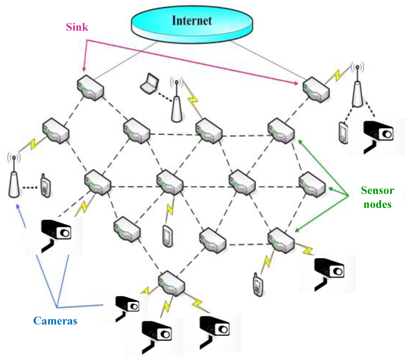
In recent years, Wireless Visual Sensor Networks (WVSNs) have emerged as an interesting field. Popular applications are environmental monitoring, seismic detection, military surveillance, medical monitoring, video surveillance, or the Internet of Things (IoT), etc. [1]. IoT integrates a part of the Future Internet and extends network capabilities to Machine-to-Machine (M2M) communications by a dynamic network infrastructure with self-organization techniques. As compared to a WSN, the camera equipped sensor nodes in WVSNs can capture, process and transmit the real time visual data (images, video). Since the visual data is much larger and complicated than scalar data, delay Quality of Service (QoS) is a challenging issue resource for constrained WVSNs. WVSNs attract more attention on how the camera sensor nodes can cooperatively pass their data more efficiently with minimum delay through the network on a large scale or under realistic physical environmental conditions [2,3]. The architecture of WVSNs is shown in Figure 1.

In WVSNs for video surveillance, the delay is a very important QoS metric, and the delay is highly dependent on the routing strategies. However, delay routing in WVSN is more difficult than in WSN due to the fact visual data is much larger and complicated than scalar data. Furthermore, battery-limited powered and resource (channel-, CPU-) constrained camera nodes make this delay routing problem more challenging in WVSNs. [4]. Basically, for real-time video surveillance applications, meeting the end-to-end delay QoS is the most important criteria. However, due to the limited resources of WVSNs, delay QoS routing decisions should also consider overall resource utilization so that the future video surveillance applications could be also satisfied. Hence, besides meeting the end-to-end delay QoS for each user, minimizing the average delay in WVSNs is also another crucial performance metric. In this paper, for the first time, we consider the delay QoS routing strategy in WVSNs to meet the end-to-end delay QoS for each application and at the same time minimize the average delay.

2. Literature Survey

Delay QoS routing is a challenging issue in WVSNs. Traditional approaches for wireless sensor networks are not efficient or even feasible in a WVSN due to three reasons: first of all, visual data are much bigger and complicated than scalar data, and processing and transmitting visual data will consume much more system resources than scalar data. Secondly, WVSNs need efficient collaborative image processing and coding techniques that can exploit correlation in data collected by adjacent camera sensor nodes. Video coding/compression that has low complexity, produces a low output bandwidth, tolerates losses, and consumes as little power as possible is required. Third, it needs to reliably send the relevant visual data from the camera sensor nodes to aggregation nodes or the sink node in an energy-efficient way [1,2]. This issue is related to the transmission technique that consists of the routing assignment to provide energy efficient and stable routes that meet the end-to-end QoS guarantees [2–4].

In wireless visual sensor networks for real time video surveillance, sensor nodes need to capture and forward the packets to the sinks within an acceptable delay under the limited resource constraints, including embedded vision processing, data communication, and battery energy issues. It is a challenging issue since it needs to meet the end-to-end delay for each application and at the same time optimize the system resource utilization by minimizing the average system delay so that more real-time applications can be granted access in the near future. Existing research on wireless sensor networks address the link scheduling techniques [5], channel assignments [6–8], routing algorithms [9,10], or resource allocations [11–13]. Some of the well-known routing protocols, such as Ad hoc On-demand Distance Vector (AODV), Dynamic Source Routing (DSR), Optimized Link State Routing (OLSR), and Destination Sequenced Distance Vector (DSDV) are the protocols applied to Ad hoc networks, such as MANETs, WMNs, VANETS, etc., that consist of hosts interconnected by routers without a fixed infrastructure that can be arranged dynamically [14]. Even though like in the MANETs, there is no centralized AP or base station in WVSN, sensor nodes are also the relay nodes to forward the data to the sink node. However, without addressing the delay QoS, these approaches are not applicable to real-time applications. In the following, we survey existing approaches on shortest path routing, QoS routing, and routing algorithms. To the best of our knowledge, there is no research addressing the end-to-end delay from the user perspective and at the same time optimizing the system resource utilization by minimizing the average system delay.

2.1. Shortest Path Routing

The routing algorithm is determined by the shortest path and the routing decision for the O-D pair. When a new route is established and all traffic still follows the pre-existing path, this phenomenon is called “session routing” because a path remains in force for the entire user session. The routing metric (i.e., cost) is used to define the path length and can be measured in terms of hops, the mean delay, and even the extent of flow deviation. The mean delay can be used to find the fastest path for routing, and flow deviation can be applied to system optimization routing where each route has equal flow deviation.

2.2. QoS Routing

Quality-of-Service (QoS) is a major issue that can be divided into several factors including the reliability, mean delay, delay jitter, and bandwidth of packet transmissions [15]. Controlling QoS is a challenge faced by the routing of multihop wireless sensor networks with interference [16]. In multichannel wireless sensor networks, transmitted packets may collide in an interference environment if the nodes and neighbors within transmission range use the same channel. This adversely affects system performance and the QoS. Different types of applications have different QoS standards. As such, the QoS routing problems differ by the QoS types requirements of end users and therefore require careful control of channel assignment within an interference environment. By using different and non-overlapping channels, each node can freely communicate with its neighboring nodes (i.e., the nodes within transmission range) without interference. As noted in [15], using multiple channels instead of a single channel in multihop wireless sensor networks has been shown to not only reduce packet contention probability in non-overlapping channels, but to also dramatically improve the network throughput. A channel assignment strategy is necessary to efficiently use multiple channels with commodity hardware; besides, the channel assignment can be changed with significant changes in traffic load or network topology [7,8].

2.3. Routing Protocols

Routing protocols are categorized into table driven and on-demand, based on route calculation. Researches indicate that a Mobile Ad hoc NETwork (MANET) has several characteristics: (1) dynamic topologies; (2) bandwidth-constrained links; (3) energy constrained operation; and (4) limited physical security. Therefore the routing protocols for wired networks cannot be directly used for wireless networks [14,17,18]. The characteristics (1), (2) and (3) are similar to WVSNs, which is the driving force to design a protocol to apply to this case.

Proactive (table-driven) protocols are based on periodic exchange of control messages and maintaining routing tables. These protocols maintain complete information about the network topology locally. On the other hand, reactive (on-demand) protocols try to discover a route only on-demand, when it is necessary. These protocols usually take more time to find a route compared to proactive protocols. The following sections briefly introduce three well known protocols applied to MANET: Optimized Link State Routing (OLSR), Ad hoc On-demand Distance Vector (AODV), and Destination Sequenced Distance Vector (DSDV). The delay, throughput, control overhead and packet delivery ratio are the four common measures used for the comparison of the performance of the above protocols [18].

2.3.1. Optimized Link State Routing (OLSR) (Table-Driven)

OLSR is an optimization of a pure link state algorithm for mobile Ad hoc networks that used the concept of Multi-point Relays (MPR) for forwarding control traffic. It is a proactive link-state routing protocol, which uses hello and topology control (TC) messages to discover and then disseminate link state information. OLSR is intended for diffusion into the entire network. The MPR set is selected such that it covers all nodes that are two hops away. The forwarding path for TC messages is not shared among all nodes, but vary depending on the source, and only a subset of nodes source link state information, and not all links of a node are advertised but only those that represent MPR selections.

Being a proactive protocol, routes to all destinations within the network are known and maintained before use. Having the routes available within the standard routing table can be useful for some systems and network applications as there is no route discovery delay associated with finding a new route [19].

2.3.2. Ad hoc On-demand Distance Vector (AODV) (On-Demand)

AODV is a combination of on-demand and distance vector hop-to-hop routing methodology [7]. A connection broadcasts a request when a node needs to know a route to a specific destination. The route request is forwarded by nodes, and records a reverse route for itself to the destination. When the request reaches a node with a route to the destination it creates a backwards message which contains the number of hops that are required to reach the destination.

All nodes that participate in forwarding this reply to the source node create a forward route to the destination. This route created from each node from source to destination as a hop-by-hop state and not the entire route as in source routing [18].

The main advantage of this protocol is having routes established on demand and that destination sequence numbers are applied to find the latest route to the destination. The connection setup delay is lower. One disadvantage of this protocol is that intermediate nodes can lead to inconsistent routes if the source sequence number is very old and the intermediate nodes have a higher but not the latest destination sequence number, thereby having stale entries. Also, multiple route reply packets in response to a single route request packet can lead to heavy control overhead. Another disadvantage of AODV is unnecessary bandwidth consumption due to periodic beaconing [18].

2.3.3. Destination Sequenced Distance Vector (DSDV) (Table-Driven)

DSDV is a hop-by-hop distance vector routing protocol. It is a table-driven routing scheme for Ad hoc mobile networks based on the Bellman-Ford algorithm. A routing table listing the “next hop” is maintained in each node for the reachable destination. Number of hops to reach destination and the sequence number are assigned by destination node. Each entry in the routing table contains a sequence number used to distinguish older routes from newer ones and thus avoid loop formation. The nodes periodically transmit their routing tables to their immediate neighbors. Routing information is distributed between nodes by sending full dumps infrequently and smaller incremental updates more frequently, so the updating process is both time- and event-driven. DSDV requires a regular update of its routing tables, which uses up battery power and a small amount of bandwidth even when the network is idle. Whenever the topology of the network changes, a new sequence number is necessary before the network re-converges. DSDV is not suitable for highly dynamic networks [20].

Table 1. Routing protocol comparison.

Routing Protocol	NODQC	AODV	OLSR	DSDV
Type	Reactive/On-demand	Reactive/On-demand	Proactive/Table driven	Proactive/Table driven
	Optimization with construct shortest paths within an acceptable delay.	Quick adaptation under dynamic link conditions	Optimization: MultiPoint Relays (MPRs)
			Forward broadcast messages during the flooding process	Adds two things to distance-vector routing
Short Description	Lower average end-to-end delay and delay jitter	Lower transmission latency	Only partial link state is distributed	Sequence number; avoid loops
	Higher system throughput with QoS satisfaction in large networks	Consume less network bandwidth (less broadcast)	Optimal routes (in terms of number of hops)	Damping; hold advertisements for changes of short duration
	Scalable to large networks	Loop-free property	Suitable for large and dense networks
Distributed	Yes	Yes	Yes	Yes
Unidirectional Link Support	Yes	No	Yes	No
Periodic Broadcast	Yes	Yes	Yes	Yes
QoS Support	Yes	No	Yes	No
Advantages	Arc weight of link can be determined and prioritized
	Faster decision making	Lower connection setup time than DSR		Simplicity
	Suitable for large and dense networks	Sequence numbers used for route freshness and loop prevention		Lower route request latency, but higher overhead
	Construct shortest paths within an acceptable delay.		Suitable for large and dense networks	Incremental dumps and settling time used to reduce control overhead
	Lower average end-to-end delay and delay jitter	Maintains only active routes	Independent from other protocols
	Higher system throughput with QoS satisfaction in large networks	Uses sequence numbers to determine route age to prevent usage of stale routes		Perform best in network with low to moderate mobility, few nodes and many data sessions
	Low complexity with more efficiency and effectiveness
Disadvantages	Constrains must be relaxed	Link break detection adds overhead	Lack of security	Count-to-infinity problem
	Proprietary design Applications oriented	Still have possible latency before data transmission can begin	No support for multicast	Not efficient for large Ad hoc networks
			Overhead: maintaining routes to all nodes is often unnecessary	Routing information is broadcasted periodically and incrementally

summarizes a comparison of these routing protocols.

2.4. Motivation and Paper Organization

For real-time WVSN applications, the routing strategies should meet the end-to-end delay requirements and at the same time optimize the system resources so that more real-time applications could be admitted in the near future. To the best of our knowledge, there is no existing literature addressing these two issues at the same time. In this paper, for the first time, we propose WSN routing strategies that meet the end-to-end delay requirement and ate the same time optimize the system resources by minimizing the average delay. The rest of this paper is organized as follows: in Section 3, we propose the routing mathematical model to satisfy the end-to-end delay and minimize the average delay in the WSN. In Section 4, we present the solution approaches for our model and develop a heuristic to get a primal feasible solution. In Section 5, computational experiments are performed to verify the solution quality of our approach. Finally, we conclude this paper and outline future research in Sections 6 and 7.

3. Problem Formulation

3.1. Mathematical Modeling

The environment considered here is multichannel WSNs. This paper addresses the problem of determining a good QoS with the average cross-network packet delay while taking “user perspective” and “system perspective” into consideration. The following are details of the problem identification:

Assumptions:
1.	The channel assignment for each sensor node is fixed for a long period.
2.	Each sensor node is stationary.
3.	Each sensor node is equipped with multiple wireless interfaces, each of which operates on an individual and non-overlapping channel.
4.	Each sensor node can simultaneously communicate with its neighbors within transmission range without interference from the use of different channels for each link.
5.	A virtual node is added as the destination node to only connect to the sink via wired-line.
6.	All flows are transmitted to this virtual node via the sink.
Given:
1.	The set of links.
2.	The set of sensor nodes.
3.	The link capacity of each link.
4.	The number of interference links of each link.
5.	The traffic requirement for each O-D pair.
Objective:
	To minimize the average cross-network packet delay of the WSNs.
Subject to:
1.	QoS constraints.
2.	Path constraints.
3.	Capacity constraints.
4.	Flow constraints.
To determine:
	The minimum the average cross-network packet delay of the WSNs take system perspective and user perspective into consideration for each O-D pair.

We propose a channel assignment heuristic and routing algorithm to maximize the transmission rate for each node and enhance system performance by WVSN planning. A similar formulation that aimed to minimize the average cross-network packet delay subject to end-to-end delay constraints for users was proposed by Yen and Lin [21]. This paper's formulation can be extended to use queue models. Once the channel is assigned to the link, two nodes will use the assigned channel to communicate with each other until the channel assignment is changed (i.e., static channel assignment). Every link is assumed to be fairly used at the scheduling phase, meaning the average time data transmission over each link is equal. In multichannel WVSNs, link capacity degrades because other links use the same channel in the interference range. Therefore, we divide the link capacity by the number of interference links in the following formulation (i.e., $c_l=\frac{c_l}{I(l)}$) [6].

The following notations list the given parameters and the decision variables of our formulation, as illustrated in

Table 2. Given parameters.

Notation	Description
W	The set of Origin-Destination (O-D) pairs in the WSNs, where w ∈ W.
Pw	The set of directed paths from the origin to the destination of O-D pair w, where p ∈ Pw.
L	The set of communication links in the WSNs, where l ∈ L.
I(l)	The number of interference links of link l.
δnl	The indicator function which is 1 if link l is on path p and 0 otherwise.
Cl	(packets/s) The link capacity of link l.
γw	(packets/s) The given traffic input of O-D pair w.
Dl(gl)	The mean delay on link l, which is a monotonically increasing and convex function of aggregate flow gl.
Dw	The maximum allowable end-to-end QoS for O-D pair w.

and

Table 3. Decision variables.

Notation	Description
xp	1 if path p is used to transmit the packets for O-D pair w and 0 otherwise.
ywl	1 if link l is on the path p adopted by O-D pair w and 0 otherwise.
gl	(packets/s) The estimate of the aggregate flow on link l.

.

Objective Function (IP):
$min\text{∑}_{l\in L}{D}_l(g_l)g_l$		(IP)
Subject to:
$\text{∑}_{l\in L}{D}_l(g_l)y_{wl}\le D_w$	∀w ∈ W	(IP 1)
$\text{∑}_{p\in P_w}{x}_p=1$	∀w ∈ W	(IP 2)
$\text{∑}_{p\in P_w}{x}_p{\delta }_{pl}\le y_{wl}$	∀w ∈ W, ∀l ∈ L	(IP 3)
$0\le g_l\le \frac{C_l}{I(l)}$	∀l ∈ L	(IP 4)
$\text{∑}_{p\in P_w}\text{∑}_{w\in W}{x}_p{\delta }_{pl}{\gamma }_w\le g_l$	∀l ∈ L	(IP 5)
xp = 0 or 1	∀p ∈ Pw, w ∈W	(IP 6)
ywl = 0 or 1	∀w ∈ W, ∀l ∈ L.	(IP 7)

The objective function is illustrated as (IP) to minimize the mean delay on link l. The expression of the form D_l(g_l) is a monotonically increasing and convex function with respect to g_l, where g_l is the aggregate flow on link l measured in packets per second [6–9].

3.1.1. Explanation of the Objective Function

Objective function (IP) is actually the summation of average number of packets on each link, i.e., the queue length, which is obtained by the product of link mean delay and aggregate flow on the link. The expression of the form D_l(g_l) is a monotonically increasing and convex function with respect to g_l, where g_l is the aggregate flow on link l measured in packets per second [15,21–23].

Through Little's Law (i.e., N = λT), the objective function is proportional to the average cross-network packet delay. Thus, for a given traffic input (i.e., $\text{∑}_{w\in W}{\gamma }_w$), minimizing the average number of packets in the network is equivalent to minimizing the average cross-network packet delay [24,25].

3.1.2. Explanation of the Constraints

QoS constraints:

• Constraint (IP 1) confines that the end-to-end delay should be no larger than the maximum allowable end-to-end QoS requirement.

Path constraints:

• Constraint (IP 2) confines that all the traffic required by each O-D pair is transmitted over exactly one candidate path.

• Constraint (IP 3) confines that once path p is selected and link l is on the path, y_wl must be equal to 1.

Capacity constraints:

• Constraint (IP 4) confines the boundaries of aggregate flow on link l.

Flow constraints:

• Constraint (IP 5) confines the aggregate flow on link l should not exceed the link capacity.

Integer constraints:

• Constraint (IP 6) and (IP 7) are the integer constraints of decision variables.

3.2. Lagrangian Relaxation

The Lagrangian Relaxation Method was introduced in the 1970s to solve large-scale mathematical programming problems and was followed by a large amount of subsequent research [26,27]. Due to its versatile practicality, the Lagrangian Relaxation Method has become a widely used tool for dealing with optimization problems such as integer programming problems and even non-linear programming problems.

The main idea of the Lagrangian Relaxation method is to pull apart the model by relaxing (i.e., removing) complicated constraints in the primal optimization problem. The next procedure could be modified by the objective function corresponding to the associated Lagrangian multipliers of the relaxed constraints. The primal optimization problem can be transformed into a Lagrangian Relaxation form. The Lagrangian Relaxation problem is separated into several independent sub-problems for each decision variable or other rules by applying the decomposition method. For sub-problems, we can design some heuristics or algorithms to apply and find the optimal value.

Through the adoption of Lagrangian Relaxation, a complicated programming problem can be viewed as a small set of easy-to-solve problems with side constraints. The method simplifies the original problem by decomposing it into several independent sub-problems, each with their own constraints and each of which can be further solved by other well-known algorithms.

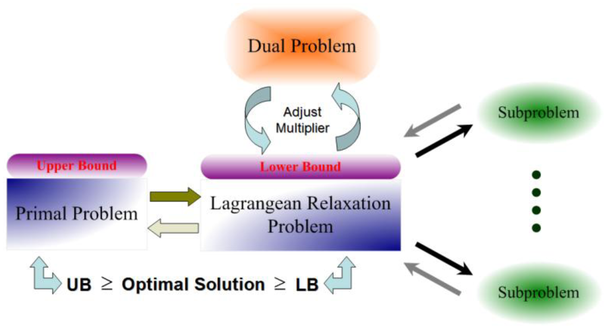
For example, if the problem is a minimization problem, the optimal value of the relaxed constraints is always a lower bound on the optimal value of original problem under the relaxed conditions. The lower bound can be improved by adjusting the set of multipliers iteration by iteration to reduce the gap of the solution between the primal problem and the Lagrangian Relaxation. This procedure is also called the Lagrangian Dual problem.

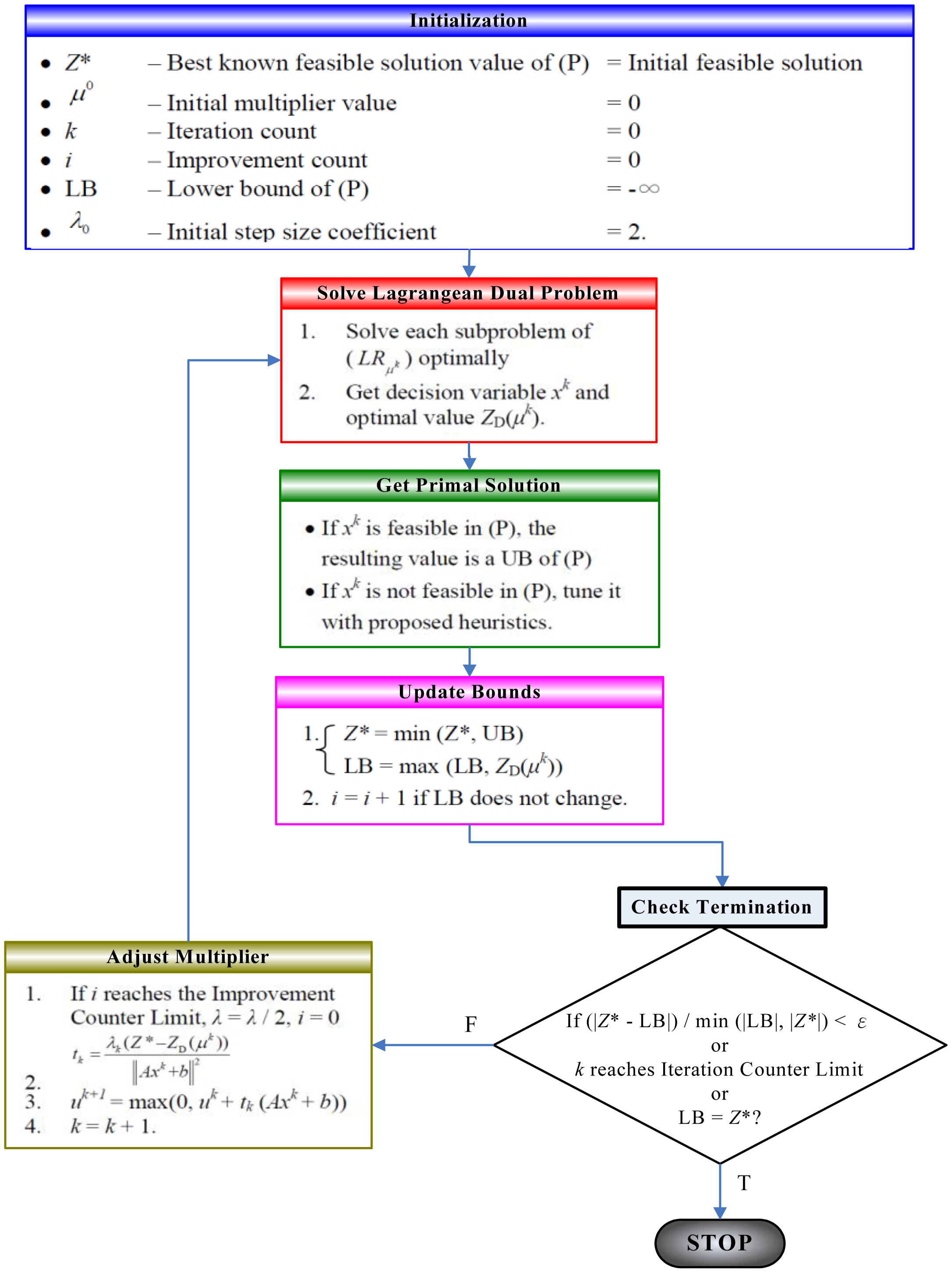
Figures 2 and 3 illustrate the underlying idea of the Lagrangian Relaxation Method, respectively. The Lagrangian Relaxation of the primal problem is developed to be a lower bound of the optimal value for the original minimization problem because some constraints of the original problem are relaxed. Therefore, it can be used as the boundary to design heuristic algorithms to get the primal feasible solution. The Subgradient Optimization Method can be utilized to minimize the gap between the primal problem and the Lagrangian Relaxation problem; this can be done through deriving the tightest lower bound by adjusting the multipliers for each iteration and then updating them to improve results.

4. Solution Approach

The solution approach to the problem formulation is based on Lagrangian Relaxation. Constraints (IP 1), (IP 3) and (IP 5) are relaxed and multiplied by nonnegative Lagrangian multipliers, ${\mu }_w^1$, ${\mu }_l^2$, _and${\mu }_{wl}^3$, respectively. They are added to the objective functions as follows.

The constraints are relaxed in such a way that the corresponding Lagrangian multipliers ${\mu }_w^1$, ${\mu }_l^2$, and ${\mu }_{wl}^3$, can be relaxed to objective function. This approach is not guaranteed to have a feasible solution due to accessing a big value of γ_w into the network which will result in unsatisfactory QoS requirement to the O-D pair w.

$\begin{array}{l}{Z}_{LR}({\mu }_w^1,{\mu }_l^2,{\mu }_{wl}^3)=\hfill \\ min\text{∑}_{l\in L}{D}_l(g_l)g_l\hfill \\ +\text{∑}_{w\in W}{\mu }_w^1(\text{∑}_{l\in L}{D}_l(g_l)y_{wl}-D_w)\hfill \\ +\text{∑}_{l\in L}{\mu }_l^2(\text{∑}_{p\in P_w}\text{∑}_{w\in W}{x}_p{\delta }_{pl}{\gamma }_w-g_l)\hfill \\ +\text{∑}_{w\in W}\text{∑}_{l\in L}{\mu }_{wl}^3(\text{∑}_{p\in P_w}{x}_p{\delta }_{pl}-y_{wl})\hfill \end{array}$		(LR)
Subject to:
$\text{∑}_{p\in P_w}{x}_p=1$	∀w ∈ W	(IP 2)
$0\le g_l\le \frac{C_l}{I(l)}$	∀l ∈ L	(IP 4)
xp = 0 or 1	∀p ∈ Pw, w∈W	(IP 6)
ywl = 0 or 1	∀w ∈ W, ∀l ∈L.	(IP 7)

We use the Lagrangian Relaxation Method to relax constraints in the formulation and decompose (LR) into two independent sub-problems. In the first Sub-Problem (SP 1), the nonnegative weight is calculated as ( ${\mu }_{wl}^3+{\mu }_l^2{\gamma }_w$) on each link. The actual meaning of the multipliers ${\mu }_{wl}^3$ and ${\mu }_l^2$ are the link mean delay and the derivative of queue length, respectively; both can be derived from the solution of the problem (LR). By the problem (LR), the multiplier ${\mu }_{wl}^3$ is related to the relaxation of link selection for each O-D pair. When one unit on the decision variable of link selection is added (i.e., y_wl), it generates one unit of the corresponding mean delay as formulated in QoS constraint, but when the problem (LR) is solved, the decision variable y_wl is either 1 or 0 not only one unit, thus, the multiplier ${\mu }_{wl}^3$ is equivalent to the mean delay on the chosen link.

Besides, the link selection is based on the sum of link mean delay D_l(g_l) of each O-D pair which is weighted by ${\mu }_w^1$, that is, how much the end-to-end delay will impact the objective function (IP). Moreover, in the problem (SP 2.1′), the first step for solving it is also related to the multiplier ${\mu }_{wl}^3$ and chooses the links for each O-D pair according to $y_{wl}^{*}(g_l)={\mu }_w^1{D}_l(g_l)-{\mu }_{wl}^3=00.$ It means that whenever a link is selected for an O-D pair, the link will produce corresponding link mean delay ${\mu }_{wl}^3$ and affect the end-to-end delay constraint which is weighted by multiplier ${\mu }_w^1$ in the problem (LR).

On the other hand, the multiplier ${\mu }_l^2$ is related to the relaxation of aggregate flow over each link. The physical meaning of ${\mu }_l^2$ would be that when ${\mu }_l^2$ can be relaxed on the link flow, it will affect the objective function (IP), which means ${\mu }_l^2$ would be the sensitivity of the average number of packets over the link with respect to the aggregate flow.

A brief illustration is shown in

Table 4. Arc weight of each link.

$\begin{array}{c}\mathit{arc\; weight}=({\mu }_{wl}^3+{\mu }_l^2{\gamma }_w)\\ =\mathit{\text{link mean delay}}+\mathit{\text{derivative of queue length}}\times \mathit{\text{required traffic}}\\ =D_l(g_l)+{\gamma }_w\times \frac{\partial \left(D_l(g_l)g_l\right)}{\partial g_l}\\ =D_l(g_l)+{\gamma }_w\times \left(D_l(g_l+g_l\times \frac{\partial D_l(g_l)}{\partial g_l}\right)\end{array}$

, ${\mu }_{wl}^3$ implies the link mean delay of each link, and ${\mu }_l^2$ indicates the derivative of queue length. The term γ_w in the arc weight form represents the weighting factor between ${\mu }_{wl}^3$ and ${\mu }_l^2$ Thus, this metric consists of the link mean delay and the derivative of queue length, considers both system perspective and user perspective for our distributed routing protocol, and uses the traffic requirement of each O-D pair as the weighting factor to combine these two parameters.

Finally, The LR problem can be decomposed into independent and solvable optimization sub-problems which are developed in a sufficient way one by one. The physical meanings of multipliers are also developed and mentioned above to help us to determine relationships of the link mean delay and derivative of queue length. We can get these important parameters to derive the routing assignments in “system perspective” and “user perspective”. The detail solving steps are illustrated in the Appendix.

In following section, the computational experiments are constructed and implemented to analyze the quality of the solution approach to verify the routing algorithms correctly. The experiments are designed for analyzing the performance of WVSN, if it can be satisfied with lower average end-to-end delay and delay jitter to transmit video data by different algorithms.

5. Computational Experiments and Results

5.1. Experiment Environment

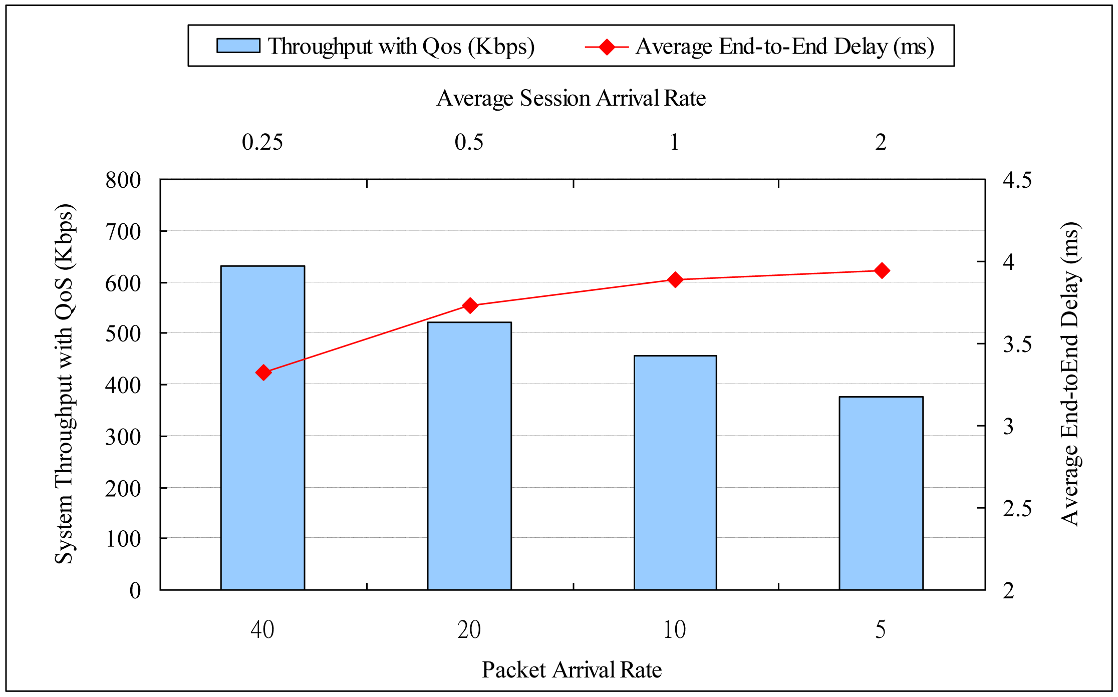
Each session follows one path for routing its required traffic emulated as a real time surveillance streaming data and is not allowed to change during the holding time. The session arrivals followed a Poisson process, and the holding time of each session is set to be an exponential distribution with average 10 s. The experiment with average session arrival rates of 0.25, 0.5, 1 and 2, and the corresponding packet arrival rates are 40, 20, 10 and 5. Figure 4 is shown as the experiment environment which QoS requirements are set in 3 × 3, 5 × 5, 7 × 7 and 9 × 9 squares in 3 ms, 4 ms, 5 ms and 6 ms, respectively.

As

Table 5. Experimental session types.

Parameters	Value
Average Holding Time	10
Average Session Arrival Rate	0.25	0.5	1	2
Average Number of Active Sessions	2.5	5	10	20
Packet Arrival Rate	40	20	10	5
Average Traffic Input	100 (packets/s)

shows, there is average of 100 packets per second in the network of each topology. The size of each transmitting UDP packet is 1,000 bytes at each packet arrival rate. Aside from the control messages of distribution routing protocol, messages such as HELLO messages for sensing the neighbors and TC message for broadcasting topology information are sent at a fixed period of 5 s.

The estimate the parameters of our routing metric (shown in

Table 6. Parameters.

Parameters	Value
Transmit and Receive Antenna Gain	1.0
Transmit and Receive Antenna Height	1.5 (m)
Reception Threshold	3.625 e−;10
Carrier Sensing Threshold	1.559 e−;11
Transmission Range	250 (m)
Interference Range	550 (m)
Distance between Each Node	200 (m)
UDP Packet Size	1,000 (bytes)
Sending Interval of HELLO Message	2 (s)
Sending Interval of TC Message	5 (s)
Recording Interval of Fitting Data	1 (s)
Number of Fitting Data	10
K	5
β	1.3

), we record each packet delay and packet inter-arrival time and then calculate mean delay and aggregate flow with corresponding queue length (i.e., average number of packets) of each link for every second. The number of data fit for power regression is set to be 10, that is, the data used to compute the regression function are the newest 10 records and the interval of each is 1 s. Additionally, the value of K in the routing algorithm is set as 5 (i.e., at most the five shortest or fastest paths for each O-D pair) and the threshold β for admission control heuristic algorithm is set to be 1.3.

If the received signal strength exceeds the reception threshold, the packet can be successfully received. If received signal strength exceeds the carrier-sensing threshold, the packet transmission can be sensed. However, the packet cannot be decoded unless signal strength surpasses the reception threshold. Both the transmission range and interference range are calculated by the two-ray ground reflection model according to the reception threshold and the carrier-sensing threshold, respectively.

This paper focuses on the effectiveness of our routing metric and related parameters at the on-line stage, and its reduction of system-wide impact between each coming session with QoS provisioning. Thus, we use a single channel in the experimental environment to decouple the effect of the channel assignment algorithm and evaluate the performance of our routing algorithm.

5.2. Performance Evaluation

In this Section, we present experimental results to demonstrate the effectiveness of our routing algorithm, NODQC. We also evaluate NODQC with other different session types of algorithms under the same average traffic loading in the network, and then compare the performance in terms of average end-to-end delay, delay jitter and system throughput with QoS satisfaction. Delay jitter is defined as the variance in the following tables and figures.

Performance evaluation is defined in

Table 7. Two-Ray Ground Reflection Model.

Transmission Range (or Interference Range)
$\sqrt[4]{\frac{\mathit{\text{TransmitPower}}\times \mathit{\text{TransmitAntennaGain}}\times \mathit{\text{ReceiveAntennaGain}}\times {(\mathit{\text{TransmitAntennaHeight}})}^2\times {(\mathit{\text{ReceiveAntennaHeight}})}^2}{\mathit{\text{Threshold}}}}$

, a 7 × 7 square is simulated as the network topology with 660 s and measure the packets at last 600 s. For comparison with other routing algorithms, we use the session types whose average session arrival rate and packet arrival rate are equal to 0.25 and 40, respectively, and use different network sizes to show the performance of NODQC, OLSR, AODV, and DSDV routing algorithms. The time of our experiment is set at 660 s and the measurement time is the last 600 s. Increasing the number of nodes will also increase the number of broadcast packets and route table updating. From

Table 8. Evaluation with different session rates (average end-to-end delay).

Average End-to-End Delay (ms)
Average Session Rate	0.25	0.5	1	2
Packet Arrival Rate	40	20	10	5
Average End-to-End Delay	3.325215	3.730487	3.88681	3.942485

and

Table 9. Evaluation with different session rates (system throughput with QoS).

System Throughput with QoS (Kbps)
Average Session Rate	0.25	0.5	1	2
Packet Arrival Rate	40	20	10	5
System Throughput with QoS	632.062518	521.353393	456.291533	376.553628

and Figure 5, the value of average end-to-end delay is shown to be increased and the system throughput with QoS is shown to be decreased with the average session arrival rate. This is because nodes exchange information every 5 s, but the sessions enter the network at a short time interval. Most sessions are consequently routed to sub-optimal paths due to a lack of updated information for the routing metric. Evaluation results indicate that our routing algorithm performs better in the lower average session arrival rate but higher packet arrival rate under the same system loading of average 100 packets per second.

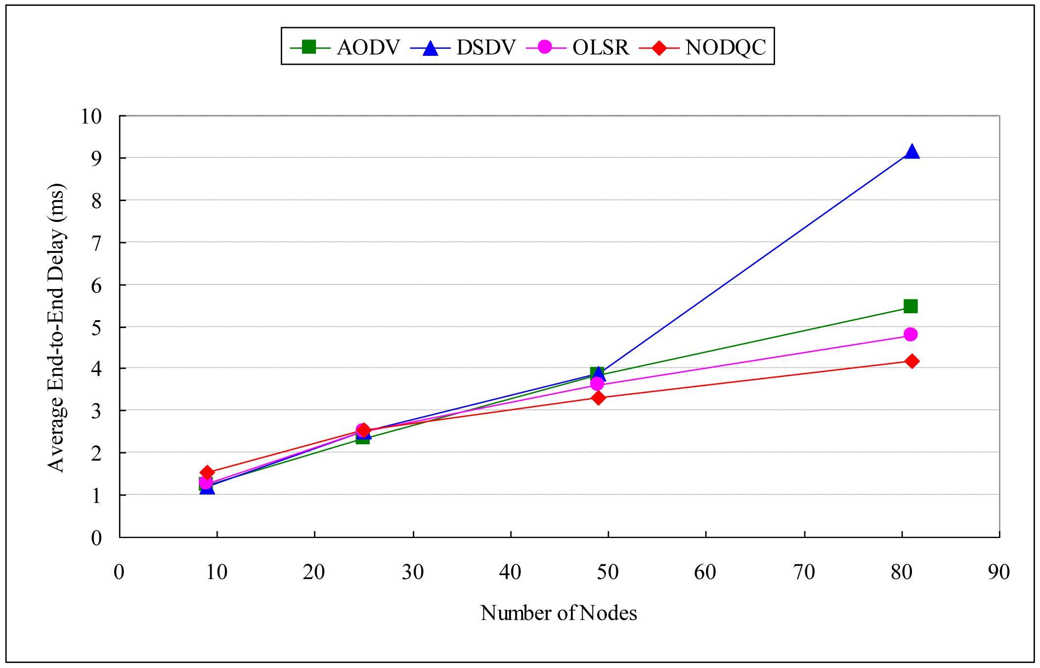
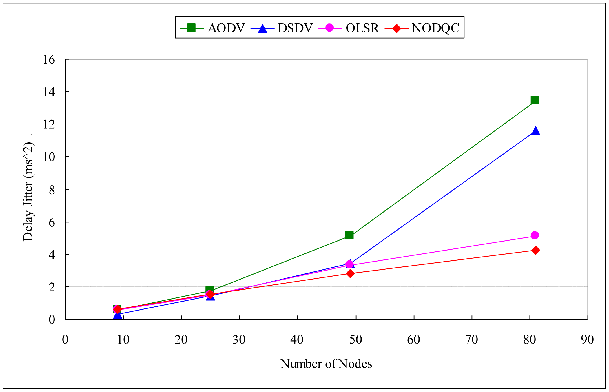
If the performance evaluation is taken in the scalability scenario, Average end-to-end delay (AE2ED) shows that it has no effect significant difference in smaller number of nodes obviously, but delay increases as the number of nodes increase.

Table 10. Experiment results of routing algorithms (average end-to-end delay).

Average End-to-End Delay (ms)
Routing Algorithms	3 × 3	5 × 5	7 × 7	9 × 9
NODQC	1.54599	2.550296	3.325215	4.176691
OLSR	1.28128	2.522533	3.620345	4.792818
AODV	1.248075	2.339906	3.848888	5.456055
DSDV	1.220291	2.495117	3.873495	9.171553

,

Table 11. Experiment results of routing algorithms (delay jitter).

Delay Jitter (ms2)
Routing Algorithms	3 × 3	5 × 5	7 × 7	9 × 9
NODQC	0.623741	1.529524	2.789917	4.239667
OLSR	0.536928	1.463894	3.332403	5.098757
AODV	0.556566	1.720252	5.129518	13.445979
DSDV	0.330232	1.418664	3.424205	11.586675

and

Table 12. Experiment results of routing algorithms (system throughput with QoS).

System Throughput with QoS (Kbps)
Routing Algorithms	3 × 3	5 × 5	7 × 7	9 × 9
NODQC	716.849085	673.698465	632.062518	612.322159
OLSR	753.008325	691.484223	603.130035	556.022380
AODV	757.683145	700.203701	575.904857	516.320711
DSDV	773.355103	701.779457	602.953338	509.221205

, Figures 6, 7 and 8 show the results of performances between different routing algorithms in each network size. In the small-scale network (e.g., 3 × 3 and 5 × 5 squares), the broadcasting of routing protocol control messages for exchanging information will causes large delays to packet transmission, especially for the destination node. Additionally, the average path length of each session is shorter in smaller networks, in which the superiority of our routing metric is not obvious.

As networks grow in size, the average path of each session lengthens with path selection becoming increasingly important. AE2ED taken in the scalability scenario shows that delay is much less for NODQC as compared to others. As routes break, nodes have to discover new routes which lead to longer E2ED (packets are buffered at the source during route discovery). According to the arc weight on each link is the combination of end-to-end delay from the user perspective and average delay from the system perspective, NODQC can choose other less or non-congested paths for the sessions and balance network-wide the traffic loading. This makes the routing strategy more flexible for making routing decisions for new routing constructions. As far as delay is concerned, NODQC performs better than OLSR, AODV, and DSDV with large numbers of nodes.

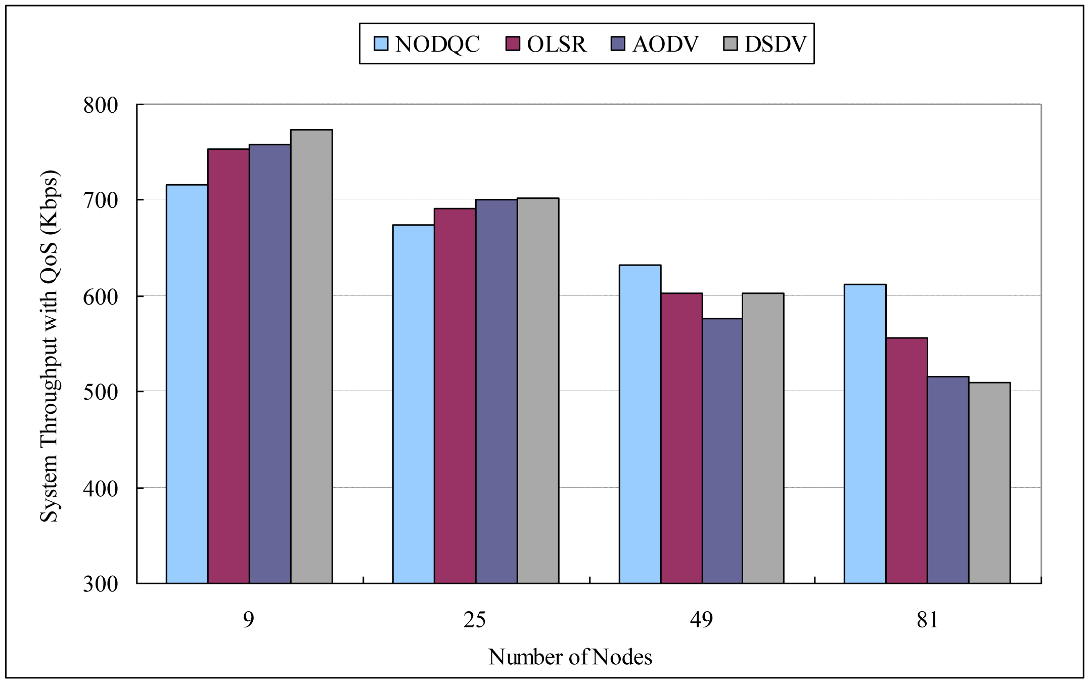
Hence for real time traffic, NODQC is preferred over OLSR, AODV, and DSDV. This is significant for the fact that, as the variations of packet delay becomes more predictable, the routing mechanisms can factor in that delay to determine whether a packet is lost or not. Furthermore, the NODQC also takes QoS provisioning into account for the coming sessions, thereby causing system throughput with QoS satisfaction to be greater than others in larger networks. By taking into consideration both the perspective of the system as we as well as users, the NODQC has proven itself to have lower average end-to-end delay and delay jitter and higher system throughput with QoS satisfaction than other routing algorithms in large-scale networks.

By leveraging the Lagrangian Relaxation method, the arc weight on each link can be applied by our routing metrics. It can employ the link-state routing protocol to construct the shortest or shorter paths within an acceptable delay. Within larger networks, routing strategies can be played to improve system performance with lower average end-to-end delay and delay jitter than alternative algorithms (OLSR, AODV, DSDV). NODQC outperforms them in terms of system throughput with QoS satisfaction.

6. Future Work

One of the most important parts of this paper is the routing metric and relevant parameters. The Lagrangian Relaxation formulations are applied to the arc weight and to infer the actual meaning of the corresponding multipliers. In addition, Lagrangian multipliers and Karush-Kuhn-Tucker Conditions can be used to succinctly describe the arc weight form. This simplifies the process of inference and has the same consequence with Lagrangian Relaxation.

Through the solution of the Lagrangian Relaxation formulation, various QoS requirements can be implemented for different purposes or services. The end-to-end delay is presented as a function in our formulation to be the QoS consideration. Distinct QoS metrics (e.g., delay jitter or packet loss rate) can be applied to the Lagrangian Relaxation formulation, and the corresponding multiplier of the routing metric, link mean delay will be replaced by the newly defined QoS metric.

7. Conclusions

In wireless visual sensor networks for real time video surveillance, sensor nodes need to be forwarded the packets to the sinks within an acceptable delay under limited resource constraints, including embedded vision processing, data communication, battery energy issues. It is a challenging issue since it needs to meet the end-to-end delay for each application and at the same time optimize the system resource utilization by minimizing the average system delay so that more real-time applications could be granted in the future. By leveraging the Lagrangian Relaxation method, the arc weight on each link is the combination of end-to-end delay from the user perspective and average delay from the system perspective. Thereafter, our routing metric employs the link-state routing protocol to construct shortest paths within an acceptable delay. Within larger networks, the superiority of the Near-Optimal Distributed QoS Constrained (NODQC) routing algorithm is more visible as path selection plays a more important role. Experimental results show that, and especially so in large-scale networks, the NODQC not only has lower average end-to-end delay and delay jitter than alternative algorithms (OLSR, AODV, DSDV) but also outperforms them in terms of system throughput with QoS satisfaction. In WVSNs for video surveillance, video coding/compression that has low complexity, produces a low output bandwidth, tolerates loss, and consumes as little power as possible is required. Our routing strategies can be applied well in a large scale network with more efficiency and effectiveness.

References

- Hadjiconstantinou, E.; Christofides, N. An efficient implementation of an algorithm for finding k shortest simple paths. Networks 1999, 34, 88–101. [Google Scholar]
- Charfi, Y.; Canada, B.; Wakamiya, N.; Murata, M. Challenging issues in visual sensor networks. IEEE Wirel. Commun. 2009, 16, 44–49. [Google Scholar]
- He, Y.; Lee, I.; Guan, L. Distributed algorithms for network lifetime maximization in wireless visual sensor networks. IEEE Trans. Circuits Syst. Video Technol. 2009, 19, 704–718. [Google Scholar]
- Misra, S.; Reisslein, M.; Xue, G. A survey of multimedia streaming in wireless sensor networks. IEEE Commun. Surv. Tutor. 2008, 10, 18–39. [Google Scholar]
- Soro, S.; Heinzelman, W. A survey of visual sensor networks. Adv. Multimed. 2009, 2009, 1–21. [Google Scholar]
- Badia, L.; Erta, A.; Lenzini, L.; Zorzi, M. A general interference-aware framework for joint routing and link scheduling in wireless mesh networks. IEEE Netw. 2008, 22, 32–38. [Google Scholar]
- Raniwala, A.; Gopalan, K.; Chiueh, T.C. Centralized channel assignment and routing algorithms for multi-channel wireless mesh networks. ACM Mob. Comput. Commun. Rev. 2004, 8, 50–65. [Google Scholar]
- Kyasanur, P.; Vaidya, N.H. Routing and Interface Assignment in Multi-Channel Multi-Interface Wireless Networks. IEEE Wireless Communications and Networking Conference, New Orleans, LA, USA, 13–17 March 2005; pp. 2051–2056.
- Subramanian, A.P.; Gupta, H.; Das, S.R. Minimum Interference Channel Assignment in Multi-Radio Wireless Mesh Networks. Proceedings of 4th Annual IEEE Communications Society Conference on Sensor, Mesh and Ad Hoc Communications and Networks, San Diego, CA, USA, 18–21 June 2007; pp. 481–490.
- Draves, R.; Padhye, J.; Zill, B. Routing in Multi-Radio, Multi-Hop Wireless Mesh Networks. Proceedings of 10th Annual International Conference on Mobile Computing and Networking, Philadelphia, PA, USA, 26 September–1 October 2004; pp. 114–128.
- Liu, T.; Liao, W. Capacity-Aware Routing in Multi-Channel Multi-Rate Wireless Mesh Networks. Proceedings of IEEE International Conference on Communications, Istanbul, Turkey, 11–15 June 2006; pp. 1971–1976.
- Tzeng, Y.C. Backhaul Assignment and Routing Algorithm with End-to-End QoS Constraints in Wireless Mesh Networks. MS.c. or Ph.D. Thesis, Department of Information Management, National Taiwan University, Taiwan, 2006. [Google Scholar]
- Cheng, H.T.; Zhuang, W. Joint power-frequency-time resource allocation in clustered wireless mesh networks. IEEE Netw. 2008, 22, 45–51. [Google Scholar]
- Alicherry, M.; Bhatia, R.; Li, L. Joint Channel Assignment and Routing for Throughput Optimization in Multi-Radio Wireless Mesh Networks. Proceedings of the 11th Annual International Conference on Mobile Computing and Networking, Coldgue, Germany, 28 August–2 September 2005; pp. 58–72.
- Mohapatra, S.; Kanungo, P. Performance analysis of AODV, DSR, OLSR and DSDV routing protocols using NS2 Simulator. Proced. Eng. 2012, 30, 69–76. [Google Scholar]
- Forouzan, B.A. Data Communication and Networking, 3 ed; McGraw Hill: New York, NY, USA, 2003. [Google Scholar]
- Tang, J.; Xue, G.; Zhang, W. Interference-Aware Topology Control and QoS Routing in Multi-Channel Wireless Mesh Networks. Proceedings of the 6th ACM International Symposium on Mobile Ad Hoc Networking and Computing, Urbana-Champaign, IL, USA, 25–28 May 2005; pp. 68–77.
- Wasiq, S.; Arshad, W.; Javaid, N.; Bibi, A. Performance Evaluation of DSDV, OLSR and DYMO Using 802.11 and 802.11 p MAC-Protocols. Proceedings of IEEE 14th International Multitopic Conference, Karachi, Pakistan, 22–24 December 2011; pp. 357–361.
- Ade, S.A.; Tijare, P.A. Performance comparison of AODV, DSDV, OLSR and DSR routing protocols in mobile ad hoc networks. Int. J. Inf. Technol. Knowl. Manag. 2010, 2, 545–548. [Google Scholar]
- Kumawat, R.; Somani, V. Comparative Analysis of DSDV and OLSR Routing Protocols in MANET at Different Traffic Load. Proceedings of 2011 International Conference on Computer Communication and Networks, Maui, HI, USA, 3 July–4 August 2011; pp. 34–39.
- Tripathi, K.; Agarwal, T.; Dixit, S.D. Performance of DSDV protocol over sensor networks. Int. J. Next Gener. Netw. 2010, 2, 53–59. [Google Scholar]
- Yen, H.H.; Lin, F.Y.S. Near-Optimal Delay Constrained Routing in Virtual Circuit Networks. Proceedings of Twentieth Annual Joint Conference of the IEEE Computer and Communications Societies, Anchorage, AK, USA, 22–26 April 2001; pp. 750–756.
- Kleinrock, L. Queueing Systems; Wiley-Interscience: New York, NY, USA, 1976. [Google Scholar]
- Wen, Y.F. Performance Optimization Algorithm for Wireless Networks. MS.c. or Ph.D. Thesis, Department of Information Management, National Taiwan University, Taiwan, 2007. [Google Scholar]
- Gallager, R.G. A minimum delay routing algorithm using distributed computation. IEEE Trans. Commun. 1997, 25, 73–85. [Google Scholar]
- Cassandras, C.G.; Abidi, M.V.; Towsley, D. Distributed routing with on-line marginal delay estimation. IEEE Trans. Commun. 1990, 38, 348–359. [Google Scholar]
- Geoffrion, A.M. Lagrangian Relaxation and its use in integer programming. Math. Program. Study 2 1974, 2, 82–114. [Google Scholar]
- Fisher, M.L. An application oriented guide to Lagrangian Relaxation. Interfaces 1985, 15, 10–21. [Google Scholar]
- Cheng, K.T.; Lin, F.Y.S. Minimax End-to-End Delay Routing and Capacity Assignment for Virtual Circuit Networks. Proceedings of IEEE Global Telecommunications Conference, New Orleans, LA, USA, 14–16 November 1995; pp. 2134–2138.
- Fisher, M.L. The Lagrangian Relaxation Method for solving integer programming problems. Manag. Sci. 1981, 27, 10–21. [Google Scholar]
- Katoh, N.; Ibaraki, T.; Mine, H. An efficient algorithm for k shortest simple paths. Networks 1981, 12, 411–427. [Google Scholar]