
Multiple Two-Way Time Message Exchange (TTME) Time Synchronization for Bridge Monitoring Wireless Sensor Networks


1
Robot Technology Used for Special Environment Key Laboratory of Sichuan Province, Southwest University of Science and Technology, Mianyang 621010, China
2
College of Chemistry and Environment, Sichuan University of Science and Engineering, Zigong 643000, China
3
Advanced Robotics and Intelligent Systems (ARIS) Laboratory, School of Engineering, University of Guelph, Guelph, ON N1G 2W1, Canada
4
State Key Laboratory of Geohazard Prevention and Geoenvironment Protection, Chengdu University of Technology, Chengdu 610059, China
*
Authors to whom correspondence should be addressed.
Sensors 2017, 17(5), 1027; https://doi.org/10.3390/s17051027
Submission received: 5 March 2017
/
Revised: 19 April 2017
/
Accepted: 27 April 2017
/
Published: 4 May 2017
(This article belongs to the Special Issue Sensors for Transportation)
Abstract
:Wireless sensor networks (WSNs) have been widely used to collect valuable information in Structural Health Monitoring (SHM) of bridges, using various sensors, such as temperature, vibration and strain sensors. Since multiple sensors are distributed on the bridge, accurate time synchronization is very important for multi-sensor data fusion and information processing. Based on shape of the bridge, a spanning tree is employed to build linear topology WSNs and achieve time synchronization in this paper. Two-way time message exchange (TTME) and maximum likelihood estimation (MLE) are employed for clock offset estimation. Multiple TTMEs are proposed to obtain a subset of TTME observations. The time out restriction and retry mechanism are employed to avoid the estimation errors that are caused by continuous clock offset and software latencies. The simulation results show that the proposed algorithm could avoid the estimation errors caused by clock drift and minimize the estimation error due to the large random variable delay jitter. The proposed algorithm is an accurate and low complexity time synchronization algorithm for bridge health monitoring.
1. Introduction
Bridges are an important part of transportation systems, Structural Health Monitoring (SHM) of bridges is indispensable and multiple sensors such as acceleration, displacement, temperature and strain sensors [1,2,3,4,5,6] are employed to collect the real-time information about bridges. As described in [1,5,6] synchronized sensing is necessary to ensure accuracy in SHM applications, so time synchronization is a key technology in the wireless sensor networks (WSNs) used for SHM of bridges and is important for collaborative tasks, intelligent sleeping and data consistency [5,6,7,8]. WSN nodes use local hardware clock sources to set up their local times, which differ from each other. There are two main reasons for these differences. The nodes are initialized at different moments so there is clock offset among nodes. More than that, the clock sources have variable clock frequency offsets which are due to the clock manufacturing techniques used and the changing environments. Hence in networks there is clock skew and variable clock offsets. Time synchronization algorithms are proposed to correct the local time information and force the time notions of different nodes to be consistent. It has been used in many WSN applications, such as location [9,10,11,12], environmental monitoring [13,14,15,16], data acquisition [17,18,19], delay measurement [20], power saving [21] and so on.
Accurate clock offset estimation is one of the key factors to improve the time synchronization. One type of proposed time synchronization algorithms correct the clock offset between nodes [13,22,23]. These approaches provide for simple calculations and cost less to achieve, but because of the influence of the ignored clock frequency offset, these time synchronization algorithms need re-synchronization to maintain the precision. Some improved algorithms introduced joint skew-offset correction [9,22,23,24,25,26,27,28,29,30,31]. Additionally, these algorithms correct the relative clock speeds and reduce the clock skew, so the time synchronization algorithms with joint skew-offset correction are better for synchronization over a long time. Actually, almost all of the joint clock skew-offset correction time synchronization algorithms use the existing clock offset estimations to calculate the relative clock speed and compensate the clock skew. Obviously, accurate clock offset estimations are important for the clock skew estimate of time synchronization algorithms.
The early time synchronization algorithms such as RBS [21] use a large number of beacon broadcasts to synchronize a pair of receivers. The receivers record the arrival time of the beacon signals and exchange it among each other, then the clock offset and clock skew can be calculated. Absent MAC-layer timestamps, RBS provides a rough time synchronization. The improved CESP algorithm [23] introduces the reference node MAC-layer time stamp into the beacons’ broadcasts. It uses synchronization coefficient exchange instead of time information exchange and the communication overhead is reduced. TPSN [24] is a time synchronization algorithm for sender to receiver and uses rough time stamps, but its clock offset estimate error is nearly two times smaller than that of RBS.
FTSP [9] floods the reference time information to the networks and employs multiple MAC-layer time stamps to improve the time stamp precision. The flooding packets, which load the send time stamps of reference nodes, are broadcasted periodically. The receivers estimate the clock offset and skew by exchanging their time stamps directly. PulseSyn [25] is a rapid-flooding time synchronization algorithm that believes that all of the nodes should to broadcast the reference time information as soon as possible. It aims to solve the problem of the amplified error caused by the delay before a node broadcast gets its received reference time information. FCSA [26] verifies that there is a smaller time synchronization error if the nodes have less clock frequency differences. It uses a clock speed agreement algorithm to improve the slow-flooding time synchronization algorithm in FTSP. There are many other algorithms which are complete distributed time synchronization algorithms. GTSP [27] and EGSync [28] were proposed to minimize the skew of any two neighborhood nodes. The consensus-based algorithms ATS [29], MTS [30] and CCS [31] are effective for dynamic topology networks. These algorithms have slow convergence rates for accurate time synchronization. SHM of bridges is a special application of WSNs, where the traditional synchronization methods may not meet its needs and many time synchronization algorithms are proposed for the data gathering and data fusion [7,8,32,33]. Xiao et al. [32] and Hu et al. [7] focused on the energy efficiency of time synchronization, and improved the previous algorithms and proposed an energy balanced time synchronization algorithm to lengthen the whole WSNs’ life. Xu et al. [8] proposed an asymmetrical clock synchronization algorithm for bridge health monitoring WSNs to monitor real-time bridge conditions. To improve the TPSN [24] for ensuring the synchronization accuracy without consuming more power, Gong et al. [33] proposed a partial TPSN time offset synchronization scheme for bridge health diagnosis WSNs.
The transmission delay results in a large error for clock offset estimation, especially for the random variable delay portion. Specific time message exchange mechanisms are employed by time synchronization algorithms to reduce these disadvantages. WSNs are a complete distributed system. The hardware resources and computational power are limited. The clock frequency of a node could not be measured directly. Its transmission delay is unknown and variable, so the time synchronization algorithms always estimate the clock offset from time information transmissions [34,35]. One-way broadcast time messages are employed for synchronizing receiver to receiver [25,29]. The reference nodes broadcast their time information packets periodically and the receivers use the time message to correct their local times. This mechanism removes the variable delay from clock offset estimate at the sender but a variable delay is introduced into the estimation directly at the receiver.
The two-way message exchange (TTME) clock offset estimator was first proposed in TPSN [24] for wireless sensor network time synchronization. It uses pairs of transmissions that are named and to make four time stamps. Then the time stamps are used to estimate and correct the clock offset among nodes. Chaudhari et al. [36] and Wang et al. [37] employed an ACK mechanism TTME, but not a dedicated time message packet. These protocols only use the uplink time stamp for clock offset estimation. Jeske [38] proved that the MLE exists for TTME. The transmit delays were denoted as fixed portions and variable portions as decomposed by Abdel-Ghaffar [39]. To calculate the clock offset of MLE, it is assumed that there are a subset of TTME observations which have same fixed clock offset. In employing the minimum observations of uplink and downlink the clock offset of MLE can be calculated. Noh et al. [40] assumed that the probability distribution function of random variable delay was either an exponentially distribution function or a Gaussian distribution function. They proved the Cramer-Rao lower bounds (CRLBs) for the clock offset MLE under these different delay models.
However, a time synchronization scheme for WSNs in bridge health monitoring that has remarkably low complexity and ease of implementation still needs to be developed. In this paper we focus on MLE of two-way message exchange (TTME) clock offset estimation. For MLE of clock offset estimate, a sufficiently large subset of TTME observations is a prerequisite. In addition, a same fixed clock offset for the subset is beneficial for accurate clock offset estimation.
TTME like TPSN may not meet the MLE of clock offset estimation. To simplify the description, the TTME similar to TPSN is named traditional TTME. The traditional TTME ignores the random variable delay and introduces it into the clock offset estimation. Additionally, the clock offset due to the clock drift is not considered. Since the assumption that nodes have fixed clock offset is not always valid and the TTME in TPSN is an ideal clock offset estimate model, the main clock offset estimate error for these algorithms are caused by random variable delay and clock drift. Especially when there are large transmission delay jitters and large software blocking latencies, the estimate errors will increase predictably.
Our work aims to meet these requirements. The multiple TTMEs in this paper provide an effective clock offset MLE approach for time synchronization in WSNs which is a potential application for SHM of bridges. The proposed algorithm demands less calculation and is easy to embed in the WSN application. This paper takes an optimized TTME approach to achieve high precision time synchronization for the data acquisition in bridge health monitoring WSNs. We have discussed the details of the clock offset continuously increasing, then optimized the execution time and speed of the TTME to meet the assumption in TPSN. The maximum likelihood estimation (MLE) is employed to reduce the clock offset estimate errors due to the random variable delay. Then the multiple TTMEs algorithm aims to provide as many TTME observations as possible for MLE. The multiple TTMEs is different from the traditional TTME. It employs the timeout constraint to avoid the clock offset estimation errors due to the uncertain communication links and response delays caused by the task blocking latencies of software. Compared to TPSN, the proposed algorithm obtains more accurate clock offset estimations and lower clock skews.
The rest of this paper is organized as follows: in Section 2, we introduce the system model. In Section 3, we analyze the details of the continuously increasing clock offset, and derive the restraints for the fixed clock offset TTME. The multiple TTMEs algorithm is proposed in Section 4. The clock offset and clock skew estimate are described in Section 5. The simulation results are shown in Section 6 and finally, we present our conclusions in Section 7.
2. System Models
In this section, we introduce the system models that are used in our work. The bridge monitoring WSN model is defined as a graph, . The subset of nodes is defined as . The bidirectional communication link (edge) subset is defined as . An arbitrary node has a neighborhood nodes subset and node can only communicate with the nodes in . The distance between arbitrary nodes is defined as the number of edges on the shortest path between the two nodes. The diameter is defined as the maximum distance of any two nodes in the graph .
2.1. Time Synchronization for SHM of Bridges
Based on the shape of bridges, the topology of bridge monitoring WSNs can be designed as a spanning tree [1], so the time synchronization algorithm employs the tree to maintain the time synchronization. The MAC layer time-stamping technology is employed to make time stamps. Root is the reference node and starts the TTME to force its child nodes to synchronize to itself firstly. Then the synchronized nodes become reference nodes and start the new TTME to synchronize their child nodes until the network has synchronized the end node along the spanning tree.
The architecture of time synchronization for SHM of bridges is shown in Figure 1. It assumes that a spanning tree is created. The root of the tree is the reference node of the network, which employs GPS as an external clock source. The routers are forwarding nodes for the time synchronization. The high level nodes always employ their parent as reference node and synchronize to it. After the spanning tree is created, the root initializes the time synchronization by an initialization broadcast. The router node, which has received this broadcast, is synchronized to the root, and then sets itself up as a reference for its own nodes. The router uses two steps to flood the time synchronization through the network: (1) it requests a synchronization response from the reference node to estimate the clock offset and clock skew; (2) it compensates the local clock source parameter, and then transforms itself into the reference node of its son nodes and initializes the synchronization.
2.2. Clock Model
The bridge monitoring WSN nodes are driven by hardware clock sources which usually are crystal oscillators. The time notion is created by counting the hardware clock pulses. The clock speed of the node is the increment of its time count in the specified time range, i.e., . is the time counting of node at time , and is defined as:
If is the nominal frequency of hardware clock in node , then the granularity of the time counter is . The time notion of the node can be defined as:
is the logic time of node at time . is the logic time of node at time and it is the initial time of node . If is the moment that the nodes synchronize to each other, then the relative time model and clock offset model of pairs nodes and are defined as:
where and are logic time of and at time . is the clock offset between and at time . The is defined as the time synchronization error.
For the arbitrary node and arbitrary node , the local skew is defined as the maximum relative clock offset between nodes and at time , i.e., . For the arbitrary node , the global skew is the maximum relative clock offset between nodes and at time , i.e., . The time synchronization algorithm is employed to enforce .
2.3. TTME Clock Offset Estimation Model
To simplify the description, is defined as the reference node and is defined as an asynchronous node. The details of traditional TTME are shown in Figure 2. The node needs to be synchronized. is the reference node. The TTME has two steps. In the first step, sends a short message to . This message is just filled with the identity number of nodes and . Once the message is sent successfully, will create a local logic time stamp . The node will make the local logic time stamp after the message is received. This step aims to create time stamps and and is defined as . The second step is . The reference node respond with the TTME at . sends another short message which contains the time stamps and to . Node records the time of the message arrival as time stamp . This step aims to create time stamps and . is the duration time for TTME uplink, i.e., . is the duration time for TTME uplink, i.e., . is defined as the fixed transmission delay between and . and are the variable transmission delay. and are the clock offset of relative to .
is the time interval between and on node . It is the duration time of TTME. . The is the time interval between and on node . It is the response delay of TTME. . is a variable latency from software delay, such as the interrupt response delay, priority queuing delay, software blocking latencies. Furthermore, . and are described as the random variable with exponential distribution. For this reason we assume that is random and variable with exponential distribution, and the mean is unknown.
Traditional TTME clock offset estimation is given by Equation (5). There is clock offset for the TTME and among nodes ascribed to the clock frequency offset. . and are relative clock offset for node during TTME.
Equation (5) can be rewritten as:
where is the clock offset at the beginning of TTME between node and . is the estimation for . TTME time synchronization uses to correct the local logic time instead of . Equation (6) shows that estimate errors are mainly caused by , and .
The TTME uses time stamps to estimate the clock offset, so it is necessary to discuss the time stamping method. For different approaches, there are differences in the precision of time stamps. RBS creates the time stamp at the application layer and an uncertainty delay at the sender is introduced into the time stamp. TPSN creates its time stamping at the MAC-layer when the packet is about to be transmitted. This reduces the error caused by any uncertainty delay. FTSP uses multiple MAC-layer time stamps which were created by bytes transmission and alignment to reduce the jitter of time stamping. The multiple MAC-layer time stamps approach can obtain a higher precision time stamp so it is also employed by this paper.
3. Preliminaries for TTME Clock Offset Estimate
The proposed algorithm has proven that is not equal to and special probability distribution functions are employed to estimate them [39]. Additionally, is not equal to and is not equal to zero. In this Section, we analyze the details of clock offset changing and then the multiple TTMEs method is proposed to create the subset of fixed clock offset observations for MLE.
3.1. Increasing Clock Offset
The clock source of bridge monitoring nodes is usually driven by a rough crystals oscillator. The max frequency offset could be up to dozens of ppm or even hundreds of ppm. If the clock frequency offset is relatively stable in a short time then the clock offset increase speed is fixed, the max clock offset can be calculated.
Assume that the frequency of nominal clock source is . The frequency offset of the arbitrary clock source is ppm. . The frequency of clock source can be rewritten as in Equation (7). Both and are unknown:
in Equation (8) is the timing granularity of node . It is the ideal clock period for a logic time counter but not the real period of clock . When set the angular rate , the real time phase is . The real time phase difference between and can be written as:
where is the phase of at . is the phase of at . in Equation (10) is the counts of differences for compared to at time t. The in Equation (11) is the relative clock offset model of node . The reference clock is . is a continuous clock offset for the hardware clock.
In short, the clock offset is increasing continuously. is the increasing speed of clock and is due to the frequency offset, so there is variable clock offset in TTME. The estimate errors of clock offset in Equation (6) are unavoidable.
3.2. Fixed Clock Offset for Logic Time
The fixed clock offset does not exist in the hardware clock, but in logic time notion. Nodes employ a counter or timer to set up the logic time. This time notion is not a continuous time but a discrete time which increases by an integer multiple time of granularity . We define as the logic time of node . is the clock pulse count of at . is the actual period of clock . Then we can write as:
The time granularity of logic time is , but not the period and . is rounded down . The logic time is a discrete representation of the real time . By rewriting Equations (10) and (11), we have the logic time offset of nodes and given as:
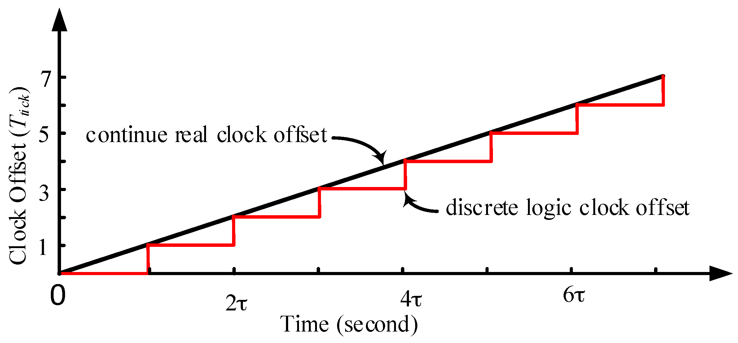
where is the number of cycles difference between nodes. is the logic time offset of nodes and . The logic time offset is different from hardware clock offsets. As Equations (14) and (15) show, and are variable. For the fixed , the larger clock frequency offset leads to larger clock offset. If , in a bounded time :
Assumption 1.
If the increment of is not larger than 1 , then there is a fixed logic clock offset .
The logic time offset is gradually increasing as shown in Figure 3. In the period that is non-integer, is a fixed value. The TTME clock offset is but not
Therefore the fixed clock offset for TTME exists with restrictions. As Figure 3 shows, the logic time offset is a discrete integer multiple time granularity so that at the range of and (), there is a fixed logic clock offset. When there is phase offset among the clock sources, the valid pulse edge for different clock sources arrives at the time counter alternately, so there is an unavoidable clock offset of less than . If the valid pulse edge of arrives ahead and the clock offset is , the clock offset is when the valid pulse edge of arrives. This will reduce the precision of clock offset estimation and intensify the clock skew.
4. The Multiple TTMEs for Time Synchronization
Based on the above analysis the estimate error of Equation (6) is given by . The define the time stamp of TTME as the time origin, set while for the logic time notion the clock offset increment is given by but not , so . Based on Assumption 1 the clock offset model is given by:
where is the time cost that the clock offset increment grows from zero to one . As Equations (14), (15) and (18) show, for a shorter , there is the greater probability that equal to in Equation (13) and the smaller estimate error for . So if , . Set , and , Equation (15) can be rewritten as:
where in Equation (19) will satisfy Equation (18). If the cost time of TTME is less than , then its observations has a fixed clock offset. is the relative frequency offset between and .
The multiple TTMEs are proposed based on TTME. Firstly, we need to calculate the which is the time cost for the increase in one. If , and, Equation (11) can be rewritten as:
For a known , is determined by . As shown by Equation (18), the time cost of the local clock offset increment is smaller than one when the time cost is smaller than in Equation (20), so the TTME observations at the period of have the same fixed clock offset which is defined as .
The multiple TTMEs algorithm is proposed to establish times TTME at the period and obtain the TTME observations set . is the variable delay of uplink for the TTME . is fixed delay of downlink for the TTME . is the time stamps for the TTME . is the time cost for the times TTME, . is the expectation of multiple times for multiple TTMEs, i.e., the number of observations (). It is important parameter for multiple TTMEs time synchronization algorithm and should be set as constant. The multiple TTMEs are defined as Algorithm 1.
| Algorithm 1. Multiple TTMEs with timeout constraint |
| ■ Initialization |
| 1. set . |
| 2. set , . |
| ■ TTME |
| 3. run the Two-way message exchange. |
| 4. . |
| 5. . |
| ■ Timeout detection |
| 6. , . |
| 7. if then jump to 3. |
| 8. . |
Multiple TTMEs employ as time out restraint (). determines the times of TTME. The is and . The temporary variable is used to record the number of valid observations. TTME is repeated until there is timeout (). Timeout detection is employed to guarantee the TTME observations to have the same fixed clock offset (). The details of the multiple TTMEs protocol are shown in Figure 4. The observations , . The fixed clock offset is:
The estimation for is , , Equation (21) is rewritten as:
Compared to Equations (6) and (15), the observations satisfy Equation (22) when . According to Equation (19), there is a larger for the smaller clock frequency offset Then there is a larger expectation for the multiple TTMEs number so that it is more reliable to estimate the delay with a distribution function. The multiple TTMEs guarantee a same fixed clock offset for the time stamps and aim to obtain an observation set as large as possible. The clock offset estimate error for is mainly due to the random variable delay and .
The constant needs to be set at an appropriate value. A smaller leads to a smaller and a tighter restriction for timeouts. There will be a smaller for a reliable TTME so that the TTME has greater probability of getting a fixed clock offset for time stamps and higher precision of clock offset estimation for time synchronization. Conversely, a larger means that there is a loose constraint for TTME. The probability for the fixed clock offset time stamps is smaller. There will be rough clock offset estimation for TTME. In addition, does not only determine the precision of clock offset estimation, but also relates to the efficiency of time synchronization. A tight timeout restriction leads to a greater probability of TTME retries (Algorithm 1, line 7), and can even lead the TTME into an infinite loop (Algorithm 1, line 7), so a maximum retry number should be employed to avoid this worse case. Therefore, an exact will balance the accuracy and convergence speed of time synchronization algorithm. A big makes the TTME of Equation (5) invalid. The multiple TTMEs hold the and avoids the additional error .
5. The Clock Offset and Clock Speed Correction
The multiple TTMEs aim to correct the relative clock offset and clock speed. The clock offset estimation refers to the precision of time synchronization, while the clock speed estimation refers to the clock skew for networks.
is defined as the time relative clock offset estimation at node . is defined as the relative clock speed offset at for node . is the estimation for . The root node has .
| Algorithm 2. MLE clock offset and linear regression clock speed, if is not , is reference node for . |
| ■ Initialization |
| 1. set . |
| 2. set , . |
| 3. receive and save . |
| ■ Clock offset MLE |
| 4. load . |
| 5. . |
| 6. . |
| ■ Linear regression clock speed |
| 7. if then then jump to 12. |
| 8. else load . |
| 9. . |
| 10. = , . 11. broadcast , correct clock speed. 12. quit. |
The term provides the global reference clock. Both the clock offset correction and clock skew compensation of the time synchronization algorithm are used to force the logic time between node and to be consistent. In the initialization period of multiple TTMEs, is defined as a counter to record the number for clock offset estimation (). The constant is employed to limit the number of MLE observations (). is the relative clock speed offset estimation for . Once node estimates the successfully, it broadcasts a time synchronization packet which is filled with immediately (). The clock offset MLE is initialized once multiple TTMEs are finished. The clock offset estimations are recorded as the set of observations for clock speed offset estimate (). The clock speed offset is calculated once the set of is big enough (). The relative clock speed offset is the sum of and (). Node employs to compensate its local clock speed to root , at the same time the is broadcasted to help its son nodes to correct clock speed offset ().
5.1. MLE Clock Offset Estimation
The MLE for clock offset with unknown fixed delay is proven by Jeske [38]. The random variable delay and are described as an exponential distribution. The CRLBs of MLE is proven by Noh et al. [40]. The clock offset MLE is given by [38]:
where is the MLE for clock offset. Its CRLBs is given by [40]:
where is defined as the mean of and , is number of times for TTME, and also is number of observations. The mean square errors (MSEs) of clock offset estimation under exponential distribution are shown in Figure 5.
As the TTME observations increase, the MLE achieves a higher precision for clock offset estimation. The traditional time synchronization algorithms like TPSN yield rough clock offset estimations, while the clock offset estimations error of MLE are reduced as the TTME observations increase. The MSEs of MLE fall faster and closer to the CRLB.
If there is the largest probability to satisfy the implicit premise that all the observations have the same fixed clock offset, so the number of observation is limited by and the speed of TTME. The proposed multiple TTMEs algorithm maximizes the by optimizing the TTME. The improvement of multiple TTMEs for clock offset MLE is shown in Figure 6.
5.2. Linear Regression Clock Speed Estimation
The clock offset correction is just to force nodes to have a consistent logic time at the correction time. While the of nodes based on the clock frequency offset is different, these nodes get different at the time range , so the clock offset is continuously changing and clock skew is introduced. Many time algorithms employ resynchronization to restrain the skew but this is not efficient for WNS, so clock speed correction is important and efficient to optimize the clock skew for WSN time synchronization protocols.
We use the latest observations of clock offset estimation to estimate the clock speed. The least squares method is used to regress these observations. The slope of the regression function is the clock speed offset . There is jitter for the clock frequency and the jitter is caused by the environment changes. We assume that the clock frequency offset and is fixed for a limited time. Equations (25) and (26) are the models for the clock offset and clock speed:
is the MLE for the relative clock offset between node and at time. is the local time of node estimating clock offset, i.e., the time stamps . is the reference node, if = 1, . If and the clock speed of node is faster than , node should speed up . If and the clock speed of node is slower than , node should slow down . is speed correction coefficient and the logic clock of could be rewritten as:
The clock speed correction coefficient of node is given by Equation (28). The algorithm employs to optimize the local clock speed , and aims to make node and have the same clock speed.
should be set at an appropriate value. A small leads to a small subset of clock offset estimate observations for linear regression. The clock offset estimate error of any observation will introduce a larger error into the clock speed offset estimation. Although more clock offset estimate observations lead to a better linear regression, a long time is needed to collect these observations, so it is not efficient. Even worse, if the environment is changing during this period, the relative clock speed is never fixed and continuously changing, so linear regression is unusable.
6. Simulation Results and Discussion
A simulation platform based on the True-Time 2.0 toolbox was established to perform the experiment. As we have discussed, TPSN is a typical traditional TTME algorithm, we compared the performances of our algorithm with TPSN. We set the hardware clock frequency as , ppm the clock drift as ppm. For both traditional TTME in TPSN and the multiple TTMEs the statistical properties were compared.
The line model with five nodes was established. The nodes identification numbers were set as 1 to 15. The networks topology was set as line . Node 1 was root and in the middle of bridge. , , . The interval of re-synchronization was 20 s. Both the interrupt handling delays of sender and receiver were random variables value with an exponential distribution, .
6.1. The Synchronization Error
The accuracy clock offset estimation is the important factor for both setting up time synchronization and holding that time synchronization. The time synchronization is set up by correction of and of . The accurate clock offset estimations are important for an efficient bridge monitoring WSN time synchronization algorithm.
For arbitrary and (), the synchronization error . Its max estimate error . The average estimate error is . Figure 7 show that the max error of traditional TTME is . Figure 8 show that the max error of multiple TTMEs algorithm is , we set a small value for so that the max estimate error caused buy clock drift is a single , i.e., , while the time synchronization error is mainly caused by and . The multiple TTMEs for MLE clock offset estimate reduce the error efficiently.
The average error of traditional TTME is about , the standard deviation of its estimation error is . The average error of multiple TTMEs algorithm is about , the standard deviation of its estimation error is . The other statistical property shows in Table 1. The probability for the multiple TTMEs algorithm that the time synchronization error is smaller than is 95 percent, while the probability for traditional TTME is 32 percent, so the multiple TTMEs algorithm is better to restrict the estimate errors caused by variable delays.
Since the ideal clock source granularity (clock source period), as discussed in Equations (12) and (13), it’s reasonable that if the hardware clock offset is less than one it is difficult to estimate this clock offset. Figure 9 shows the MSE of an average clock offset estimation. Because of the increasing number of observations, the MSE is significantly smooth. It shows that the multiple TTMEs algorithm is better than traditional TTME.
6.2. The Clock Skew
The clock offset estimate error is always introduced to the clock speed estimation and manifests as clock skew. To restrain the clock skew could improve the precision of synchronization and extend its hold time. To get a long time synchronization without frequently resynchronizing, it’s an efficient way to employ an accurate clock speed estimation to restrain the clock skew.
The multiple TTMEs algorithm provides a more accurate clock offset estimate and the clock skew estimation error needs to be discussed. We have simulated the clock speed estimate efficiency of traditional TTME and multiple TTMEs. Figure 10 shows the convergence rate. The multiple TTMEs algorithm is faster and smoother. The multiple TTMEs algorithm needs fewer observations to obtain a higher precision clock speed estimation, it has more advantages for the WSN time synchronization applications with poor storage and calculation ability.
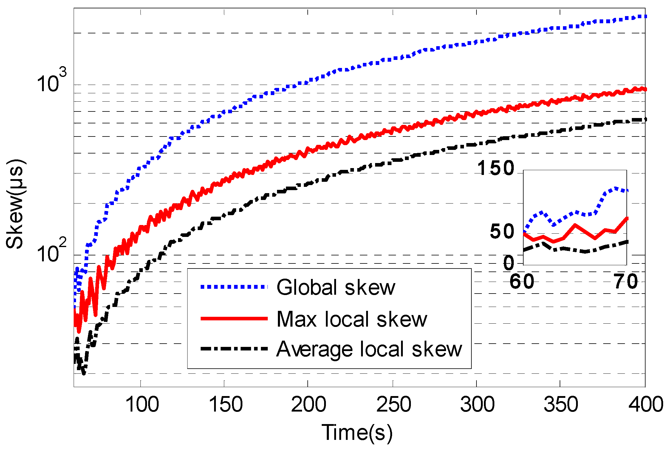
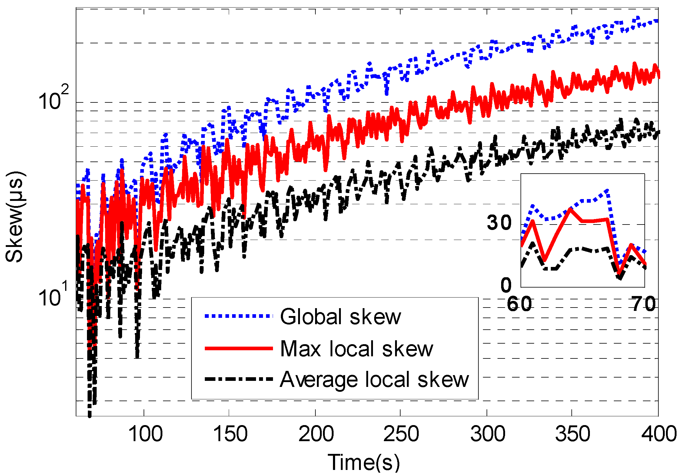
The clock skew could be reduced visibly when the time synchronization algorithm employs clock speed compensation. Figure 11 and Figure 12 show the local clock skew and global skew for traditional TTME and multiple TTMEs. The first is the initialization period for time synchronization. The accurate estimation is due to the high precision clock offset estimation and it will minimize the clock skew. The local skew of multiple TTMEs algorithm is better than traditional TTME. The skew of the multiple TTMEs algorithm is smaller than that of traditional TTME.
As the local skew increases, the global skew will inevitably increase. Since the max frequency offset is , if the time synchronization algorithm has no clock skew estimation, the global skew increasing rate is up for every 60 by Equation (11).
The global skew of traditional TTME increases at the speed nearly for every . The average speed of local skew increase for traditional TTME is nearly for every , and the max speed is near for every .
The global skew of the multiple TTMEs algorithm increases at a slower rate, as the speed is nearly for every . The speed of increase of the local skew for the multiple TTMEs algorithm is lower also, as the average value is near for every , and the max value is nearly for every .
7. Conclusions
This paper presents an easy method for MLE time synchronization for bridge monitoring wireless sensor networks. Various sensors are employed for sensing the real-time information of a bridge and these sensors are deployed on the bridge in the wireless bridge monitoring system, so a same time notion is important for multiple sensor data fusion. Time synchronization algorithms aim to build a consistent time notion. The proposed time synchronization algorithm promises an effective observations set for MLE. We have discussed the error sources of TTME clock offset estimation and details of different clock offset models. Based on the important assumption that there is fixed offset for TTMEs, a multiple TTMEs mechanism is proposed to guarantee this assumption. With multiple TTMEs, an observation set which has fixed offset can be created to meet the clock offset MLE. The simulation results show that compared to traditional TTME algorithms like TPSN, the multiple TTMEs algorithm can achieve a higher time synchronization precision. The algorithm uses a hierarchical topology spanning tree to build time synchronization quickly in the networks. As Tomonori, and Spencer [1] discussed, it is acceptable for SHM that the time synchronization error be smaller than a millisecond, so the proposed approach in this paper is suitable for bridge SHM.
Further evaluation of our protocol is needed. While there is large random latency in the node response process, the communication cost of multiple TTME retries should be considered. The timeout parameter should be optimized to make the time synchronization algorithm converge fast.
Acknowledgments
This work was supported by National Natural Science Foundation of China (Grant No. 61601383, 41227802, 41604088). This work was also supported by National Defense Pre-Research Foundation of China (Grant No. B3120133002).
Author Contributions
Fanrong Shi designed the algorithm and simulation model, wrote the paper. Xianguo Tuo helped analysis the clock model and the clock offset increasing rule of hardware clock. Huailiang Li helped performing the simulation model. Simon X. Yang helped the designing of algorithm and the writing of this paper. Rui Shi helped the data analysis and figure plotting.
Conflicts of Interest
The authors declare no conflict of interest.
References
- Nagayama, T.; Spencer, B.F., Jr. Structural Health Monitoring Using Smart Sensors; Newmark Structural Engineering Laboratory, University of Illinois at Urbana-Champaign: Urbana-Champaign, IL, USA, 2007. [Google Scholar]
- Xiong, C.; Lu, H.; Zhu, J. Operational Modal Analysis of Bridge Structures with Data from GNSS/Accelerometer Measurements. Sensors 2017, 17, 436. [Google Scholar] [CrossRef] [PubMed]
- Chen, Z.-S.; Zhang, C.; Wang, X.; Ma, C.-M. Wind Tunnel Measurements for Flutter of a Long-After body Bridge Deck. Sensors 2017, 17, 335. [Google Scholar] [CrossRef] [PubMed]
- Chae, M.J.; Yoo, H.S.; Kim, J.Y.; Cho, M.Y. Development of a wireless sensor network system for suspension bridge health monitoring. Autom. Constr. 2012, 21, 237–252. [Google Scholar] [CrossRef]
- Jang, S.; Jo, H.; Cho, S.; Mechitov, K.; Rice, J.A.; Sim, S.H.; Jung, H.J.; Yun, C.B.; Spencer, B.F., Jr.; Agha, G. Structural health monitoring of a cable-stayed bridge using smart sensor technology: Deployment and evaluation. Smart Struct. Syst. 2010, 6, 439–459. [Google Scholar] [CrossRef]
- Rice, J.A.; Mechitov, K.; Sim, S.H.; Nagayama, T.; Jang, S.; Kim, R.; Spencer, B.F., Jr.; Agha, G.; Fujino, Y. Flexible smart sensor framework for autonomous structural health monitoring. Smart Struct. Syst. 2010, 6, 423–438. [Google Scholar] [CrossRef]
- Hu, X.; Wang, B.; Hu, X. A Novel Energy-Balanced Time Synchronization Protocol in Wireless Sensor Networks for Bridge Structure Health Monitoring. In Proceedings of the 2010 2nd International Workshop on Database Technology and Applications (DBTA), Wuhan, China, 27–28 November 2010; pp. 1–5. [Google Scholar]
- Xu, H.; Song, M.; Wang, X.; Yang, J.; Quan, E. Research and Design of the Clock Synchronization for the Bridge Health Monitoring System Based on Wireless Sensor Network. In Proceedings of the 2013 International Conference on Information Science and Cloud Computing Companion (ISCC-C), Guangzhou, China, 7–8 December 2013; pp. 181–187. [Google Scholar]
- Maróti, M.; Kusy, B.; Simon, G.; Lédeczi, Á. The Flooding Time Synchronization Protocol. In Proceedings of the Second International Conference of Embedded Networked Sensor Systems (SenSys ’04), Baltimore, MD, USA, 3–5 November 2004; pp. 39–49. [Google Scholar]
- Colombo, A.; Fontanelli, D.; Macii, D.; Palopoli, L. Flexible indoor localization and tracking based on a wearable platform and sensor data fusion. IEEE Trans. Instrum. Meas. 2014, 63, 864–876. [Google Scholar] [CrossRef]
- Gasparri, A.; Pascucci, F. An interlaced extended information filter for self-localization in sensor networks. IEEE Trans. Mob. Comput. 2010, 9, 1491–1504. [Google Scholar] [CrossRef]
- Li, B.; He, Y.; Guo, F.; Zuo, L. A novel localization algorithm based on isomap and partial least squares for wireless sensor networks. IEEE Trans. Instrum. Meas. 2013, 62, 304–314. [Google Scholar] [CrossRef]
- Koo, J.; Panta, R.K.; Bagchi, S.; Montestruque, L.A. A tale of two synchronizing clocks. In Proceedings of the 7th ACM Conference on Embedded Networked Sensor Systems, University of California, Berkeley, CA, USA, 4–6 November 2009; pp. 239–252. [Google Scholar]
- Gasparri, A.; Krishnamachari, B.; Sukhatme, G.S. A framework for multi-robot node coverage in sensor networks. Ann. Math. Artif. Intell. 2008, 52, 281–305. [Google Scholar] [CrossRef]
- Lee, H.C.; Fang, Y.M.; Lee, B.J.; King, C.T. The tube: A rapidly deployable wireless sensor platform for supervising pollution of emergency work. IEEE Trans. Instrum. Meas. 2012, 61, 2776–2786. [Google Scholar] [CrossRef]
- Gutierrez, J.; Villa-Medina, J.F.; Nieto-Garibay, A.; Porta-Gandara, M.A. Automated irrigation system using a wireless sensor network and GPRS module. IEEE Trans. Instrum. Meas. 2013, 63, 166–176. [Google Scholar] [CrossRef]
- Berger, A.; Poetsch, A.; Springer, A. Synchronized industrial wireless sensor network with IEEE 802.11 ad hoc data transmission. In Proceedings of the 2013 IEEE International Workshop on Measurements and Networking Proceedings (M&N), Naples, Italy, 7–8 October 2013; pp. 7–12. [Google Scholar]
- Berger, A.; Pichler, M.; Klinglmayr, J.; Potsch, A.; Springer, A. Low-Complex Synchronization Algorithms for Embedded Wireless Sensor Networks. IEEE Trans. Instrum. Meas. 2015, 64, 1032–1042. [Google Scholar] [CrossRef]
- Wang, Z.; Zeng, P.; Zhou, M.; Li, D.; Wang, J. Cluster-Based Maximum Consensus Time Synchronization for Industrial Wireless Sensor Networks. Sensors 2017, 17, 141. [Google Scholar] [CrossRef] [PubMed]
- Wang, J.; Dong, W.; Cao, Z.; Liu, Y. On the Delay Performance in a Large-Scale Wireless Sensor Network: Measurement, Analysis, and Implications. IEEE/ACM Trans. Netw. 2015, 23, 186–197. [Google Scholar] [CrossRef]
- Elson, J.; Girod, L.; Estrin, D. Fine-Grained Network Time Synchronization using Reference Broadcasts. In Proceedings of the 5th symposium on Operating systems design and implementation, Boston, MA, USA, 9–11 December 2002; pp. 147–163. [Google Scholar]
- Cho, H.; Kim, J.; Baek, Y. Enhanced Precision Time Synchronization for Wireless Sensor Networks. Sensors 2011, 11, 7625–7643. [Google Scholar] [CrossRef] [PubMed]
- Gong, F.; Sichitiu, M.L. CESP: A Low-power, High-accuracy Time Synchronization Protocol. IEEE Trans. Veh. Technol. 2015, 65, 1. [Google Scholar] [CrossRef]
- Ganeriwal, S.; Kumar, R.; Srivastava, M.B. Timing-Sync Protocol for Sensor Networks. In Proceedings of the 1st international conference on Embedded networked sensor systems (SenSys ’03), Los Angeles, CA, USA, 5–7 November 2003; pp. 138–149. [Google Scholar]
- Christoph, L.; Sommer, P.; Wattenhofer, R. Optimal clock synchronization in networks. In Proceedings of the International Conference on Embedded Networked Sensor Systems SENSYS 2009, Berkeley, CA, USA, 4–6 November 2008; pp. 225–238. [Google Scholar]
- Yildirim, K.S.; Kantarci, A. Time Synchronization Based on Slow-Flooding in Wireless Sensor Networks. IEEE Trans. Parallel. Distrib. Syst. 2014, 25, 244–253. [Google Scholar] [CrossRef]
- Sommer, P.; Wattenhofer, R. Gradient Clock Synchronization in Wireless Sensor Networks. In Proceedings of the International Conference on Information Processing in Sensor Networks 2009. IPSN 2009, Washington, DC, USA, 13–16 April 2009; pp. 37–48. [Google Scholar]
- Yildirim, K.S.; Kantarci, A. External Gradient Time Synchronization in Wireless Sensor Networks. IEEE Trans. Parallel Distrib. Syst. 2014, 25, 633–641. [Google Scholar] [CrossRef]
- Schenato, L.; Fiorentin, F. Average Timesynch: A Consensus-Based Protocol for Clock Synchronization in Wireless Sensor Networks. Automatica 2011, 47, 1878–1886. [Google Scholar] [CrossRef]
- He, J.; Cheng, P.; Shi, L.; Chen, J.; Sun, Y. Time Synchronization in WSNs: A Maximum-Value-Based Consensus Approach. IEEE Trans. Autom. Control 2014, 59, 660–675. [Google Scholar] [CrossRef]
- Maggs, M.K.; O'Keefe, S.G.; Thiel, D.V. Consensus Clock Synchronization for Wireless Sensor Networks. IEEE Sens. J. 2012, 12, 2269–2277. [Google Scholar] [CrossRef]
- Xiao, H.; Ogai, H.; Ding, Z. A Distributed Multi-hop Low Cost Time Synchronization Algorithm in Wireless Sensor Network developed for Bridge Diagnosis System. IEEJ Trans. Electron. Inf. Syst. 2012, 132, 656–665. [Google Scholar] [CrossRef]
- Gong, Y.; Ogai, H.; Li, W. A partial TPSN time offset synchronization scheme in Wireless Sensor Network applied for Bridge Health Diagnosis System. In Proceedings of the 2011 International Conference on Computer Science and Network Technology, Harbin, China, 24–26 December 2011; pp. 254–258. [Google Scholar]
- Djenouri, D.; Bagaa, M. Synchronization Protocols and Implementation Issues in Wireless Sensor Networks: A Review. IEEE Syst. J. 2016, 10, 1–11. [Google Scholar] [CrossRef]
- Lenzen, C.; Locher, T.; Sommer, P.; Wattenhofer, R. Clock synchronization: Open Problems in Theory and Practice. In Proceedings of the Sofsem 2010: Theory and Practice of Computer Science, Spindleruv Mlyn, Czech Republic, 23–29 Janurary 2010; pp. 61–70. [Google Scholar]
- Chaudhari, Q.M.; Serpedin, E.; Qaraqe, K. Some Improved and Generalized Estimation Schemes for Clock Synchronization of Listening Nodes in Wireless Sensor Networks. IEEE Trans. Commun. 2010, 58, 63–67. [Google Scholar] [CrossRef]
- Wang, H.; Zeng, H.; Wang, P. Linear Estimation of Clock Frequency Offset for Time Synchronization Based on Overhearing in Wireless Sensor Networks. IEEE Commun. Lett. 2016, 20, 288–291. [Google Scholar] [CrossRef]
- Jeske, D.R. On Maximum-Likelihood Estimation of Clock Offset. IEEE Trans. Commun. 2005, 53, 53–54. [Google Scholar] [CrossRef]
- Abdel-Ghaffar, H.S. Analysis of synchronization algorithm with time-out control over networks with exponentially symmetric delays. IEEE Trans. Commun. 2002, 50, 1652–1661. [Google Scholar] [CrossRef]
- Noh, K.L.; Chaudhari, Q.M.; Serpedin, E.; Suter, B.W. Novel Clock Phase Offset and Skew Estimation Using Two-Way Timing Message Exchanges for Wireless Sensor Networks. IEEE Trans. Commun. 2007, 55, 766–777. [Google Scholar] [CrossRef]
Figure 1.
The architecture of time synchronization for SHM of bridges.
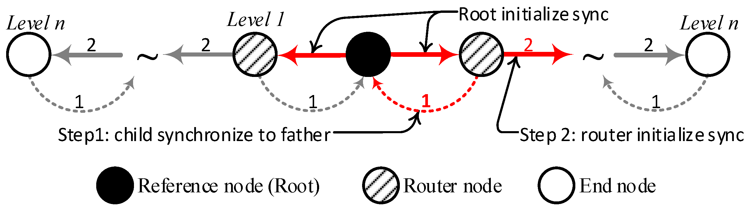
Figure 2.
Two-way time message exchange between nodes and ; there are reasonable different clock offsets caused by clock frequency, as for uplink and for downlinks.
Figure 2.
Two-way time message exchange between nodes and ; there are reasonable different clock offsets caused by clock frequency, as for uplink and for downlinks.
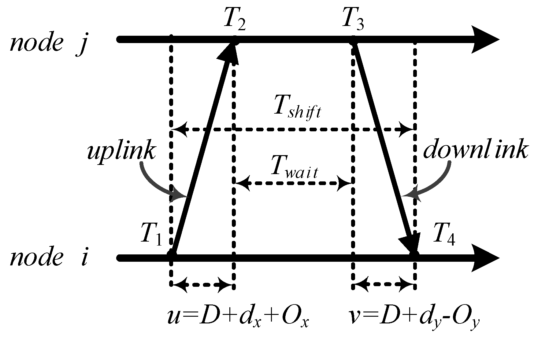
Figure 3.
The hardware clock offset and logic clock offset. Assume there is fixed clock frequency offset, the real clock offset is linear and continually increases. The logic clock offset is discrete, since the logic clock is driven by the clock granularity , the logic clock offset is the integer multiple of . The term is the cost of the clock offset increment in one , set in Equation (10), then .

Figure 4.
Multiple TTMEs . The TTME is repeated for rounds under the restriction that it should continue until . The TTME observations have a same fixed clock offset .
Figure 4.
Multiple TTMEs . The TTME is repeated for rounds under the restriction that it should continue until . The TTME observations have a same fixed clock offset .
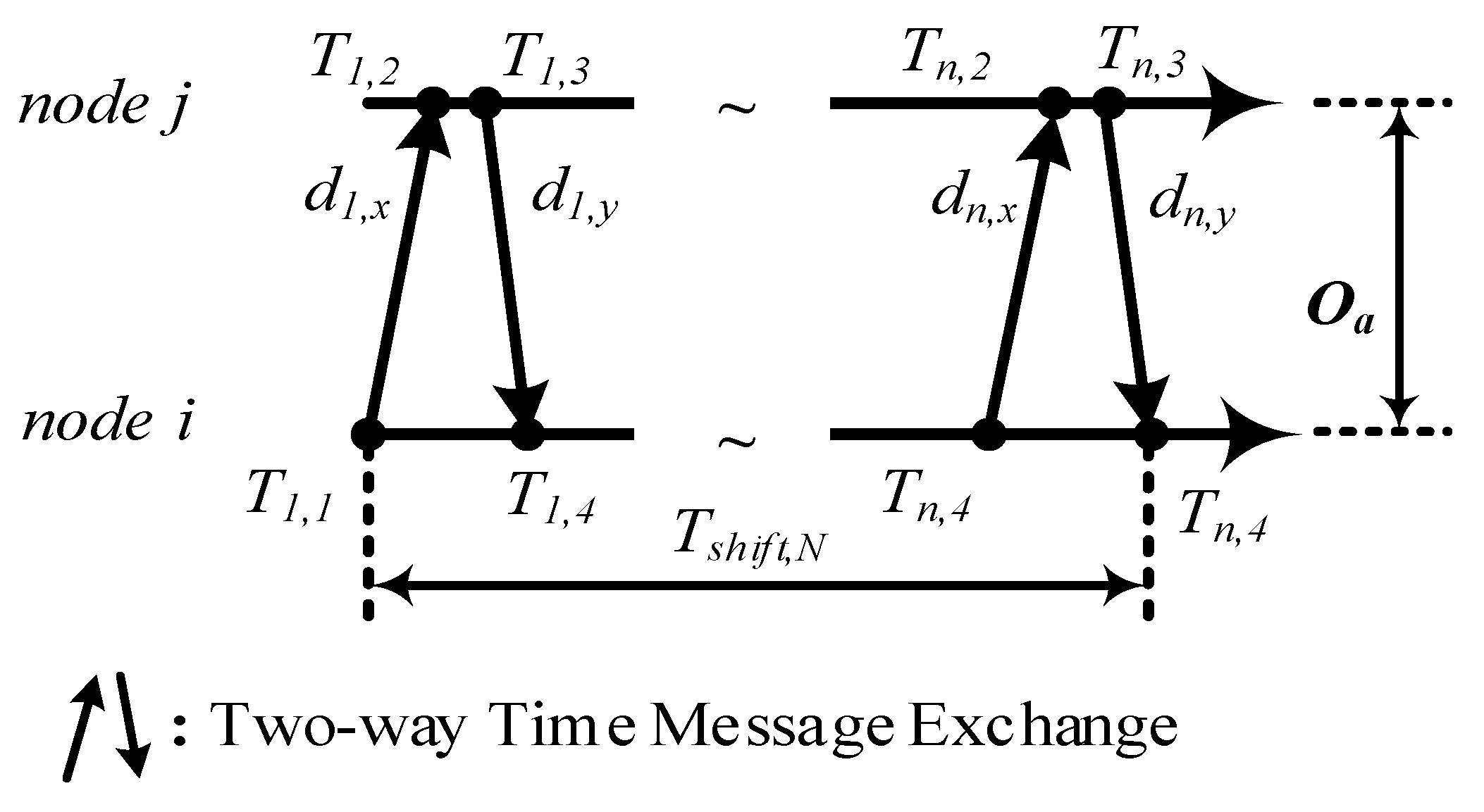
Figure 5.
CRLB and MSE of clock offset estimation, assuming the variable delay is an exponentially distributed random variable with mean .
Figure 5.
CRLB and MSE of clock offset estimation, assuming the variable delay is an exponentially distributed random variable with mean .

Figure 6.
The clock offset estimation improvement to MLE. Compared to the traditional method, the MLE estimation error is reduced fast in the first five observations and slows down after the eighth point.
Figure 6.
The clock offset estimation improvement to MLE. Compared to the traditional method, the MLE estimation error is reduced fast in the first five observations and slows down after the eighth point.
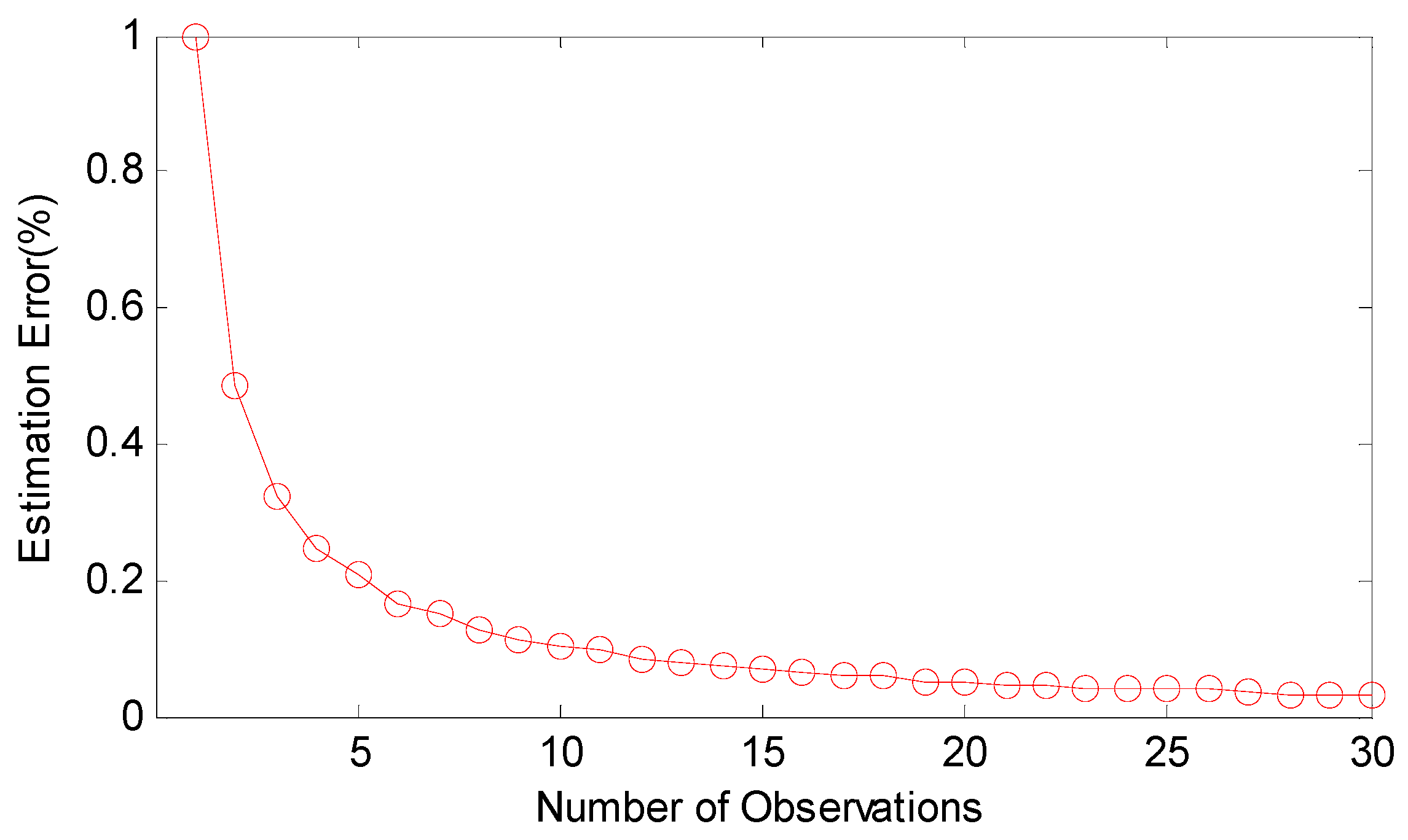
Figure 7.
The absolute synchronization error of traditional TTME.
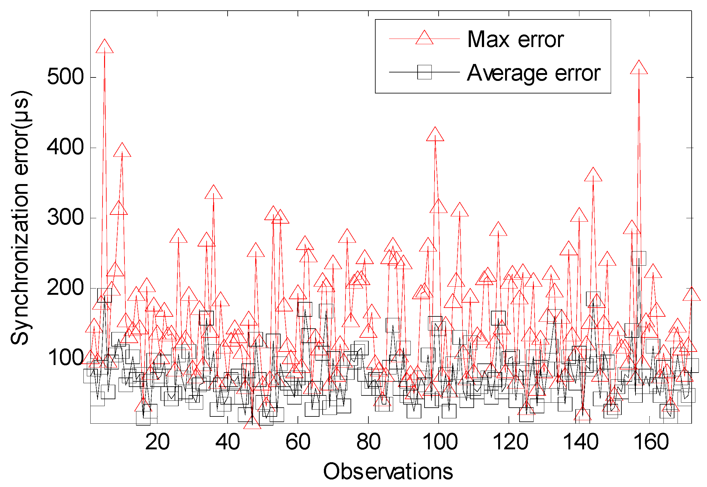
Figure 8.
The absolute synchronization error of multiple TTMEs.
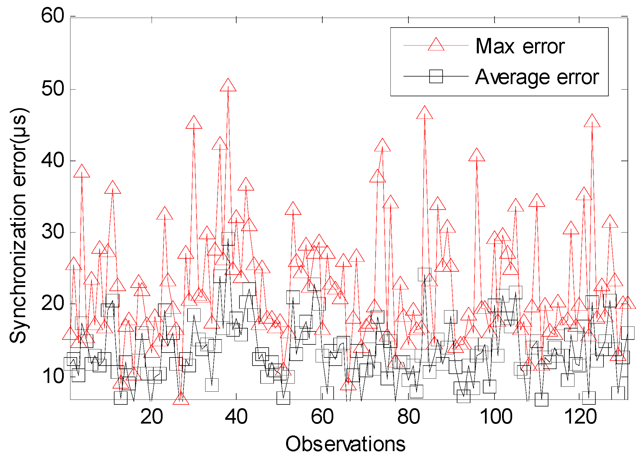
Figure 9.
The normalization MSE of the average synchronization error.
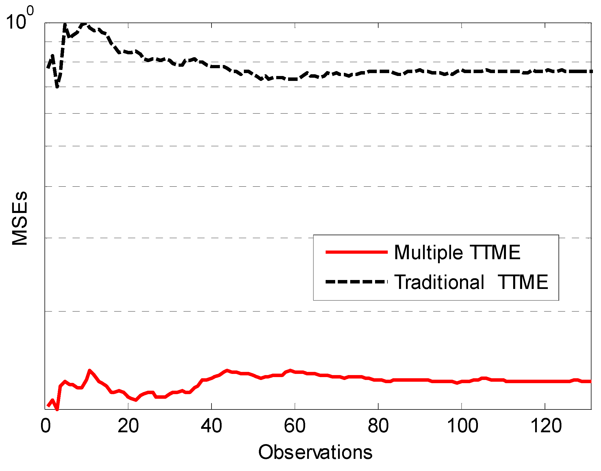
Figure 10.
Clock offset estimate precision and clock speed regress precision.
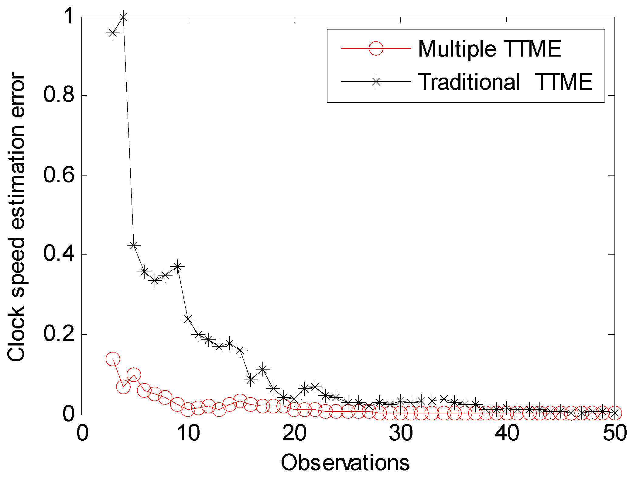
Figure 11.
The skew of traditional TTME.

Figure 12.
The skew of multiple TTMEs.


Table 1.
The synchronization error probability.
| Probability (%) | ||
|---|---|---|
| <Average Error | < | |
| Traditional TTME | 62 (75 ) | 32 (30 μs) |
| Multiple TTMEs | 51 (13 ) | 95 (30 μs) |
© 2017 by the authors. Licensee MDPI, Basel, Switzerland. This article is an open access article distributed under the terms and conditions of the Creative Commons Attribution (CC BY) license (http://creativecommons.org/licenses/by/4.0/).
Share and Cite
MDPI and ACS Style
Shi, F.; Tuo, X.; Yang, S.X.; Li, H.; Shi, R. Multiple Two-Way Time Message Exchange (TTME) Time Synchronization for Bridge Monitoring Wireless Sensor Networks. Sensors 2017, 17, 1027. https://doi.org/10.3390/s17051027
AMA Style
Shi F, Tuo X, Yang SX, Li H, Shi R. Multiple Two-Way Time Message Exchange (TTME) Time Synchronization for Bridge Monitoring Wireless Sensor Networks. Sensors. 2017; 17(5):1027. https://doi.org/10.3390/s17051027
Chicago/Turabian StyleShi, Fanrong, Xianguo Tuo, Simon X. Yang, Huailiang Li, and Rui Shi. 2017. "Multiple Two-Way Time Message Exchange (TTME) Time Synchronization for Bridge Monitoring Wireless Sensor Networks" Sensors 17, no. 5: 1027. https://doi.org/10.3390/s17051027
Note that from the first issue of 2016, this journal uses article numbers instead of page numbers. See further details here.