1. Introduction
Recently it has become evident that many processes on the Earth are closely related to the World Ocean. Besides the usual threat by ocean for navigation and activities of people in coastal areas, it strongly affects climate of the whole planet. Due to application of modern measuring equipment, the El Nino and La Nino phenomena associated with climate variations and natural calamities have been discovered. The ocean covers two third of the planet surface and is a giant accumulator of heat. Currents and sea waves determine intensity of heat and gas exchange between atmosphere and ocean. Therefore high-density measurements and reliable information on the state of the near-surface layer of the ocean is critical to draw up reliable long-term weather forecasts. Countries with predominant influence of ocean on climate have started long-period programs of ocean study, e.g., Great Britain monitors the Gulf Stream forming weather in the United Kingdom.
In the last twenty years the use of remote sensing techniques enabled one to obtain information rapidly from vast water areas. For example, the velocity and direction of wind are measured by means of scatterometers, the spectrum of large-scale roughness and internal waves by means of synthetic aperture radar, while altimeters measure the wind speed, significant wave height and the mean ocean level, from which geostrophic currents are derived.
Increasing requirements on increased global sampling and increasing reliability of the accumulated measurements has stimulated the development of a range of new remote measuring systems. Some of those are already well under way towards implementation, while others are still at the theoretical stage [
1-
6].
Nadir altimeters provide information on scattering surface along a track immediately below the satellite. Specific motion of the satellite implies that only a section of the processes occurring on the ocean surface can be captured. Since the distance between neighboring tracks may be several hundreds kilometers [
7,
8], the information proves to be rather fragmentary and insufficient for operational need.
The low repetition of observations of one and the same part of the ocean with nadir results in significant loss of information about the development/dynamics of wave processes on the ocean surface. One solution to this problem is to increase the number of satellites, as suggested, e.g., in [
9]. An alternative solution is to transfer an airborne system to a satellite platform with slight modifications [
10].
This paper presents an other approach for panoramic measurements of wind and waves using a system centred at nadir.
The basis of this analysis is the advanced theoretical scattering model which was developed during our previous researches (see, for example, [
11,
12]. In these papers we carried out the theoretical analysis and have shown that radar with knife-beam antenna pattern may be used for measurement of slopes of water surface. The experiment had confirmed the theoretical conclusion [
13,
14].
We have shown that microwave radar with knife-beam antenna may be used for retrieval of surface slopes and near surface wind speed from aircraft. The algorithm was tested from bridge and a new radar may be used for measurement of variance of slopes from aircraft.
Our radar has the simplest design in comparison with other radar systems, for example, radar with scanning beam or multi beam system. There are other radars, which are more complicated and therefore permit from aircraft to retrieve the spectrum of sea waves, for example, [
15]. However, there exist the serious problems, which don't permit to these radars make measurement from satellite. And the main reason consists in the fact that such radar require a very high spatial resolution to use the retrieval algorithm.
Our radar is able to measure only slopes and direction of wave propagation and radar may measure these parameters from a satellite. It is deals with features of radar design and with peculiarities of retrieval algorithms.
A conventional altimeter has an illuminated area with a diameter of several kilometers [
16,
17]. Using a knife-beam antenna pattern, e.g., 1° × 25°, the illuminated area at −3dB is about 14×355 km for a flight height of 800 km.
Modern numerical ocean wave models use grid cells of 50×50 km in open ocean and 25×25 km in coastal seas [
7,
18].
The resolution across the knife-beam footprint is therefore satisfactory for the study of wave processes. Temporal or Doppler selection can be used to increase the resolution in the probing (range) direction. Using a fixed knife-beam pattern aligned with the direction of flight leads to measurements of the variance of long-wave slopes, significant wave height and better near-surface wind speed. It is also possible to retrieve a friction velocity, which is more important for describing atmosphere-ocean interaction compared to the wind speed. The operation and characteristics of a nadir-pointing altimeter with a knife-beam antenna pattern aligned with the direction of motion was already considered in [
19-
21].
To obtain a wide swath (the “panoramic” mode), it is suggested to rotate the antenna about the vertical axis. As a result we have a wide swath (355 km) for a nadir-pointing antenna. Next we examine whether it is possible to get information on surface roughness in the whole swath and with what resolution. If successful, this would allow one to study not a single section of a wave process on the ocean surface as with a conventional altimeter, but a sea surface image with a high spatial resolution and the ability to capture wave dynamics and development with repeated observation from neighboring tracks or another satellite.
2. Main features of the “Panoramic” knife-beam altimeter
In what follows, numerical estimates are based assuming a flight height of 800 km, the speed of motion 8 km/s and the knife-beam antenna beam widths are 1°×25°. We suppose that an expected wavelength of radar is located from 2 up to 3 centimeters. Namely this wavelength is the more sensitive to a sea state and wind speed and may be used for remote sensing from space.
We don't analysis the features of measurements from aircraft. In this case radar will work without problems and the retrieval algorithms which were tested at the bridge may be used [
12,
13].
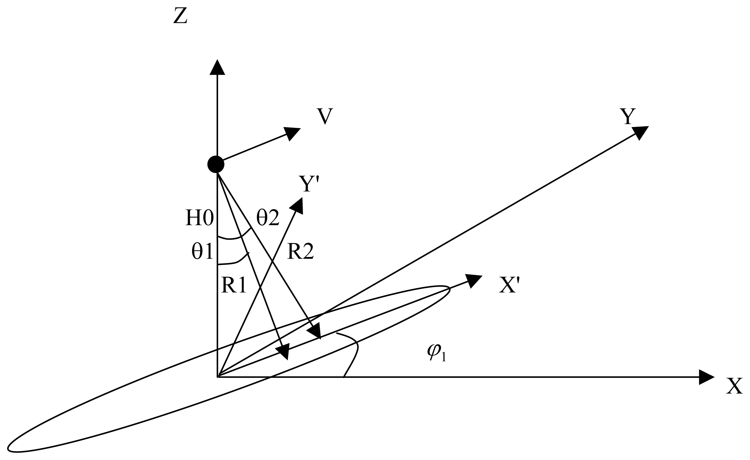
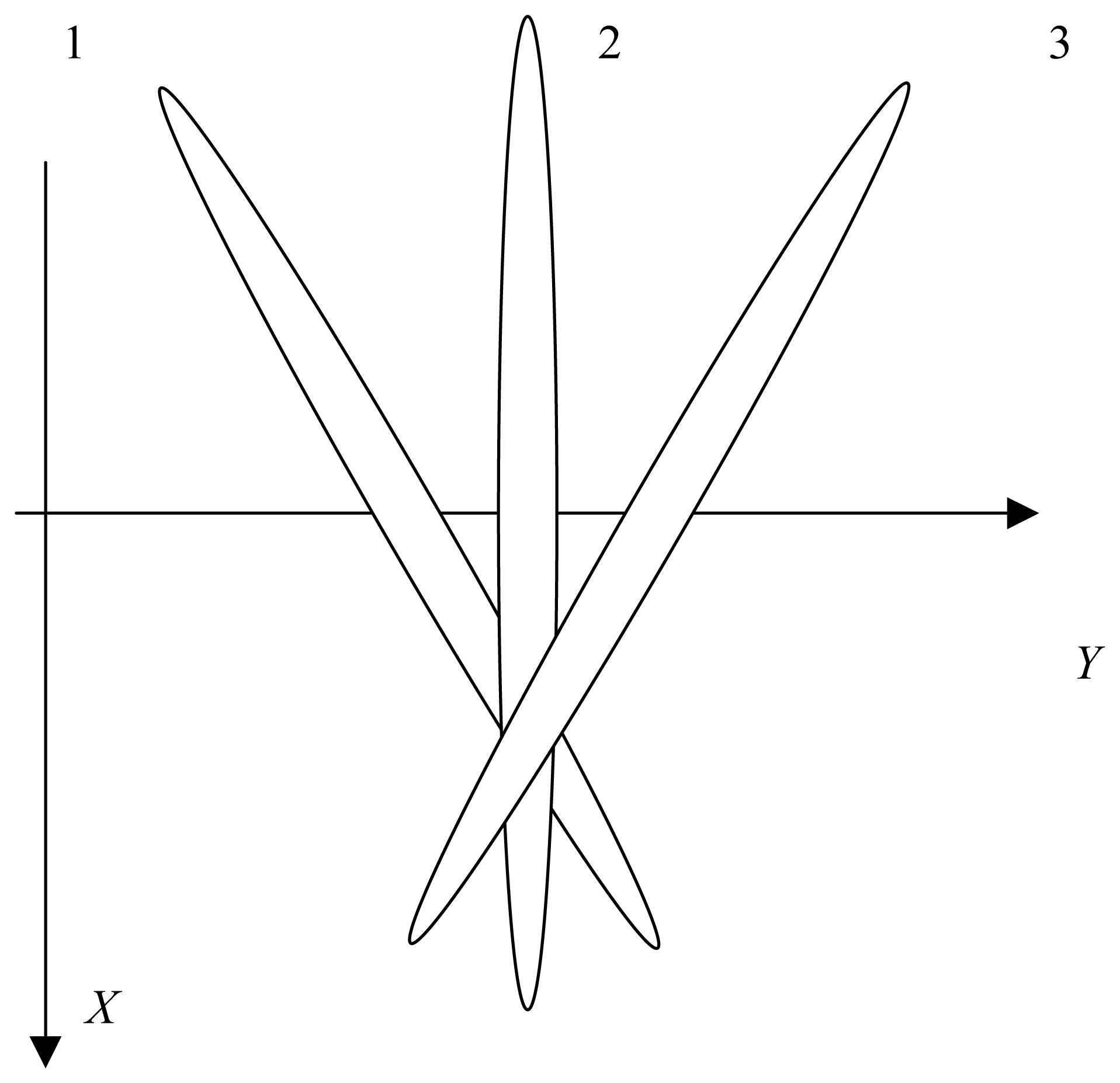
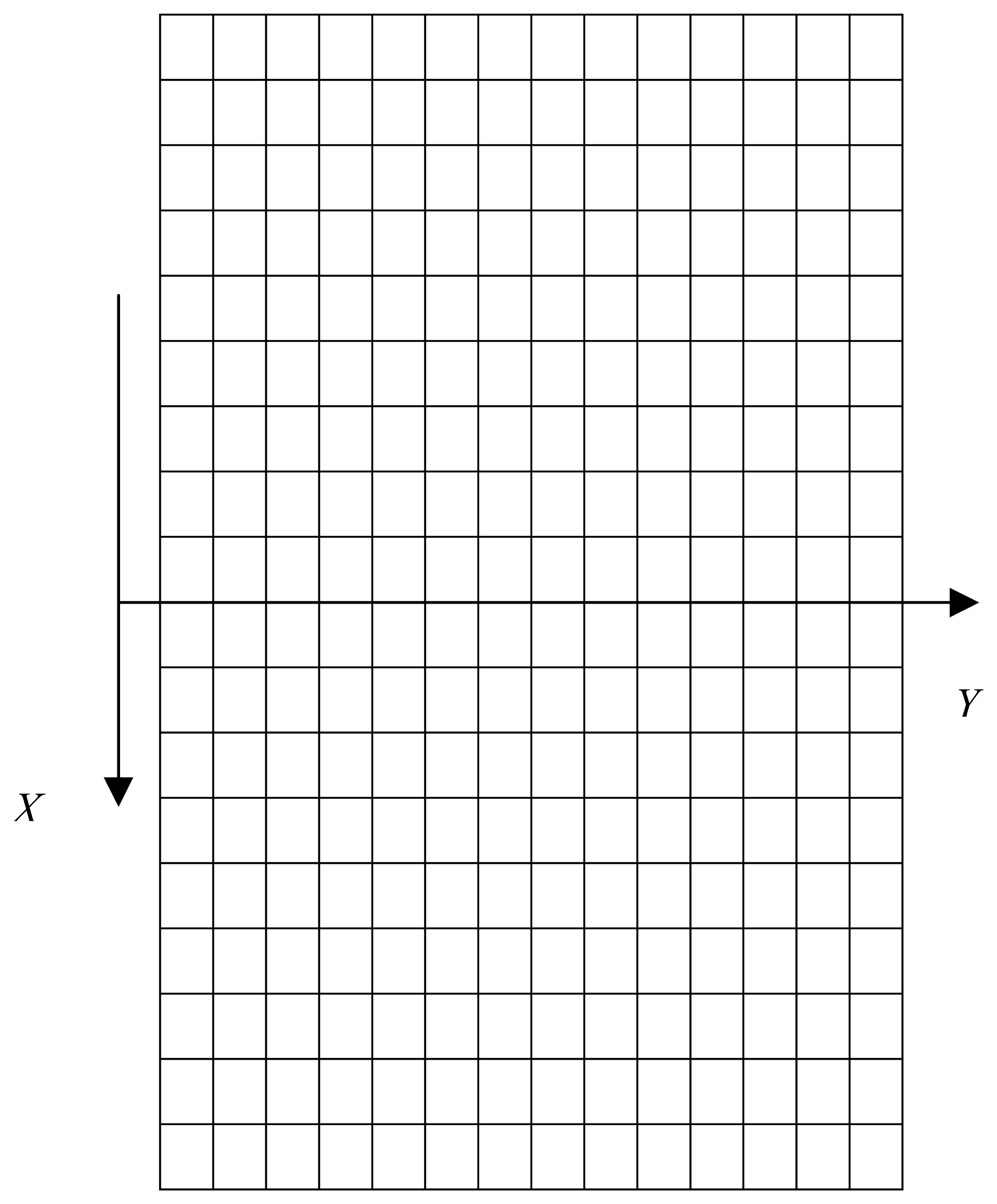
Figure 1 shows the observation scheme. Here θ
1, θ
2 and
R1,
R2 are incidence angles and slant distances for two reflecting cells on the sea surface, respectively;
H0 is the flight height. The direction of flight is chosen along the
Y axis;
V is the flight speed. We introduce the second coordinate system
X′Y′ related to the antenna: the
X′ axis is oriented along the longitudinal axis of the knife-beam footprint and the rotation angle of
X′Y′ about the first coordinate system is equal to φ
1.
We already mentioned that due to the narrow antenna beam width across the beam, an acceptable resolution of about 14 km along the Y′ axis can be achieved.
Let us now consider the peculiarities of the Panoramic mode system, i.e. when the antenna rotates about the vertical axis during the motion. The first difference compared to the case where the knife-beam antenna is fixed is that radar cannot continuously see all elementary cells (
Fig. 2). How often an elementary cell is observed depends on the rotation speed of the antenna.
If the antenna footprint is oriented along the direction of flight, an each elementary cell is observed at all incidence angles within the antenna pattern, thus the processing procedure developed in [
19-
21] can be employed for the retrieval of slope variance in each cell. This approach is not applicable in the rotating antenna case, since each elementary cell is visible only at a few incidence/azimuth angles.
Thus a new algorithm needs to be developed to determine slope variance in the panoramic mode to take into account the specific nature of the measurement scheme.
As is known, at small incidence angles, backscattering is dominated by quasi-specular reflections from wave facets oriented perpendicularly to the incident radiation field. In the general case, the backscattering radar cross section is represented by the formula [
22–
24]:
where
and
are the variances of the slopess of large-scale waves along the
X′ and
Y′ axes, respectively. Here we neglect the correlation coefficient between slopes of two mutually perpendicular directions;
U10 is the wind speed at 10 m height; θ
1 is the incidence angle.
This formula was obtained in the assumption of Gaussian surface for large-scale waves (Gaussian function of heights). A lot of experiments confirmed this assumption for large-scale waves. The small-scale waves may possess by other distribution.
The effective reflection coefficient
Reff is introduced instead of the Fresnel coefficient [
22-
24]. This coefficient takes into account the attenuation of the reflected field due to small ripples on the surface. The spectral density of ripples depends on the local wind
U10, to be more precise on the friction velocity
u*[
25,
26]. Though great attention has been paid to the problem of specifying the correlation between the wind speed at 10 m height and the friction velocity, e.g., [
27–
29], the problem on the correct conversion from
U10 to
u* is not solved yet. The velocity profile in the boundary layer depends on atmospheric stability and parameters related to large-scale waves.
We suppose that new microwave radar will have a short wavelength, for example, 2-3 cm. In according with two-scale model, the wave spectrum may be divided into two parts: large-scale waves and small-scale waves. The small-scale waves are sensitive to wind speed. The large-scale waves depends not only wind speed but from swell and stage of development of wind waves. In according with two-scale model exist the limit (k
b) between two parts of spectrum [
22-
24], for example, waves which longer 0.5m are large-scale waves and waves which shorter 0.5m are small-scale waves for radar wavelength is equal 3 cm. Also there exist the dependence of limit (k
b) from wind speed. However, we will use the integral characteristic (variance of slopes) and some fluctuation of limit is not important for result.
From
Eq. (1), we see that the backscattering radar cross section depends on slope variance of large-scale waves. In the case of fully developed wind waves, the wave spectrum and all surface parameters are determined by the wind speed. As a result, the relation between the backscattering radar cross section and wind speed becomes unambiguous, and hence the wind speed can be retrieved accurately by means of the backscattering radar cross section.
However, the most frequently occurring state on the ocean surface is mixed sea. In this case, swell unrelated to the local wind speed, changes the large-scale roughness parameters. As a result, the relationship between the backscattering radar cross section and wind speed becomes ambiguous [
30]. Swell most strongly affects surface roughness characteristics at low wind speeds (< 6 m/s) [
31]. Since no information on the variance of long wave slopes is available from standard radar measurements, this ambiguity cannot be eliminated and causes sea state related errors when retrieving wind speed from the backscattering radar cross section [
32-
34].
3. Retrieval of long wave slope variance
As already mentioned above the radar with knife-beam antenna pattern may measure the variance of surface slopes from aircraft [
12-
14]. If radar will be installed at the satellite the footprint will be large (a few hundred kilometers) and a radar will measure only some averaged variance of slopes. Hence it is necessary to develop the new retrieval algorithm.
The following method is suggested to measure slope variance in a wide swath with high resolution.
When a knife-beam antenna (1°×25°) is rotating, a wide swath is illuminated, which can be split into elementary scattering cells employing temporal or Doppler selection.
Two sequential cells along the
X′ axis will differ in incidence angles. For small cells, e.g., 14×14 km one can neglect variation of roughness parameters either inside a cell or between neighboring cells. To retrieve the slope variance along the probing direction we use the formula derived from
(1):
where θ
1 and θ
2 are the incidence angles of two elementary cells, while σ
0(θ
1) and
σ0(
θ2) are the radar cross sections of these cells, respectively.
In our previous investigation we have shown the advantage of knife-beam antenna in comparison with conventional radars, for example, [
19,
20].
If we want to use our radar from satellite we meet problem of large size of footprint. The size of footprint is bigger than scale of some wave process on sea surface. Therefore the division of the footprint into a few scattering cells is solution of this problem.
There are other radar systems which permit to work with small cells from space, for example radar with scanning beam or multi-incidence radar system.
The advantage of our radar consist in more simple construction in comparison with other radars: knife-beam antenna which rotated around vertical axis and conventional microwave transmitter. Antenna is more compact in comparison with other antenna systems. The characteristics of radiated impulse are identical for all scattering cells. The new system is a flexible system. Radar may possess the different spatial resolution that depends from data processing.
The certain shortcoming of the new radar is a power budget. However it is a solved problem because the required power will be significantly less than for conventional scatterometer or radar system suggested in [
5]. These radars have worked at middle incidence angles where the reflected power significantly less than at nadir probing.
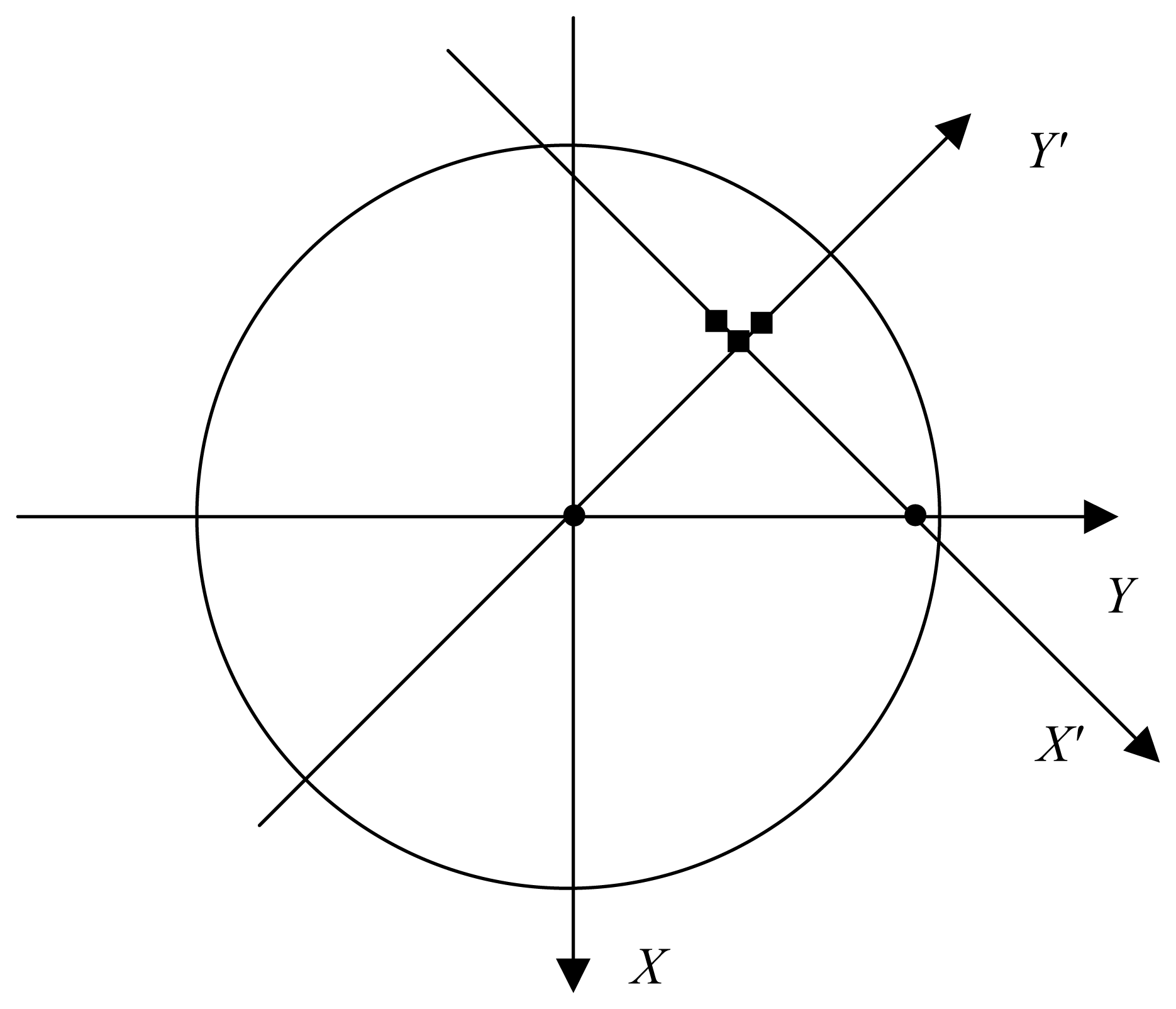
It is known that the total slope variance is the sum of slope variances measured in two mutually perpendicular directions. Thus to find out the total slope variance of the surface in each elementary cell, one should measure slope variance in this cell at various azimuth angles using antenna rotation during radar motion (
Fig. 3).
The squares in
figure 3 are a representation of two neighboring cells. The index “
x1” in formula
(2) means that slopes are retrieved along the
X′ axis.
As a result we find that if the second measurement is made at an azimuth angle of 90 degrees with respect to the first one, it is possible to determine the total slope variance
in the elementary cell, i.e. here
refers to the second measurement of
when the X′ axis has rotated by 90 degrees:
.
If measurements are performed at different azimuth angle (≠ 90°), one can – assuming one knows the character of the azimuth dependence of slope variance – know the slope variance in any direction and calculate the total slope variance. Hence, the algorithm is similar to that used determine wind direction by means of scatterometer data. But now this provides an opportunity to measure the direction of propagation of large-scale waves.
While Synthetic Aperture Radars (SAR) provide images of swell waves from which direction of propagation can be derived, the image synthesis of SARs introduces a high frequency cut-off which means only waves longer than 100-120 m can be detected [
18]. There are also concerns about the accuracy of SAR's wave direction whenever the wave field includes azimuth traveling waves. In the case of the panoramic knife-beam altimeter, there are no such wavelength or wave direction limitations.
In addition due to wave profile asymmetry, the direction of wave propagation with our method can be determined unambiguously.
The dependence of the backscattering radar cross section on incidence angle was investigated during an experiment carried out on a bridge over the Oka river [
13,
14]. The same dependence will be obtained after splitting the antenna footprint into elementary scattering cells. Measurements have shown that there is a difference between the slope variance on the front and the rear of long waves: the front slope variance was 0.0142, while that of the rear one amounted to 0.0114. Hence it is seen that the difference between front and rear wave slopes is measurable by the suggested method and this permits to unambiguously determine the direction of wave propagation.
Just now we can not be sure that this difference will be clear selected for all sea conditions. We have not enough experimental data. The future experiment will permit to check this hypothesis in detail. Therefore we can not promise before experiments the removal the uncertainty in azimuth, so called the problem of 180 degrees.
When splitting the illuminated footprint into elementary scattering cells, we encounter an influence of the antenna pattern. Though the antenna beamwidth chosen rather wide (e.g., 25 degrees), it still affects slope variance retrieval. The fact is that as the incidence angle increases the antenna pattern reduces the reflected signal power. After splitting into elementary cells, one should make power correction and only then apply formula
(2). Let us consider this in detail.
The antenna pattern is assumed to be Gaussian and can be represented by the expression:
where
δx and
δy are the beam widths at the half power level along
X′ and
Y′ axises correspontly.
To apply the correction, one should multiply the backscatter coefficient in an elementary cell by the correction factor related to the effect of the antenna pattern. To take this into account we must compensate the decreasing of reflected power due to antenna pattern (see formula
(3)). The conversion formula is:
where sin
θ =
x/
R0.
A different more rigorous method to determine slope variance is based on the use of the Doppler spectrum model developed for a radar with a knife-beam antenna pattern [
11]. In this case the reflected power for each elementary cell does not need to be corrected for the effect of the antenna pattern; the slope variance is calculated from the difference of the reflected signal power between neighboring cells. Here we do not use the absolute value of reflected power.
To calculate the backscatter coefficient of an elementary cell i, one should integrate the Doppler spectrum
Sd(
ω)as follows:
where the frequency integration limits (
ωi−1÷
ωi) determine the cell position and size. The backscatter in the neighboring cell i+1 thus amounts to:
and thus the difference is found out easily as:
For a moving platform, the variation in the reflected backscatter between cells selected by Doppler is mainly dependent on slope variance. The general formula for the Doppler spectrum is rather cumbersome, so we present here as an illustration a simplified expression for the Doppler spectrum when the antenna pattern is oriented along the flight direction:
where
k is the wavelenght of radar.
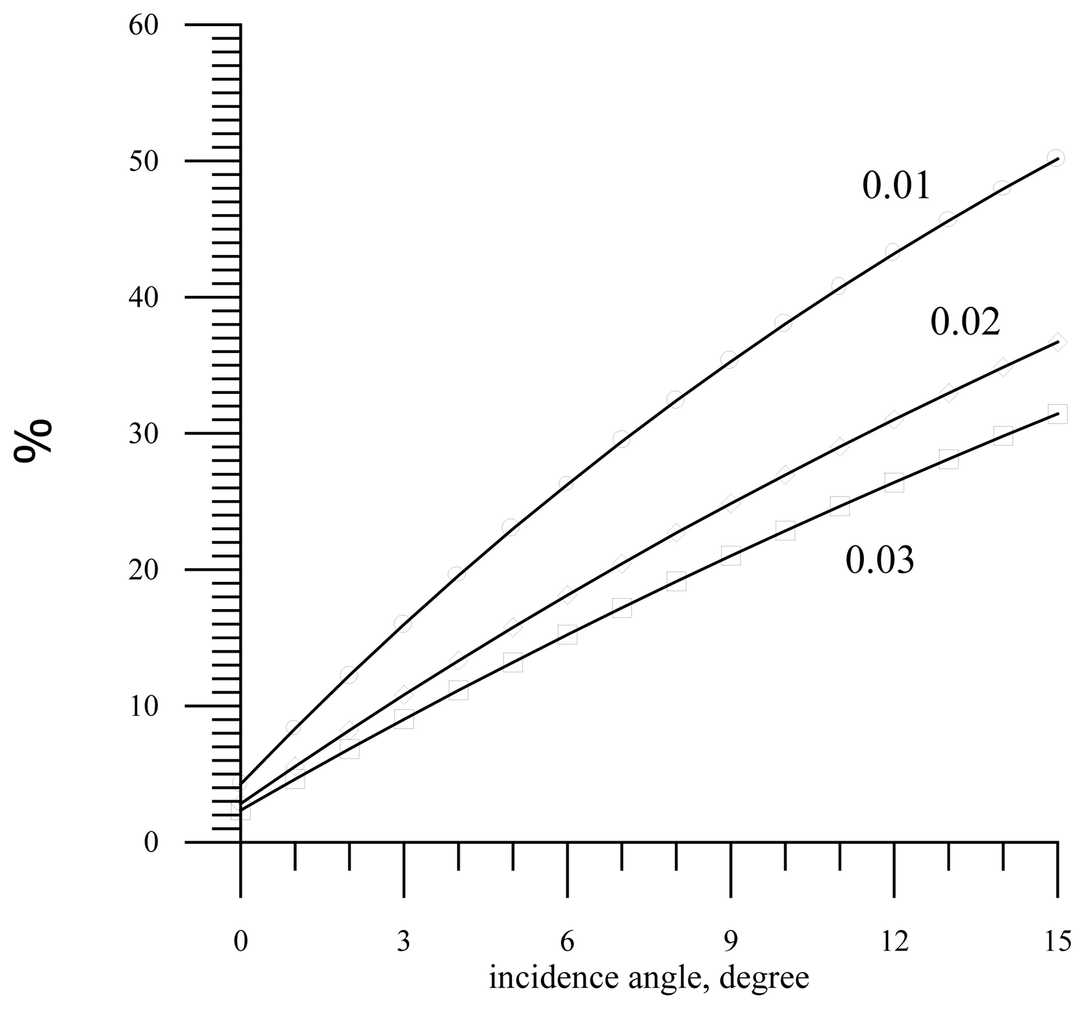
The simplest way to illustrate this method is to construct the nomograms for various values of the slope variance. The value of Δσ
0(θ
i, θ
i+1)/ σ
0(θ
i) (in per cent) is plotted against incidence angle in
Fig. 4. It is seen in the figure that for incidence angles over 3-4 degrees, the backscatter difference becomes measurable and can be used for slope variance retrieval.
A simple way to measure slope variance would be to compare the measured backscatter difference with the values of the theoretical model depicted by the nomogram. An important advantage of this method is that it depends not on the absolute value of the power (which is affected by numerous factors), but depends on the difference in reflected backscatter at two incidence angles, which depends only on slope variance.
4. Selection of the spatial resolution in range
The azimuth resolution is determined by the antenna beam width across the beam. As we have seen before, if the antenna pattern width is assumed to be 10 at the half-power level (-3 db), the cell resolution in azimuth on the surface is ∼ 14 km. This value depends on incidence angle and flight height.
The range resolution along the probing direction can be chosen within wide limits depending on the processes to be observed, and can vary from tens of meters to tens of kilometers. The range resolution can be achieved either with temporal or Doppler selection.
If necessary, temporal selection permits to obtain resolution of the order of several tens of meters, but this imposes stringent technical requirements on the radar parameters, in particular in terms of pulse duration and emitted power.
Range resolution obtained with Doppler selection is characterized by relatively uniform distance increments and less stringent technical requirements for the radar. In fact, the transmitter can even operate in continuous wave (CW) mode. Doppler selection introduces a dependence of the resolution on the angle between the direction of motion and the probing direction: the resolution in range worsens when this angle φ1 is small.
The Doppler selection is based on the Doppler shift of reflected signal. This idea is used in conventional scatterometer. Let us estimate the azimuthal limitation of Doppler selection. If we suppose that may separate cells which differ on 20m/s, we have the following limitation for angle φ1: selection procedure can not be applied in sector from -8° to 8°. In result we may lose one measurement for some cells and radar will see these cells only 5 times instead of 6 times.
In contrast to what is the case with temporal selection, the size of the scattering area obtained with Doppler selection depends only weakly on incidence angle, which makes it more convenient from the viewpoint of further processing.
The second factor influencing the choice of range resolution is the dependence of the backscattering radar cross section on incidence angle. It is evident that formula
(2) can only be employed, if there is a measurable difference between the backscattering radar cross sections for two neighbouring cells. It is known from experiments that if the incidence angle varies from 0 to 10 degrees, the backscattering radar cross section changes by 5-10 dB depending on the wind speed [
22-
24]: the higher the wind speed, the smaller the difference in radar cross section.
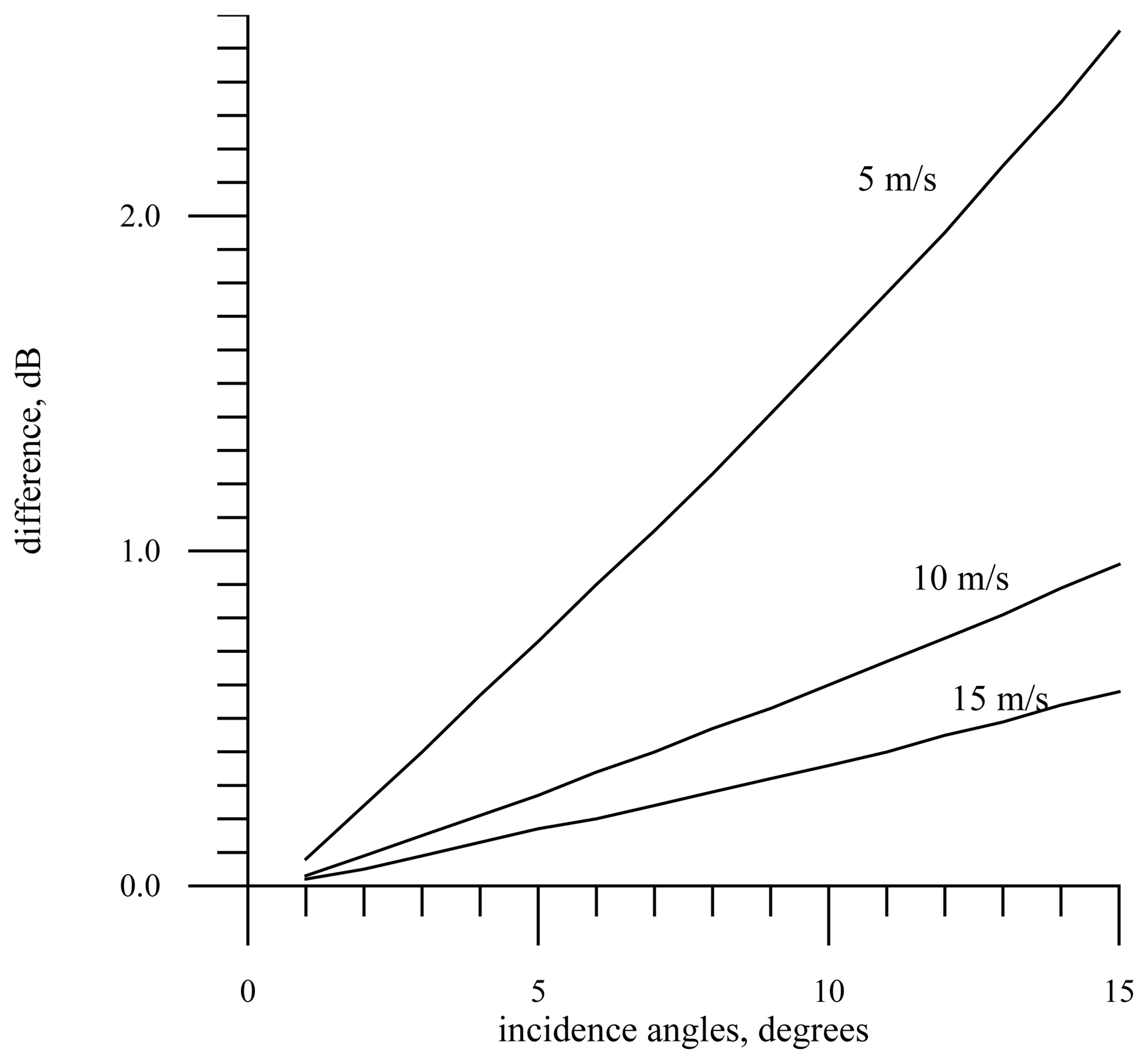
On the basis of these results, we have constructed in
Figure 5 the dependence on incidence angle of the backscattering radar cross section difference Δσ
0 = σ
0(θ
0) − σ
0(θ
0+1) across two neighbouring cells separated by 1 degree. Assuming typical measuring equipment sensitivity and taking into account reflected signal fluctuations, the difference should be more than 0.1–0.2 dB to be detectable [
11,
12].
Therefore,
Figure 5 shows that it will be possible to measure slope variance̵s outside a circle of radius of 3-4 degrees from nadir at any wind speed, and at low wind speeds within this circle too. However, at a high wind speed slope variance inside the circle would be retrieved with a significant error.
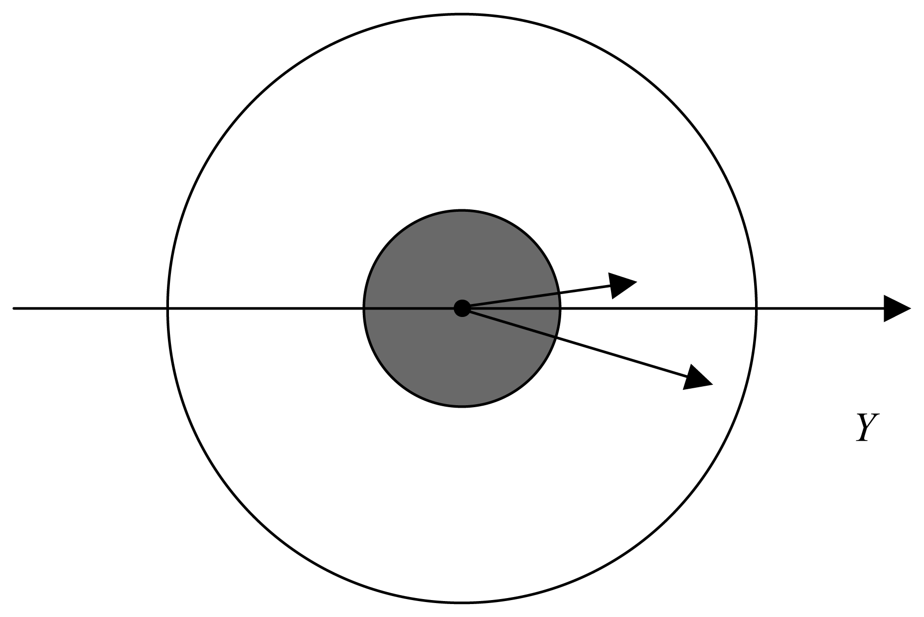
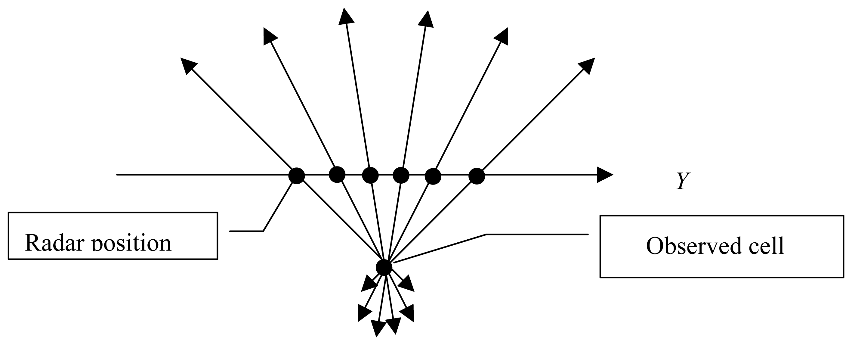
Nevertheless, due to the antenna rotation and the motion of the satellite it is easy to measure the slope variance in a given cell located in the footprint directly under a satellite (in a “dark” circle) when viewed at a different time from another incidence angle̵s (
Fig. 6). Besides, it is possible to increase the difference in backscattering radar cross sections by using not neighboring cells, but every other one. As a result, the difference of incidence angles between cells will be 2 degrees, though the equivalent spatial resolution would still remain better than 50 km.
We may use the special synthesis procedure which was developed in [
20,
21]. Due to antenna rotation the radar will see the cells along track of radar. During flight due to movement the radar will see the selected cell under a few incidence angles. Collecting all the data about this cell (different incidence angles/different times) we may used developed retrieval algorithm [
20,
21] to retrieve the variance of slopes. It is permits us to measure the variance of slopes by other algorithm and additional control of new algorithm may be organized.
5. Determination of direction of large-scale wave propagation and wind speed
The next step is to determine the direction of large-scale wave propagation in each elementary scattering cell. For this purpose one should measure the surface slope variance in each cell at various azimuth angles and plot the azimuth dependence of slope variance. The maximal value of slope variance shows the wave propagation direction. The algorithm uses the peculiarities of the azimuth dependence of slope variance and thus is analogous to the algorithm used for retrieving wind direction from scatterometer data.
For example, one may utilize the solution of the following set of equations. The relation of slope variances at an arbitrary observation angle
ϕ0 from the direction of wave propagation can be represented by [
35]:
where
and
are the slope variances along and across the wave propagation direction, and
ϕ0 is the angle between the probing direction and the wave propagation direction. We must carry out measurements for each scattering cell under at least 3 different azimuth angles in order to solve this set of three equations with three unknowns
,
,
ϕ0).
If the angle between two measurements belonging to one cell is not equal to 90
0, i.e. φ
2− φ
1 = Δφ≠90
0 the equation will be more complicated. For example, the second equation becomes:
If mixed sea (wind waves and swell) is present on the surface, the set contains six unknowns and six equations are required for solution [
35]. In this way one can retrieve not only the propagation direction of wind waves, but also direction of swell and their variance of slopes. Measurements at six azimuth angles should be performed for each cell.
The new radar measures the total variance of slopes in every cell which is sum of slopes both wind waves and swell. Is known that swell strong affects on SWH, especially at low wind speeds. We know that the main contribution to variance of large-scale waves gives the average sea waves from a few tens meters to the right limit kb of large-scale waves. Therefore the contribution of swell to variance of slopes is small. And we think that in the most cases the radar will see the direction of propagation of wind waves and can not separate the direction of swell. But in theory the possibility of determination of direction of swell propagation exist. Only experiment will permit to check the suggested algorithm and gives the answer on this question.
The radar sees each cell at different azimuth and incidence angles due to the platform motion and antenna rotation. We demand that the minimal azimuth angle in the observed band between two measurements of one and the same cell be not less than 90 degrees. On the one hand, this demand decreases the width of area where surface parameters may be retrieved, and on the other hand it permits to minimize an error of slope variance retrieval and determine the wave propagation direction more exactly.
With allowance for this requirement the width of swath decreases from 355 km to 250 km. Information is naturally gathered in the whole swath, the slope variance and other characteristics can be retrieved everywhere. One should only bear in mind that outside the limits of 250 km area, the error in determining total slope variance and direction of wave propagation increases.
Let the radar see each elementary cell 6 times, i.e. at six azimuth angles. Three antenna rotations are sufficient for that purpose, since a scattering cell is observed 2 times per rotation. The width of swath satisfying these conditions is about 250 km.
Figure 7 shows the antenna positions when observing a chosen cell during the flight time, i.e. at the speed of 8 km/s a satellite sees the cell for about 31 s. Hence the rotation speed needs to be less than 6 rotations per minute.
As a result we measure slope variance in each cell at six azimuth angles, then determine the total variance and the direction of propagation of large-scale waves in each elementary scattering cell. Outside the 250 km swath the error increases rapidly, but if necessary one can analyze data in the whole swath.
After determination of the variance of slopes and direction of wave propagation we may attempt to retrieve the wind speed.
Exist two ways which will be tested in future. The first way is a classical approach. This way is used always for scatterometer and altimeter and is based on regression analysis of experimental data. We carry out experiment to measure the dependence of radar cross section from wind speed. The regression analysis is used to find a equation for retrieval algorithm.
The second way will use the measured by our radar the variance of slopes. Here the experimental data also will be used but we will develop a two-parameter retrieval algorithm taking into account the variance of slopes too. Theoretical considerations show that precision of retrieval algorithm will be better.
The wind speed retrieval algorithm will be developed after the experiment.
6. Increase of spatial resolution in azimuth
We have considered above the mechanisms of spatial resolution selection by means of the antenna pattern in azimuth and temporal/Doppler selection in range. It has been shown that it is easy to obtain high range resolution but more difficult to improve azimuth resolution.
Azimuth resolution is defined by the antenna beam width across the beam. In order to maintain nadir within the antenna beam in spite of platform attitude fluctuations during a flight, the antenna beam width should be at least 1 degree [
16,
17]. This condition limits the opportunity of improving the resolution in azimuth by decreasing the width of the antenna pattern.
However, our research has shown that azimuth resolution can nevertheless be improved by applying a special processing technique.
Let us assume in the first instance that temporal selection is used to form elementary scattering cells of size, e.g., 14×1 km.
The surface area sampled by one cell during one rotation of the antenna corresponds to ring 1 km wide (where the distance in range between the outer and inner circles is determined by the range sampling time τ). The arc length of the cell depends on the antenna beam width, i.e. in the considered case it is approximately equal to 14 km.
In the general case the Doppler shift value
Vdop is given by the formula:
where θ
1 is the incidence angle, φ
1 is the probing direction (see
Figure 1).
Using temporal sampling to define an elementary cell within the footprint means the incidence angle is fixed and the Doppler shift for this incidence angle can be known.
In this case changes in Doppler shift within the cell can be related to changes in azimuth angle within the elementary cell (here by 1 degree) by:
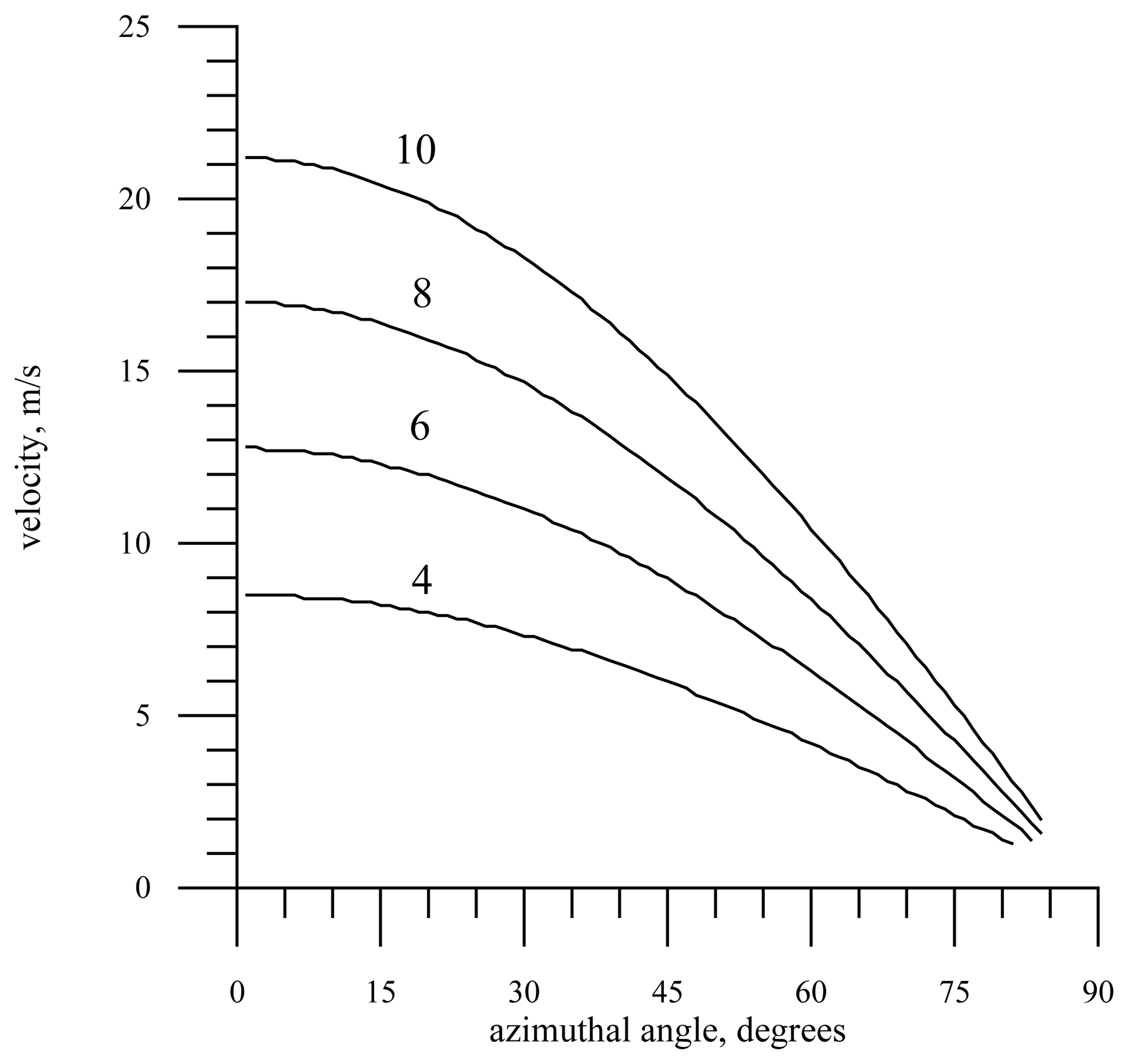
The change in Doppler shift for a 1 degree azimuth increment within one elementary cell is shown in
Fig.8 against azimuth angle for several incidence angles. Thus we see that the change in Doppler shift with azimuth inside the cell can be used to subdivide this cell into several parts. If we assume the system can detect Doppler shift changes equivalent to Δ
V =5 m/s, we find that the elementary cell can be subdivided into 2-4 parts in azimuth and thus lead to increased resolution in azimuth of order 4–7 km.
In this case is required the use of the temporal selection at the first stage to select the cell for further improvement of resolution taking into account the Doppler spectrum.
7. Data post-processing
Here we define a possible data post-processing procedure for the panoramic mode of radar.
When the radar moves along the Y axis, a swath of the width 355 km is illuminated. Taking into account the restrictions we have imposed on the azimuth observation angles (see section 5), the width of the usable swath reduces to 250 km.
Assuming that the incidence angle step is 1 degree, we now split the backscatter measurements over the 250 km wath into a rectilinear grid of cells of size, e.g., 14×14 km (
Fig.9).
Using the algorithms defined in earlier sections, we retrieve slope variance, wind speed and wave direction of propagation in each cell. This coarse resolution grid gives a general overview of surface processes.
This approach provides a two-dimensional map of the scattering surface. It makes it possible to visualize a slope field and a wind speed field depending on the problem to be solved.
Applying Doppler/temporal selection it is now easy to improve distance resolution, e.g., to form cells of the size 14×1 km and investigate finer surface processes. In this case it might be useful to employ an average value of slope variance calculated in a larger cell to reduce the fluctuations and enable improved retrieval of the wind field structure.
For a detailed study of a given surface process, one can increase the spatial resolution by combining temporal and Doppler sampling. In this case the elementary cell size can reduce to as little as 5×0.5 km (see section 5). Given that the achievable precision for the retrieval of slope variance, wave direction of propagation and wind speed is driven by fluctuations of the reflected signal power, the suggested post-processing would return better results than those obtained from applying the available algorithms to direct measurements.
8. Significant wave height retrieval in a wide swath
Significant wave height is a useful parameter to describe wave processes on the ocean surface. Here we have discussed the basic ideas which may be used at the development of the new radar system measuring the SWH in a wide swath. We don't analyse the characterics of future radar but only discuss the basic ideas of his working and measuring.
Conventional nadir altimeters provide the possibility to measure significant wave height along the track by measuring the time it takes for the reflected pulse to reach its maximum value (i.e. the duration of the leading edge of the altimeter waveform). However, there are no techniques at present to measure significant wave height in a wide swath.
The presence of crests and troughs on the real sea surface increases the duration of the reflected pulse leading edge because of the increased path difference introduced by the presence of the waves. Significant wave height is measured by measuring the slope of the leading edge at the mid point of the waveform [
15,
16]. Comparison of altimeter significant wave height with buoys measurements has shown high accuracy of the algorithm with errors not exceeding 10% or 0.5m (whichever is largest).
The main requirement for measuring significant wave height is the need for reference point indicating the start of the reflected signal leading edge. In a pulse-limited nadir viewing case, the incidence angle inside the illuminated footprint does not change, thus it is possible to measure precisely when the reflected power reaches its maximum value and from this deduce the duration of the leading edge, its slope and hence significant wave height.
However the problem of determining significant wave height in each cell of a wide swath cannot be solved in such a way.
If measurements are carried out away from nadir using an altimeter with a narrow antenna pattern, it is more difficult to measure the mean mean sea level. At the same time the measurement accuracy of significant wave height does not worsen away from nadir.
The fact is that at off-nadir incidences, the significant wave height still affects the duration of the reflected pulse's leading edge. Hence, one could use a radar with a narrow antenna pattern, e.g., 0,5°×0,5°, and apply a scanning mode, say over 14° on either side of nadir, and measure the significant wave height with this technique over a wide swath with necessary resolution.
But this approach imposes serious technical requirements on the measuring system, thus we suggest a different method. Let us first consider how one can achieve a narrow antenna pattern and whether it is possible to find out the wave height with it.
First of all, a narrow antenna pattern can be used to single out a precise area of interest and the reflected signal has information precisely on this part of the surface. The incident pulse hits the surface and is reflected from it. Thus an initial reference point appears when the leading edge of the pulse touches the wave crests and the received power starts to increase. A final point corresponds to the rear edge of the incident pulse reaching the troughs. The slope of the reflected pulse leading edge can be measured in this way for the cell isolated by the narrow antenna pattern. If scanning the beam in incidence the wide swath is split into elementary cells and the wave height can be determined in each cell.
When measuring with a wide antenna beam, there is only one reference point which corresponds to the incident pulse hitting the surface directly under the radar (at nadir). Hence a new approach needs to be developed for measuring the slope of the “leading edge” of the reflected pulse for cells in a wide swath.
To measure significant wave height in a wide swath, it is necessary to define a reference point for each elementary cell. The reference point is a time when the emitted electromagnetic wave begin to return from selected cell. If we have, for example, ten cells we must have 10 reference points. To solve this problem we suppose an using the Doppler frequency shift of the reflected signal. In this special case radar will work in impulse mode with Doppler selection.
The temporal selection may be used too but in this way we meet some problems, for example, exist two cells at identical distance and we must use Doppler shift to separate these cells. Therefore, in this case the Doppler selection for retrieval algorithm is preferable.
As is well known, for a constant platform velocity and a given antenna rotation angle, the measured Doppler shift depends on the incidence angle (see
Eq. 5). It is possible to set, at the input of the receiving device, specific frequency filters with rectangular amplitude-frequency characteristics tuned to select specific elementary cells. Thus, by focusing on the received power in this filter, we can measure the rise and fall in received power in each elementary cell.
Plots of the received power are shown in
Fig.10 for the frequency filter with transmission bands 500-510m/s and 510-520m/s (the pulse duration is 100 ns, the wind speed is 10 m/s. As is seen from the figure, increasing Doppler velocity (i.e. incidence angle) decreases the reflected signal power and shifts the pulse along the time axis.
If the surface is immobile, the significant wave height can be easily determined from the slope of the leading edge of the reflected signal as with conventional altimeters. In this case, reflections from wave crests correspond to the start of the leading edge of the reflected signal. When the incident signal reaches the wave troughs, the received power becomes constant (assuming the correct choice of pulse duration) because the size of the reflected area is defined by the bandwidth of the frequency filter and does not change.
To reduce the influence of using off-nadir incidence angles, one can sum up the pulses belonging to one cell when measured at different azimuth angles. Numerical estimates of the wave height could be obtained more precisely by measuring the leading edge of the received pulse formed in such a way.
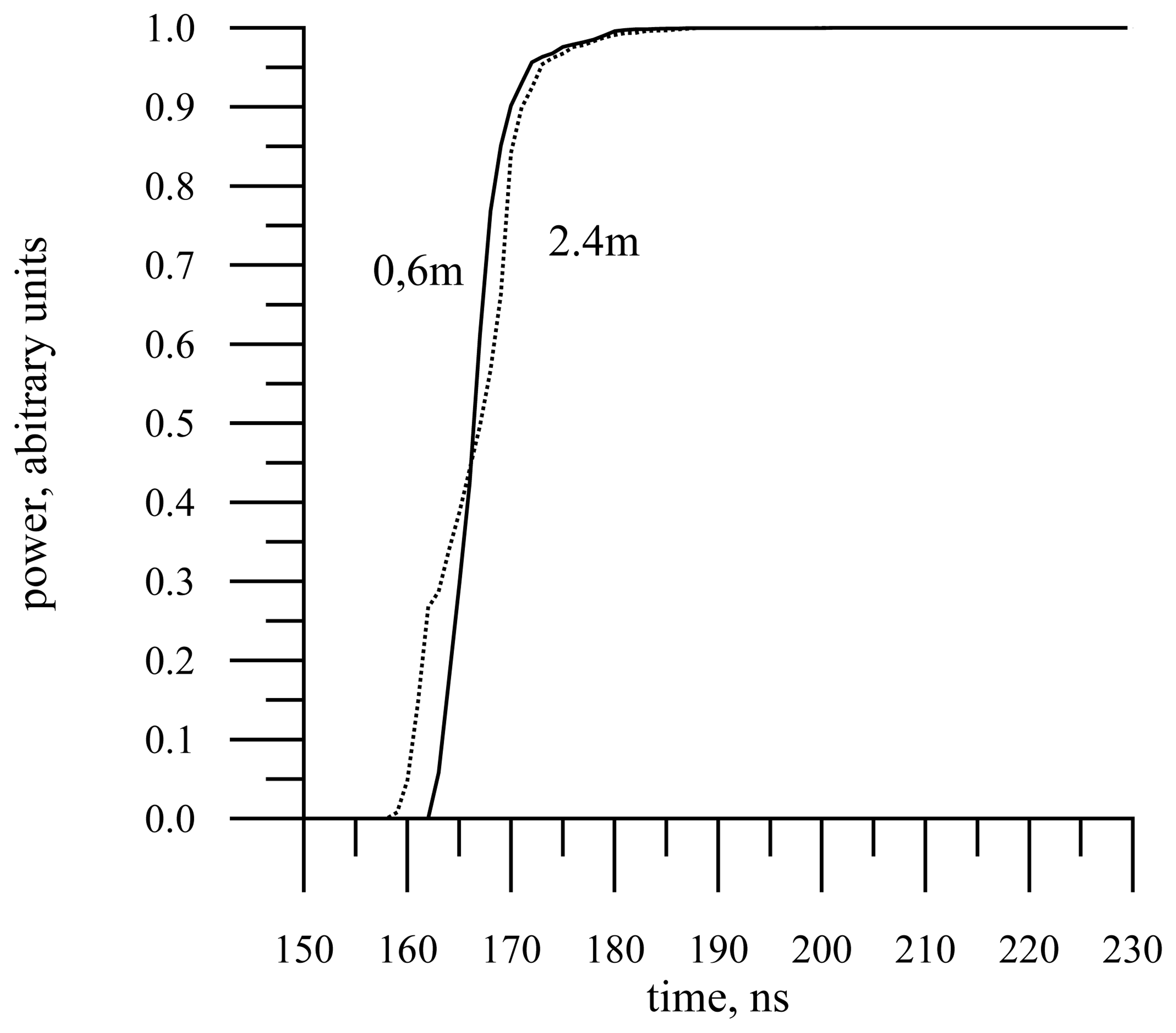
Fig.11 shows the sensitivity of the simulated reflected signal to significant wave height (for SWH equals 0.6m and 2.4m) for a Doppler filter corresponding to the velocity band 500-510m/s and a platform velocity of V = 8km/s.
Let us now consider what happens if the sea surface is moving. Assuming surface waves traveling towards the radar, the motion of the sea surface will increase̵s the Doppler shift and the reflected signal may occur earlier than in the case of an immobile surface.
The duration of the leading edge will depend on the significant wave height and the variance of orbital velocities, but significant wave height may be retrieved simply by measuring the slope of the leading edge close to the mid point of the leading edge. To calibrate the algorithm one may employ the significant wave height retrieved with the standard algorithm in the cell located directly under a satellite [
7,
15,
16]. The radar motion would make it possible to check the measurement accuracy of significant wave height in cells in the wide swath.
Obtaining the final algorithm to determine significant wave height off-nadir is beyond the scope of the present paper. Our aim here is simply to demonstrate a possible measurement principle. Quantitative assessments of the practical possibility to measure significant wave height in wide swath will be made in future.
9. Conclusions
Near-real time monitoring of the state of the ocean surface is a basis for solving numerous problems related to the safety of people's activities offshore and in coastal areas. Information is needed to draw up reliable weather forecasts and control global climate variations, and to understand the World Ocean.
Information is gathered by means of various scientific facilities, from buoys located in many important places of the World Ocean, to dedicated instruments mounted on satellites.
This paper presents the concept of the new radar system for measuring sea surface parameters over a wide-swath from a satellite. The following information on the state of the ocean surface can be retrieved: long waves slope variance, direction of large-scale wave propagation, near-surface wind speed. A slightly more elaborate version of the radar system would also enable significant wave height to be retrieved over a wide swath.
It is no detail description of radar system containing the answers at the technical questions but it is the first step in presentation of the new radar. It is theoretical analysis of opportunities of a new radar and the main goal of this presentation is attraction the attention of other researchers to new system and the first attempt to collect previous results together.
The essence of the suggested method relies on the use of a Doppler radar with a knife-beam antenna pattern rotating about the vertical axis.
If the radar system is mounted on a satellite, a wide swath is illuminated on the surface. For example, for an orbit height of 800 km and the antenna pattern 1°×25° the width of the swath for which reliable measurements can be obtained is 250 km. With further processing the footprint can be split into elementary scattering cells of the size, e.g. 14×14 кm. The roughness inside such cells may be assumed homogeneous and stationary. Previously developed algorithms are used to retrieve slope variance and the direction of wave propagation in each cell, as well as the wind speed. This two-dimensional image of the surface makes it possible to analyze wave processes on the ocean surface, to study their structure and temporal dynamics with repeated observations. To study small scale processes on the surface or in coastal areas, special algorithms can be applied to increase the spatial resolution, e.g., to operate with cells of the size 5×0.5 km.
