Integrating Remote Sensing Data with Directional Two- Dimensional Wavelet Analysis and Open Geospatial Techniques for Efficient Disaster Monitoring and Management

Abstract

In Taiwan, earthquakes have long been recognized as a major cause of landslides that are wide spread by floods brought by typhoons followed. Distinguishing between landslide spatial patterns in different disturbance regimes is fundamental for disaster monitoring, management, and land-cover restoration. To circumscribe landslides, this study adopts the normalized difference vegetation index (NDVI), which can be determined by simply applying mathematical operations of near-infrared and visible-red spectral data immediately after remotely sensed data is acquired. In real-time disaster monitoring, the NDVI is more effective than using land-cover classifications generated from remotely sensed data as land-cover classification tasks are extremely time consuming. Directional two-dimensional (2D) wavelet analysis has an advantage over traditional spectrum analysis in that it determines localized variations along a specific direction when identifying dominant modes of change, and where those modes are located in multi-temporal remotely sensed images. Open geospatial techniques comprise a series of solutions developed based on Open Geospatial Consortium specifications that can be applied to encode data for interoperability and develop an open geospatial service for sharing data. This study presents a novel approach and framework that uses directional 2D wavelet analysis of real-time NDVI images to effectively identify landslide patterns and share resulting patterns via open geospatial techniques. As a case study, this study analyzed NDVI images derived from SPOT HRV images before and after the ChiChi earthquake (7.3 on the Richter scale) that hit the Chenyulan basin in Taiwan, as well as images after two large typhoons (xangsane and Toraji) to delineate the spatial patterns of landslides caused by major disturbances. Disturbed spatial patterns of landslides that followed these events were successfully delineated using 2D wavelet analysis, and results of pattern recognitions of landslides were distributed simultaneously to other agents using geography markup language. Real-time information allows successive platforms (agents; to work with local geospatial data for disaster management. Furthermore, the proposed is suitable for detecting landslides in various regions on continental, regional, and local scales using remotely sensed data in various resolutions derived from SPOT HRV, IKONOS, and QuickBird multispectral images.

1. Introduction

Earthquakes have long been recognized as a major cause of landslides [1]. However, landslides are only the first in a series of processes by which materials can be removed from slopes and transported out of a region by fluvial action [2]. In Taiwan, typhoons that unleash massive amounts of rainfall hit Taiwan every year between July and October. Since 1999, after the ChiChi earthquake, the expansion rate of landslide areas has grown 20 times in central Taiwan [3] due to the numerous extension cracks, which accelerate landslides during downpours, generated on hill slopes during the ChiChi earthquake [4]. Landslide monitoring, management, and land-cover restoration have become high priority tasks that reduce damage to livelihoods and economies. However, landslides monitoring via field surveys is time consuming because of the widespread distribution of landslides and limited accessibility to disaster regions. Remotely sensed data has become an efficient means of quantifying the spatial characteristics of landscape changes both regionally and globally [5].

The conventional approaches for landslide inventory using remotely sensed data encompass scar interpretations ranging from visual to semi-automatic interpretations of aerial photographs and land-cover classifications ranging from per-pixel to objective land-cover classifications of spectral images [6]. Such interpretations and classifications for landslide identifications are time-consuming procedures that cannot meet urgency of disaster monitoring and management. An alternative approach is to utilize the normalized difference vegetation index (NDVI) as a rapid inferential index for landslide identification [6]. As NDVI images can be determined by simple geometric operations of near-infrared and visible-red spectral data immediately after remotely sensed data is acquired. The NDVI has become the most common vegetation index, and has been extensively applied to assess the vigor of plants [7]. Significant differences of NDVI variations in images before and after a natural disturbance can be landslides induced by a disturbance that alters land from covered with plants to bare land.

Wavelet analysis, which can determine localized variations in NDVI, is closely related to the windowed Fourier analysis, except that wavelet analysis involves adjustable filtering banks to deal with localized variations filtered out by moving a filtering bank to a specific location in the spatial domain [8]. Wavelet analysis can be categorized as continuous and discrete based on parameters. Continuous wavelet analysis is more flexible than discrete wavelet analysis and is frequently preferred due to its efficiency in extracting signal information from data at a specific scale [9]. Among the various continuous two-dimensional (2D) wavelet functions, the Gaussian wavelet functions, such as the Morlet wavelet function, have the smallest bank size [10]. The Morlet wavelet function is superior in scale detection and localization to other wavelet functions [11]. That the Morlet wavelet function can utilize a filtering bank to filter out localized variations along particular directions is termed a ′directional′ characteristic. Such characteristic is suitable for detecting spatial features with a declination angle [12].

Although remotely sensed data is widely used by governmental agencies, data interoperability and exchangeability are still common problems. An information center must provide real-time spatially interpretable data to decision-making agencies for disaster management and deliver interoperable and exchangeable data to successive disaster reduction units to work with local geospatial data for subsequent restoration tasks. A standard solution for interoperability and exchangeability is necessary for disaster monitoring, management, and land-cover restoration and to utilize local data in a global application that performs global processing and synthesizing. The Open Geospatial Consortium (OGC) developed an extensible markup language (XML)-based standard called the geography markup language (GML) for dealing with geospatial data. The GML has already been employed as an encoding scheme for exchange of geospatial data, a modeling language for describing geospatial information, and as a storage format. The GML also construct a fabric interconnection of geospatial data sets and services in the World Wide Web much as hypertext markup language (HTML; has done for text-based information [13]. Great potential exists for by GML to integrate rich geospatial data with updates of disaster impact and resource deployment for disaster monitoring, management, and land-cover restoration.

This study integrates the directional 2D Morlet wavelet analysis with NDVI images to instantly identify potential landslide sites. The directional 2D wavelet analysis was illustrated by artificial point patterns. Field data for NDVI images were derived from SPOT HRV images before and after the ChiChi earthquake (7.3 on the Richter scale) in the Chenyulan basin of Taiwan, as well as images after two large typhoons, Xangsane and Toraji. These images were analyzed to determine the spatial patterns of landslides caused by these major disturbances. Spatial patterns of landslides in different disturbance regimes are discussed. Implementation of the system architecture for simultaneous distribution of analytical results to other agencies by GML is illustrated. Possible applications on the Internet and mobile devices, and compliant data for the proposed framework are also discussed.

2. Methods and Materials

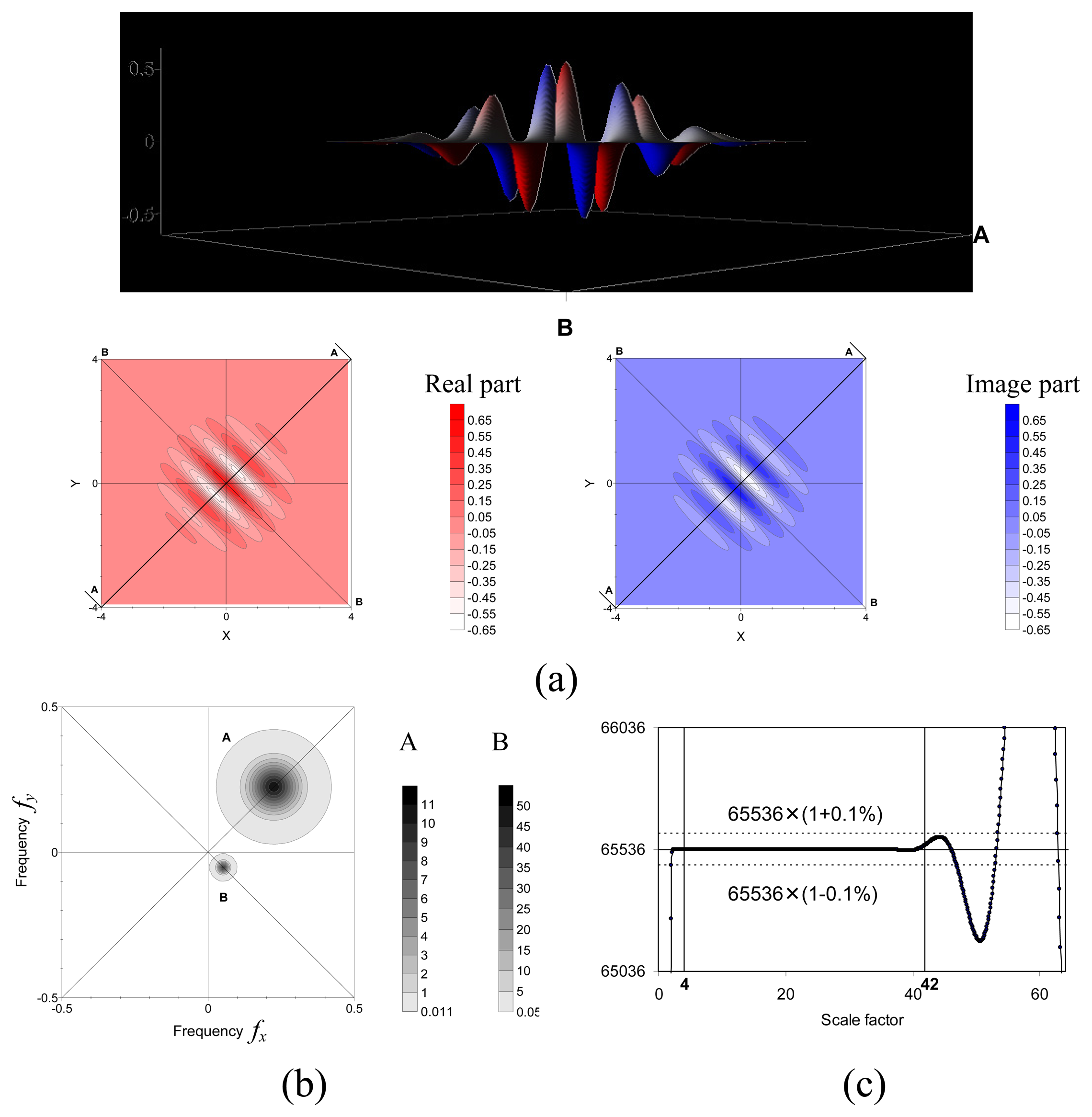
2.1. Directional 2D Morlet wavelet analysis

The 2D Morlet wavelet function is given by [7]

$$\phi \left(\stackrel{\rightharpoonup }{r},\theta \right)={\pi }^{-0.5}{e}^{-\stackrel{\rightharpoonup }{{\omega }_0}(\theta )\cdot \stackrel{\rightharpoonup }{r}}{e}^{-0.5{\left|\stackrel{\rightharpoonup }{r}\right|}^2},$$

(1)

where r⃑ is a location vector; $\stackrel{\rightharpoonup }{{\omega }_0}\left(\theta \right)=\left({\omega }_{0x}(\theta ),{\omega }_{0y}(\theta )\right)=\left(\left|\stackrel{\rightharpoonup }{{\omega }_0}\right|cos(\theta ),\left|\stackrel{\rightharpoonup }{{\omega }_0}\right|sin(\theta )\right)$ is a directional vector, that is taken to be six in this study to satisfy the admissibility condition [11], and the directional angle θ is positively measured counter-clockwise from due east with a range of π/2 ≥ θ > − π/2. The dilated φ(r⃑) is defined as

$${\phi }_{\lambda }\left(\stackrel{\rightharpoonup }{r},\theta \right)=\frac{{\pi }^{-0.5}}{\lambda }{e}^{-i\stackrel{\rightharpoonup }{{\omega }_0}(\theta )\cdot \frac{\stackrel{\rightharpoonup }{r}}{\lambda }}{e}^{-0.5{\left|\frac{\stackrel{\rightharpoonup }{r}}{\lambda }\right|}^2},$$

(2)

where λ is a scale factor and the normalized constant $\frac{1}{\lambda }$ is chosen to conserve the norm so that $\int {\left|{\phi }_{\lambda }\left(\stackrel{\rightharpoonup }{r},\theta \right)\right|}^{2}d\stackrel{\rightharpoonup }{r}=\int {\left|\phi \left(\stackrel{\rightharpoonup }{r},\theta \right)\right|}^{2}d\stackrel{\rightharpoonup }{r}$. By setting $\left|\stackrel{\rightharpoonup }{{\omega }_0}\right|=6$, θ = 4/, and λ = 1, the real, Re(φ_λ(r⃑, θ)), and image, Im(φ_λ(r⃑, θ)), parts of φ_λ(r⃑, θ) are illustrated in Figure 1(a).

Data of variable Z(r⃑) is obtained from the study area, Ω, composed of N_x × N_y grid nodes. The Morlet wavelet transform of Z(r⃑) is defined by the convolution of Z(r⃑) and the conjugate of the wavelet function, φ_λ(r⃑), as

$$WZ=\left(\stackrel{\rightharpoonup }{r},\lambda ,\theta \right)=\int g\left(\stackrel{\rightharpoonup }{u}\right){\phi }_{\lambda ,\stackrel{\rightharpoonup }{r}}^{*}\left(\stackrel{\rightharpoonup }{u},\theta \right)d\stackrel{\rightharpoonup }{u},$$

(3)

where u⃑, r⃑ ∈ Ω are location vectors; ${\phi }_{\lambda ,\stackrel{\rightharpoonup }{r}}^{*}\left(\stackrel{\rightharpoonup }{u},\theta \right)={\phi }_{\lambda }^{*}\left(\stackrel{\rightharpoonup }{u}-\stackrel{\rightharpoonup }{r},\theta \right)$ and ′*′ indicates the complex conjugate. According to the Parseval′s relation [3], WZ(λ, r⃑) can be written as

$$WZ\left(\stackrel{\rightharpoonup }{r},\lambda ,\theta \right)=F^{-1}\left(FZ\left(\stackrel{\rightharpoonup }{f}\right)F{\phi }_{\lambda ,\stackrel{\rightharpoonup }{r}}^{*}\left(\stackrel{\rightharpoonup }{f},\theta \right)\right),$$

(4)

where F and F⁻¹ represent the Fourier transform and the reverse Fourier transform, respectively; f⃑ = (f_x, f_y)is a frequency.

The Fourier transform of φ*(r⃑, θ), Fφ* (f⃑, θ), is a shifted Gaussian with its center at $\stackrel{\rightharpoonup }{w_0}$ as

$$F{\phi }^{*}\left(\stackrel{\rightharpoonup }{f},\theta \right)=2\pi \left({\pi }^{-0.5}{e}^{\frac{{(2\pi f_x-w_{0x}(\theta ))}^2+{(2\pi f_y-w_{0y}(\theta ))}^2}{2}}\right),$$

(5)

where ${\int \left|F{\phi }^{*}\left(\stackrel{\rightharpoonup }{f},\theta \right)\right|}^{2}d{f}_{x}d{f}_y=1$. A wavelet function is directional if its Fourier transform is a convex cone with the apex deviating from the origin in the frequency domain [12]. For each scale λ, the Fourier transform of ${\phi }_{\lambda }^{*}\left(\stackrel{\rightharpoonup }{u}\right)$ is

$$F{\phi }_{\lambda }^{*}\left(\stackrel{\rightharpoonup }{f},\theta \right)=2\lambda \sqrt{\pi }{e}^{\frac{{\lambda }^2}{2}\left[{\left(2\pi f_x-\frac{w_{0x}(\theta )}{\lambda }\right)}^2+{\left(2\pi f_y-\frac{w_{0y}(\theta )}{\lambda }\right)}^2\right]},$$

(6)

with its center at $\stackrel{\rightharpoonup }{w_0}\left(\theta \right)/\lambda$. The discrete summation of the norm of $F{\phi }_{\lambda }^{*}\left(\stackrel{\rightharpoonup }{f},\theta \right)$has the property of

$$\text{∑}_{f_x}\text{∑}_{f_y}{\left|F{\phi }_{\lambda }^{*}\left(\stackrel{\rightharpoonup }{f},\theta \right)\right|}^2=N_x{N}_y,$$

(7)

that makes the wavelet transform be weighted neither by the wavelet function nor the scale factor. According to Equations (7) and (4), the wavelet mean spectrum over the study area, $\overline{{\left|WZ\left(\lambda ,\theta \right)\right|}^2}=\text{∑}_{\stackrel{\rightharpoonup }{r}}{\left|WZ\left(\stackrel{\rightharpoonup }{r},\lambda ,\theta \right)\right|}^2/\left(N_x{N}_y\right)$, for a spatial randomness is equal to N_xN_y times the expectation value of ∣FZ(f⃑)∣², and is equal to the square mean of the original data as $\text{∑}_{N_x}\text{∑}_{N_y}{Z}^2/\left(N_x{N}_y\right)$ [3]. The mean spectrum of the wavelet analysis of any data set can be normalized by the square mean of the original data to show how original data deviates from randomness, while the expectation value of the normalized mean spectrum for a spatial randomness is equal to one.

The phase of φ(r⃑, θ) is defined as tan⁻¹ (Im(φ(r⃑, θ))/Re(φ(r⃑, θ))), and the iso-phase lines are perpendicular to the directional vector $\stackrel{\rightharpoonup }{w_0}\left(\theta \right)$. The wavelet transform decomposes the variation of Z by the filtering bank into elements with periodically changing phases along the directional vector [8].The detecting direction in wavelet analysis is defined by the choice of the directional vector, $\stackrel{\rightharpoonup }{w_0}\left(\theta \right)$, that varies with the directional angle, θ. Figure 1(b) shows the Fourier transforms of the conjugate of the Morlet wavelet function with different scale factors and directional angles.

The range of scale factors λ that can be applied in a wavelet transform depends on the number of grid nodes in the study area. The minimum value of the scale factor, λ_min, is chosen so that the maximum shift of the center in the Fourier transform of ${\phi }_{\lambda }^{*}\left(\stackrel{\rightharpoonup }{u},\theta \right),\left|\stackrel{\rightharpoonup }{w_0}\left(\theta \right)\right|/{\lambda }_{min}$, does not excess the Nyquist frequency, 2π∣f⃑∣_max/2. Because ∣φ_λ(u⃑, θ)∣ decays to 0.01∣φ_λ(0,θ)∣ at ∣u⃑∣ = 3λ, the maximum value of the scale factor, λ_max, is chosen by 3λ_max≤ min (N_x, N_y)/2 so that that all values of ∣φ_λ(u⃑, θ)∣ being greater than 0.01∣φ_λ(0, θ)∣ should be contained in the study area [14]. By setting N_x=N_y = 256, maximum 1integral value of λ_max is 42 (3λ_max ≤ 256/2), while the minimum integral value of λ_min is four (6/λ_min≤ 2π × 0.5/2). According to Equation (7), determination of ${\text{∑}_{f_x}\text{∑}_{f_y}\left|F{\phi }_{\lambda }^{*}\left(\stackrel{\rightharpoonup }{f},\theta \right)\right|}^2$ is N_xN_y × (1±0.1%) in the scale range determined, as shown in Figure 1(c).

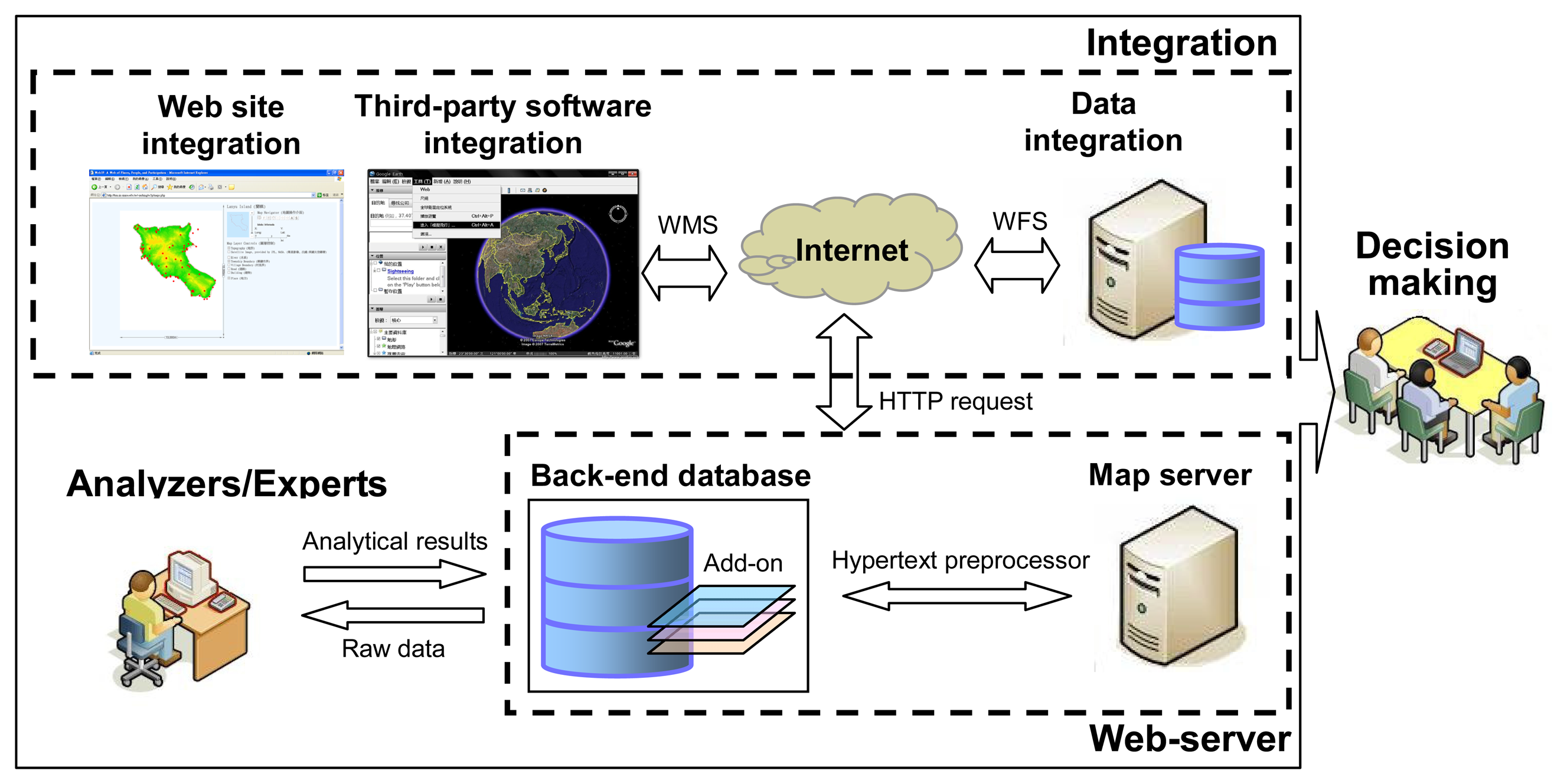
2.2. System architecture for rapid information sharing

A back-end database is utilized for storing and handling geospatial data (e.g., PostgreSQL and GRASS), while an accompanied add-on deals with geospatial data using spatial operations (e.g., PostGIS). Experts or analysts can easily retrieve raw geospatial data from a database to detect landsides and update the database with analytical results. A hypertext preprocessor (e.g., PHP) connects a web server (e.g., Apache) and back-end database, whereas a map server (e.g., Mapserver) conjugating the web server serves as a common gateway interface (CGI) for geospatial data requests from clients. The CGI implements protocols, termed web map service (WMS) and web feature service (WFS), developed by the OGC that allows end users to retrieve geospatial data via a hypertext transmission protocol (HTTP) request. The WMS allows clients to overlay map images retrieved from multiple sources for display on the Internet [15], whereas the WFS allows clients to retrieve and update geospatial data encoded in GML [16]. Via this architecture, clients can utilize map images and attributes of spatial features maps gathered from different sources (Figure 2).

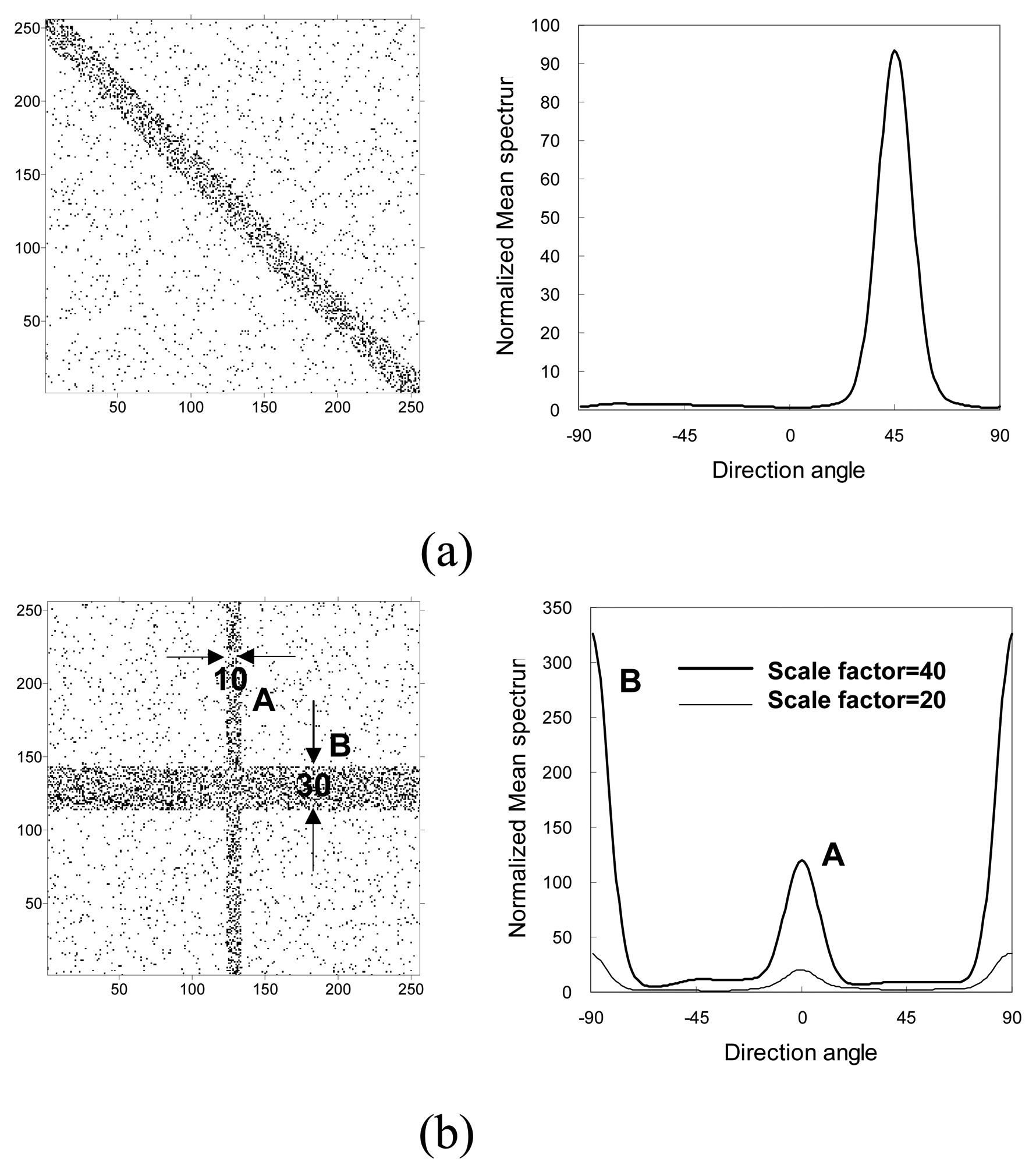
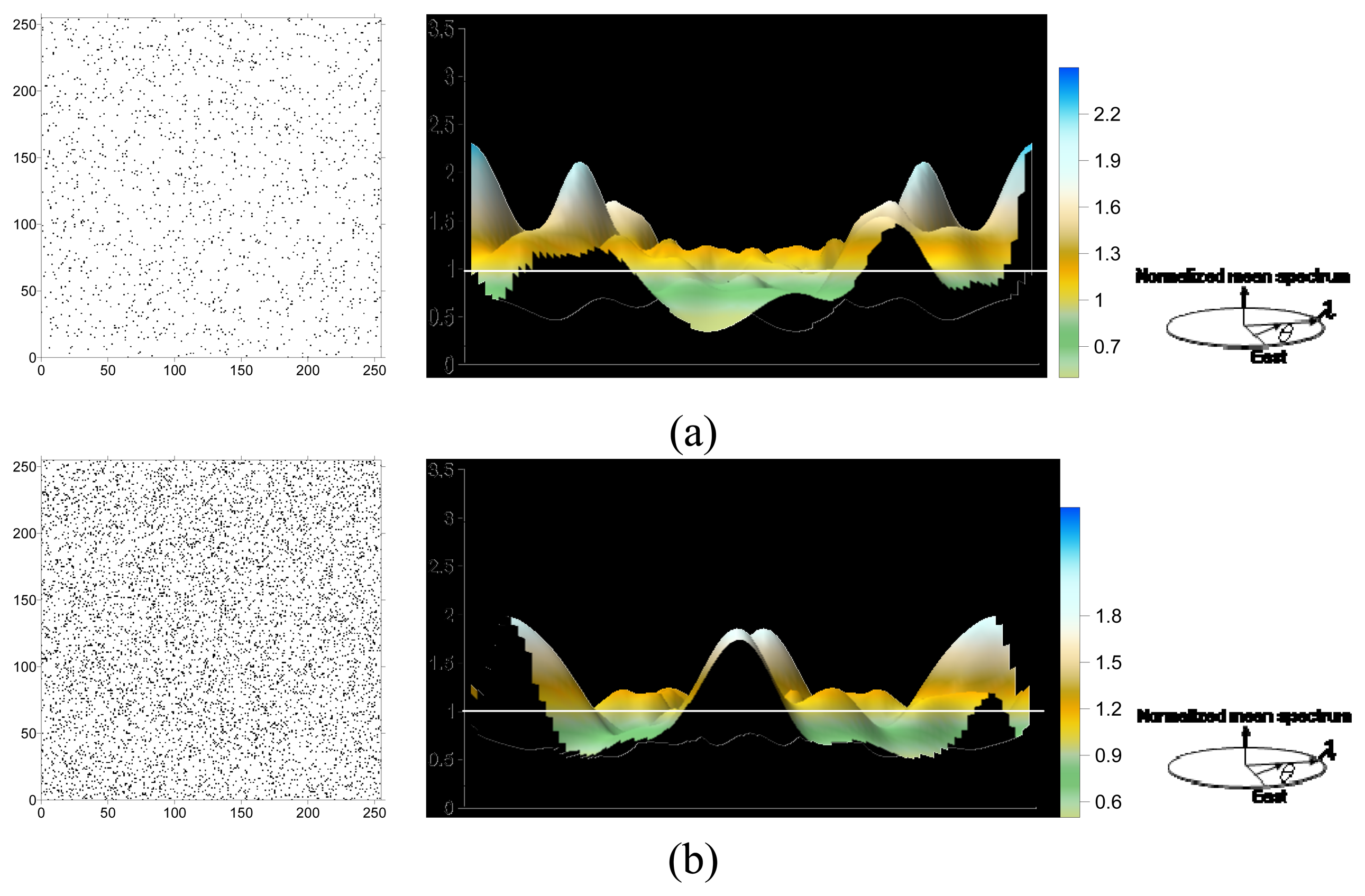
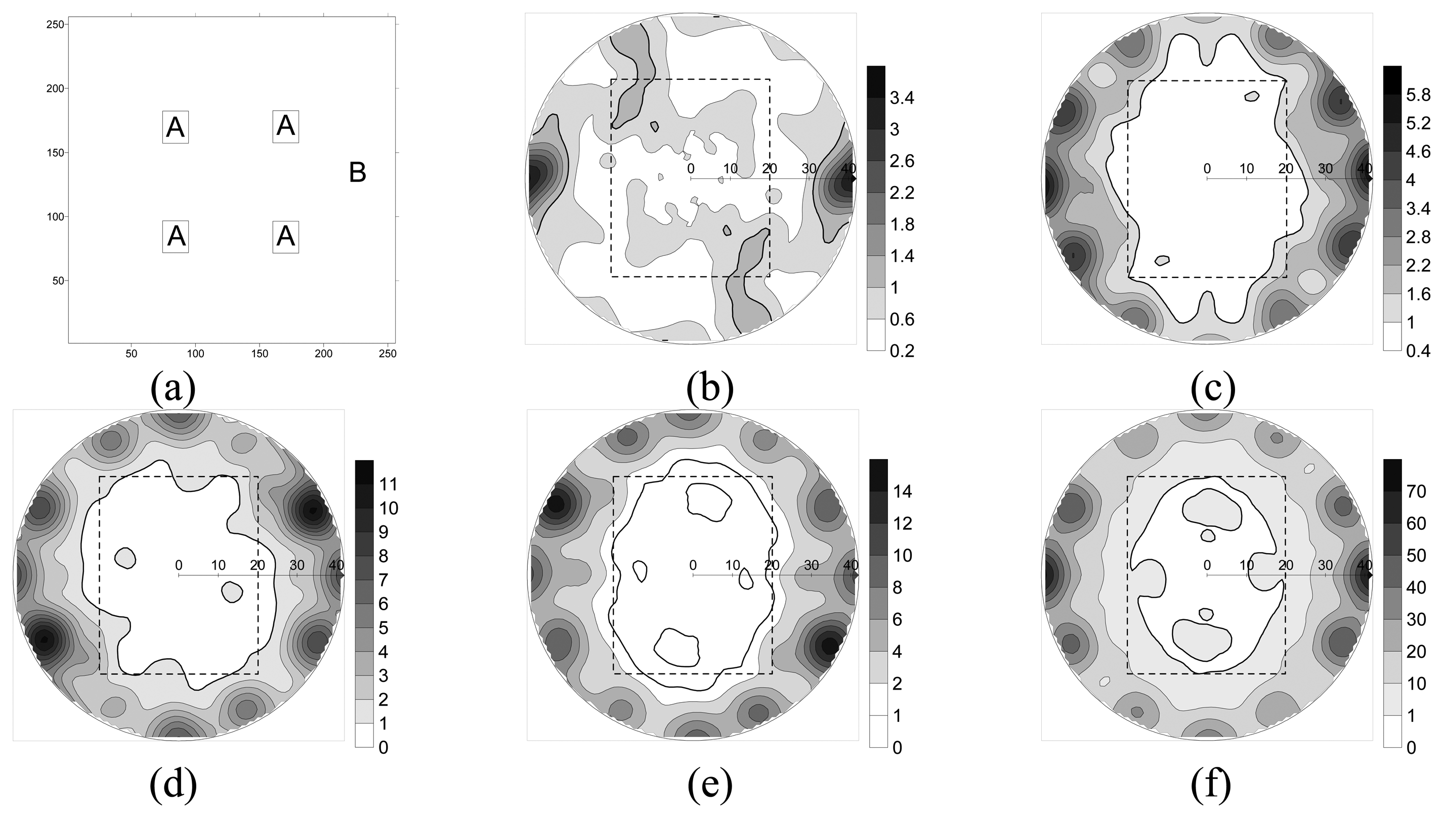
2.3. Artificial data

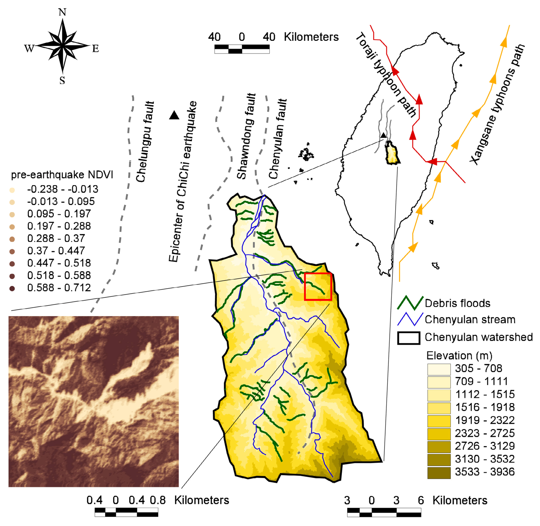
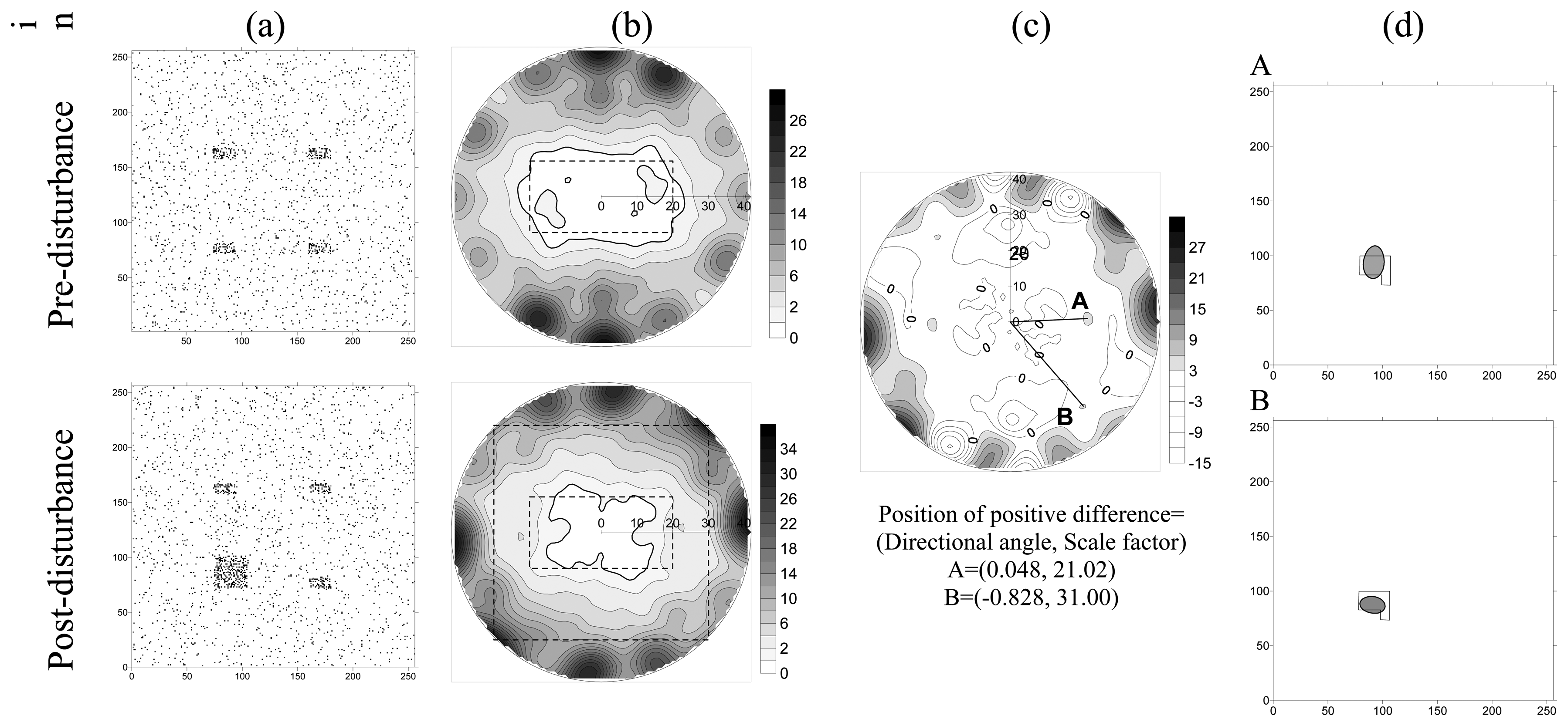
Wavelet analysis, which was originally developed for analyzing continuous datasets, can also be applied to point data [17]. The directional 2D wavelet analysis is demonstrated using artificial point patterns ranging from random to obvious patterns of clumps with a specific aspect radio to confirm its performance in separating true patterns from random fluctuations. The mean spectrum is normalized using the square mean of original data, and an envelope of the normalized mean spectrum generated from 100 simulated random replicates is used to determine the significance of simulated data deviating from spatial randomness. As Morlet wavelet analysis can filter out variations in data on various scales with multiple directions; the mean spectrum is a function of scale factor and directional angle as $\overline{{\left|WZ\left(\lambda ,\theta \right)\right|}^2}$. Simulations are calculated over multiple replications and various scales and directions, and mean spectrums are depicted in a spectrum map against scale factors in the radial direction and directional angles in the angular direction. Belt patterns with different declinations and widths are also used to confirm the ability of directional 2D Morlet wavelet analysis to detect dominant spatial pattern scales and angles]. Two artificially clumped point patterns with different clump sizes at a predefined location were generated to simulate landslide expansion induced by a disturbance. Wavelet analysis is applied to detect the location at which significant changes occurred and determine how these changes occurred in scales and directions.

2.4. Field data

Field data were collected from the Chenyulan watershed. The Chenyulan watershed, located in central Taiwan, is an intermountain watershed, and has average altitude of 1540 m and area of 449 km². The Chenyulan stream which follows the Chenyulan fault flows from south to north and elongates the watershed in the same direction. Different uplifting along the fault has generated abundant fractures throughout the watershed, resulting in an average slope of 62.5% and relief of 585 m/km² in the watershed. Moreover, the main course of the Chenyulan stream has a gradient of 6.1%, and over 60% of its tributaries have gradients exceeding 20%. The special geological and geographical characteristics of the watershed result in frequent landsides and debris flows [18]. At 01:47′12.6″ on Sep. 21, 1999, the ChiChi earthquake (7.3 on the Richter scale), caused by motion of the Chelungpu thrust fault, struck central Taiwan. The earthquake epicenter was located at 23.87°N and 120.75°E, around 30 km north-northwest of the Chenyulan watershed [19]. One year the earthquake, typhoon Xangsane brushed the eastern side of the watershed as it moved from south to north and dropped 127-270 mm of total rainfall in the watershed between Oct. 31, and Nov. 1, 2000 [20]. Another typhoon, Toraji, which brought intense rainfall over a short duration exceeding 300 years return period, hit the watershed as it moved east to west on July 28-31, 2001. After crossing Taiwan, typhoon Toraji degraded into a tropical storm; however, the typhoon dropped 339-757 mm of rainfall in the watershed [21]. Sediments already loosened by the ChiChi earthquake bore the torrential rainfall brought by the two typhoons. Consequently, a large quantity of loose sediment promoted massive debris flows during subsequent typhoons. The Taiwan Water and Soil Conservation Bureau announced debris flood warnings for several tributaries of the Chenyulan stream after typhoon Toraji. Location of landslides was shifted from mid-hills to hilltops in central Taiwan by the ChiChi earthquake, and hilltop landslides triggered serious debris flows [22]. The study area 3.2×3.2 km² (256×256 pixels) was selected upstream of the largest debris flood in the watershed (Figure 3).

The NDVI images of the study area were generated from the SPOT HRV images with resolution of 12.5 m using the following equation:

$$\text{NDVI}=\frac{(\text{NR}-\text{R})}{(\text{NIR}-\text{R})},$$

(8)

where NIR and R are near-infrared and visible-red spectral data, respectively. The NDVI values range from −1 to +1; a higher NDVI value indicates that an area has a large amount of high photosynthesizing vegetation [7]. The pre-earthquake NDVI image, generated on March 6, 1999, before the ChiChi earthquake was utilized as a datum image for radiometric corrections between different radiometric conditions in multi-temporal images of the Chunyulan watershed. To eliminate seasonal effects, three post-earthquake NDVI images were generated during late Oct. to early Nov., and on Oct. 31, 1999, after the ChiChi earthquake, Nov. 27, 2000, after the Xangsane typhoon, and Nov. 20, 2001, after the Toraji typhoon. Four NDVI images were chronologically denoted as Stages 1 to 4. Fifty control points, which were identified as unchanged in all images, were used to establish the linear regression for post-earthquake images to the datum image.

$${\mathbf{\text{X}}}_i=a{\mathbf{\text{X}}}_d+b$$

(9)

where X_i is a matrix composed of NDVI values of 50 control points at stage i; X_d is a matrix composed of NDVI values of 50 control points at the datum image; a and b are coefficients.

3. Results and Discussion

3.1. Artificial data

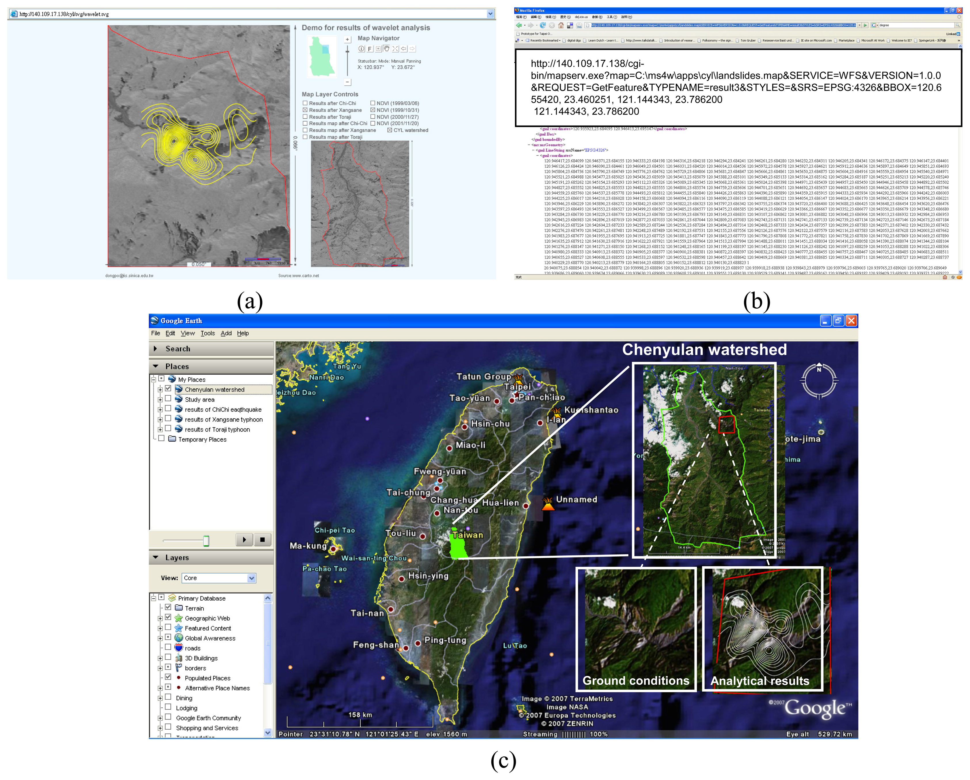
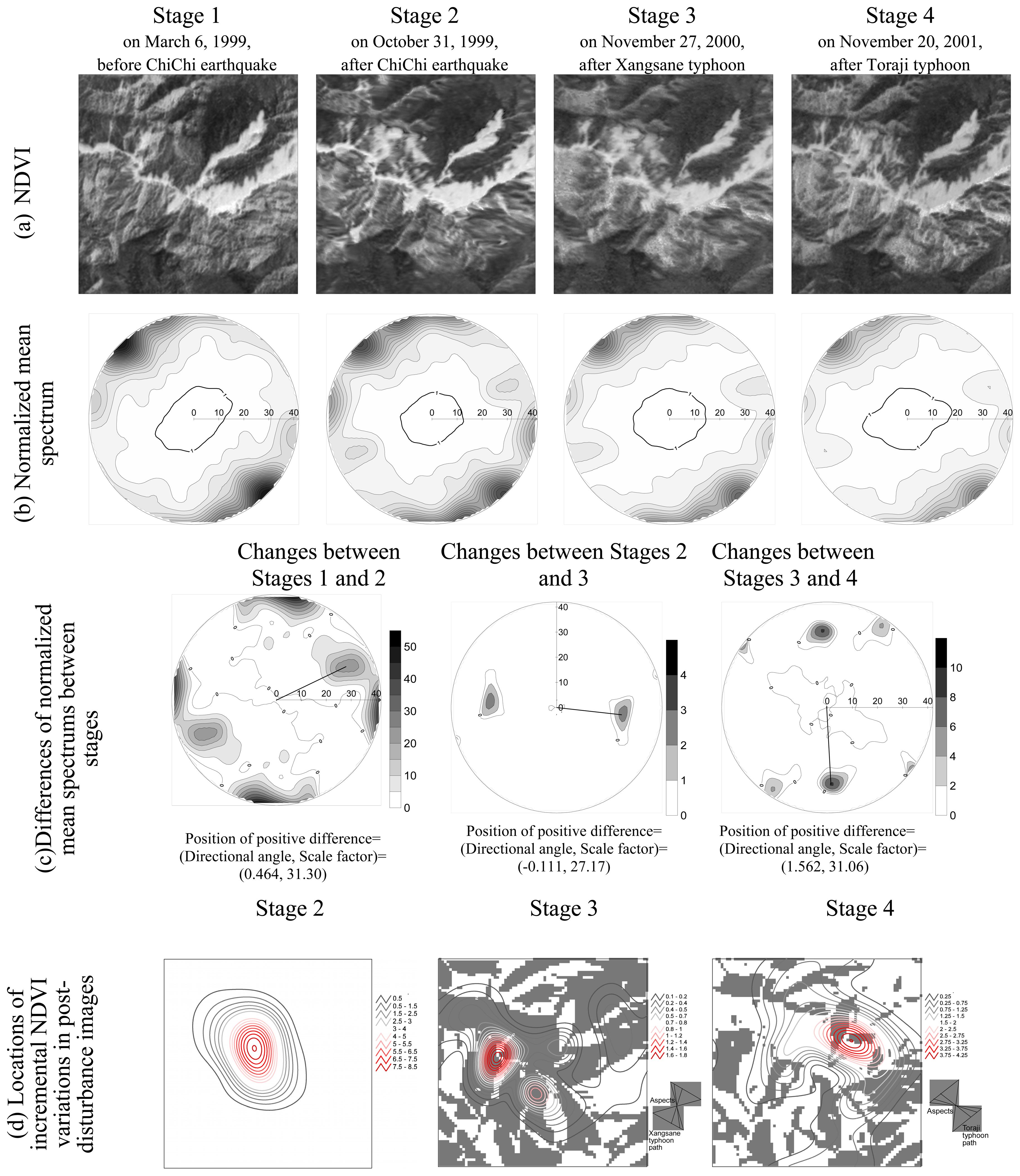
Two spatially random point patterns with point densities of 0.025 (1639/65536) and 0.1 (6554/65536) were generated (Figure 4). The spectrum map of those two patterns were normalized using the square mean of original data, $0.025(\text{∑}_{1639}{1}^2/65536)$ and 0.1 $(\text{∑}_{1639}{1}^2/65536)$. Normalized mean spectrums fluctuated randomly around a value of one in the envelope (range, 0.23-2.96). The expected value of normalized mean spectrum for a spatial randomness is one. And the envelope was generated from 100 duplicates of spatially random point patterns.

Point clumps with different densities were generated in 4 regions with an area of 20 × 25 grid nodes for each on a random background with an area of 256 × 255 grid nodes (Figure 5(a)). The background randomness has a point density of 0.025 (1639/65536), whereas point clumps have 2-, 4-, 6-, 8-, and 24-fold point densities relative to the background. Spectrum maps were employed to assess the performance of the directional 2D Morlet wavelet analysis in separating true patterns from random fluctuations. Mean spectrums in the spectrum maps were normalized using the square mean of background randomness, $\mathrm{0(025}(\text{∑}_{1639}{1}^2/65536)$. As a point density in a clump increases, the number of points in clumps that are restricted increases. As the number of random points decreases, the degree to which a normalized mean spectrum deviates from one increases; one is the expected value of a normalized mean spectrum for a spatial randomness. As the density in clumps increases, the strength of a pattern increases both visually and analytically (Figures 5(b)–(f)). Clumps with 8-fold point density relative to the background are visually recognizable in a spectrum map (Figure 5(e)).

A belt pattern with a declination of −π/4, width of 20 grid nodes and a crucifix pattern composed of two belts with widths of 30 and 10 grid nodes and respective declinations of zero and π/2 were generated. The normalized mean spectrums on a specific scale were diagramed against directional angles. Figure 6(a) presents the mean spectrum on a scale factor of 30, the largest normalized mean spectrum identified in the direction perpendicular to the declination angle, π/4, along which the maximum variation in the point pattern occurred. For the crucifix pattern, the normalized mean spectrum on a scale factor of 40 is the largest at a directional angle of π/2 for the thick belt with a width of 30 grid nodes and declination of zero. The largest normalized mean spectrum for the thin belt is at a directional angle of zero, and this value is markedly smaller than that of the thick belt. However, as the scale factor for wavelet analysis decreases from 40 to 20, smaller than the width of the thick belt and larger than the width of the thin belt, the largest normalized mean spectrums between thick and thin belts are the same (Figure 6(b)). Analytical results indicate that the pattern of point clumps is distinguishable only when the scale of the filtering bank in wavelet analysis is larger than clump sizes. These simulations demonstrate that directional 2D Morlet wavelet analysis is efficient in detecting dominant scales and angles in a spatial pattern.

Two artificially clumped point patterns with different clump sizes at a predefined location were generated to simulate expansion of a landslide induced by a disturbance (Figure 7(a)). The respective normalized mean spectrums were determined (Figure 7(b)) and the increase in the normalized mean spectrums in the post-disturbance pattern relative to the pre-disturbance pattern were identified by scale factors and directional angles (Figure 7(c)). The localized spectrums determined by setting the filtering bank based on identified scale factors and directional angles were calculated for each grid of the post-disturbance pattern to identify the location at which a significant increment of point variation occurred. The coincidence between pre-defined and identified locations (Figure 7(d)) indicates that the localization characteristic makes directional 2D Morlet wavelet analysis a powerful tool for locating significant differences between two patterns.

3.2. Field data

between Stages 1 and 2, typhoon Xangsane between Stages 2 and 3, and typhoon Toraji between Stages 3 and 4, the NDVI variations are considered mainly caused by these large natural disturbances. The dominant scale factor and directional angle of landslide patterns induced by natural disturbances were identified by the most significant differences in NDVI variations between stages (Figure 8(c)). The dominant scales and directional angles were 31.3 and 0.46, 27.2 and −0.11, and 31.1 and 1.52 for the ChiChi earthquake, typhoon Xangsane, and typhoon Toraji, respectively. The dominant scale of NDVI variations induced by typhoon Toraji is larger than that induced by typhoon Xangsane, probably due to the fact that typhoon Toraji brought relatively more amount and stronger intensity of rainfall. The filtering banks in wavelet analysis were set according to the identified dominant scales and directional angles to determine localized variations surrounding each grid in post-disturbance images (Figure 8(d)). The spatial distribution of incremental NDVI variations at Stage 3 relative to Stage 2 and at Stage 4 relative to Stage 3 combined with hill aspects were used to identify the orographic effects due to interactions between typhoons and mountain topography. High NDVI variations existed on hillsides with hill aspects within ±π/4 aligned with typhoon paths.

3.3. Open GIS

Figure 9(a) presents a snapshot of the interface implemented by GML-compliant language (e.g., scalable vector graphics or SVG) allowing clients to browse analytical results on the Internet using a web browser. Figure 9(b) shows the WFS request for analytical results. The GML document is a document that can be opened by any generic web browser via an HTTP request. Thus, data can be distributed worldwide instantly. In addition to using a web browser, end users can use the WMS/WFS complaint applications, such as Google Earth, to request maps via the Internet (Figure 9(b)). Many commercialized GIS applications have also been implemented to handle GML documents (e.g., Tatuk GIS). The prototype in this study is a way of overcoming difficulties by rapidly integrating heterogeneous data and efficiently transporting disaster information via open geospatial technologies.

3.4. Discussion

Traditional landslide identification based on land-cover classifications adopts data, including spectral data, geomorphometric data, vegetation data, and geometric shapes of landslides gathered at a specific time after a disturbance [6]. The proposed method, which is based on detecting changes before and after a disturbance, identified significant differences in NDVI variations generated by natural disturbances. Using NDVI images for landslide identification is only suitable for images acquired immediately after a disturbance as old landslide events may have been subject to re-vegetation and may lead to erroneous delineation of landslides [6]. Significant differences in NDVI values rather than NDVI variations determined by simple subtraction of NDVI images can also be utilized for landslide identification [23]. However, spatial characteristics of area extent of landslides are valuable for disaster management, such as dominant scales, and can be synchronously obtained using directional 2D Morlet wavelet analysis rather than simple subtraction. Monitoring restoration activities plays a key role in determining end points for restoration and assessing effectiveness. Appropriate monitoring of major systems, particularly in assessing vegetation reestablishment, requires a long-term commitment to annual assessment of change and improvement over time [24]. The framework in this study can help assess the restoration success by extracting spatial information from NDVI imageries.

Adopting temporal differences in images for landslide identification should consider temporal heterogeneity of radiometric conditions in multi-temporal images that are affected by ground conditions, atmospheric conditions, and illumination effects [25]. An empirical radiometric correction shifts the spectral data in a destination image to the datum image by linear regression based on identifying unaltered objects between images. Moreover, change detection via a comparison between images is meaningful only when both images have the same energy density (spectrum). The square mean of NDVI values for a spatial randomness is proportion to the disturbance spectrum [26], and was adopted to normalize the determined wavelet spectrum to determine the significance of normalized wavelet spectrum deviating from spatial randomness. By decomposing and allocating the same sum of squared NDVI values into different spatial distributions over the study area, the normalized procedure helps discriminate between different spatial patterns induced by different natural disturbances.

Landslides induced by earthquakes and typhoons have distinct spatial patterns. Typhoons can significantly influence NDVI variations via the flow of accumulated rainfall and wind gradients. Disturbances induced by typhoons can be explained by simple exposure relationships between slope, aspect, and wind direction [27]. Variations in the NDVI induced by typhoons are therefore anisotropic and in accordance with topographical exposures. However, disturbances associated with earthquakes are not regularized by topography in the same way as they are by typhoons. Variations to the NDVI generated by earthquakes are thus more isotropic than those generated by typhoons. Analytical results generated by the directional 2D Morlet wavelet analysis identified coincident phenomena in that NDVI variations generated by earthquakes are more isotropic than those generated by typhoons (Figure 8(b)).

The proposed method is designed to analyze the landscape mosaic induced by natural disturbances, and thus identifies the location and area extent of clustered landslides rather than the distinct shape and area of a single landslide. Because the modulus of the wavelet transform, ∣WZ(λ, θ)∣², determines the local variation around a grid. For an end-user who concerns the exact boundary of the landslides, the modulus of wavelet transform can be substituted into the existing algorithm for edge detecting like Canny algorithm that calculates the maximum wavelet modulus at an edge [28]. The wavelet function have to be directional like Gabor or spline dyadic wavelets [28, 29]. The dominant scale factors are dimensions that illustrate how clustered landslides expand, whereas the dominant directional angles identify the direction in which those landslides were aligned. Landslide initiation is determined by static and dynamic factors. Static factors describing bearing capacity include geomorphology and land-cover, whereas dynamic factors describing triggers of mass movement include hydrological and perturbation conditions [30]. A strong trigger generates a large determinant scale factor for clustered landslides and an intensive NDVI variation (Figure 8(c)). As the anisotropic characteristics of landslides vary with different disturbances, the dominant directional angles identified by directional wavelet analysis vary with different disturbances. Typhoons always generate more recurrent changes along an exposure aspect aligned with the typhoon path, and abrupt changes perpendicular to the aspect. Therefore, the spatial distribution of significant differences in NDVI variations should be located on a terrain with aspects exposed to a typhoon, and along side banks of gullies that are prone to accumulate rainfall (Figure 8(d)).

Wavelet analysis was adopted in this study to identify the abrupt variation in the NDVI across the edge between bare land and that covered with plants. Landslides in images are features with declination angles. Flat NDVI variations are along the declination direction, whereas abrupt NDVI variations are along the perpendicular direction. Tasks in landslide identification become edge detection problems. Many techniques have been developed for edge detection, which is a classical problem in image processing. If oriented features are detected, a wavelet function that is directionally selective is required [9, 12]. In addition to the directional characteristic, the Morlet wavelet transform was also applied in a continuous manner. All values of dilatation (scale) parameters are considered in continuous wavelet analysis. For discrete wavelet analysis based on multi-resolution analysis, only scale values of integral exponents of value two are considered [9]. The multi-resolution wavelet analysis is also known as dyadic wavelet analysis, and has the advantage over the continuous wavelet analysis, that is computationally expensive in terms of both memory requirements and speed [28]. However, to extract information for a specific scale from remotely sensed data, discrete wavelet analysis has to consider the resolution of original data. The product of the integral exponent of two and resolution of original data do not necessarily need to equal a pre-defined scale. Therefore, the algorithm of directional and continuous 2D Morlet wavelet analysis in this study is suitable for detecting landslides in various regions on continental, regional, and local scales using remotely sensed data in various resolutions derived from SPOT HRV, IKONOS, and QuickBird multispectral images.

The Internet is a massive storehouse of geospatial data. However, these geospatial data are isolated on a multitude of websites, and are rarely used in conjunction with the data from other sources without a complex process of searching, data upload and data conversion. The GML enables interconnection between those websites at the web-page level and from one geospatial feature to another. The GML, which is XML-based and employs worldwide standards for encoding, transport and storage of all forms of geospatial information, has been recommended for application in geosciences to map hazard potential that has significant economic and human implications as the GML can represent and model geospatial objects and transporting them across the Internet [13]. In addition to applications on the Internet, appropriate real-time applications can provide end-users with access to the most up-to-date geospatial data using a simple hand-held mobile device due to the inevitable failure of physical infrastructure during hazards. The increasing diversity of end-user devices and applications has introduced a significant problem for those providing geospatial data concerning how to support these different user environments without duplicating data [31]. Development of XML-based data standards in the geosciences significantly reduces the effort currently wasted on manipulating and reformatting data between applications [32]. The XML describes information rather how it should be presented. The XML standards provide domain-specific methodologies for creating self-describing datasets to overcome difficulties that emerge when metadata of geospatial data is missing, nonstandardized, in an unfamiliar format or incompatible with end-user applications [30]. The proposed system architecture was implemented according to the XML-based GML standard; thus, it can easily capitalize on the advantages of extensible stylesheet language transformation (xSLT), which can generalize GML-encoded data in real time for various mobile devices. Using XSLT to transform GML to a graphical format in scalable vector graphics (SVG;, which can then be manipulated in various mobile devices as well as on the Internet, is an efficient solution that uses the GML for spatial data encoding and SVG images for map visualization [33, 34] (Figure9(a)). For an end-user, the briefs of WMS/WFS and GML standards, and their properties are listed in

Table 1. Comparisons between WMS/WFS and GML standards. *

Standards	Web Map Service (WMS)/Web Feature Service (WFS)	Geography Markup Language (GML)
Briefs	Specifications standardize the way in which maps are requested by clients and the way that servers describe their data holdings.	A specification for the transport and storage of geographic information, including both the spatial and non-spatial properties of geographic features.
Properties	Maps are generally rendered in common formats like Graphics Interchange Format (GIF), Portable Network Graphics (PNG), etc. Data products are in the form of static maps.	GML specification is more suitable for vector data exchange between WebGISes. However, Adaptation of GML in WebGIS environment comes with a computational overhead.

^*Compilation from [35].

.

4. Conclusions

This study presents a novel procedure combined with integrated techniques, including wavelet analysis, remote sensing, and open geospatial standards, for efficient disaster monitoring and management using a rapid algorithm for landslide detection and an architecture implemented for encoding, transporting and storing geospatial data. The directional 2D Morlet wavelet analysis, rather than time-consuming land-cover classification, was applied for rapid landslide detection. The NDVI images, which can be generated immediately after remotely sensed data is obtained, were utilized as an inferential index, landslides induced by natural disturbances are easily recognized by land-cover changes from plant-covered land to bare land. Landslides were thus identified according to significant differences of NDVI variations in images before and after a natural disturbance. The dominant scale and declination angle of landslides, which are critical factors for disaster monitoring, management and land-cover restoration, can also be synchronously determined with landslide identification. Adopting temporal differences in images for landslide identification, radiometric conditions and energy densities of images were corrected and normalized by a linear regression and squared mean of NDVI values, respectively. Although old landslide areas, which have been subject to re-vegetation, may result in erroneous delineation of landslides, re-vegetation effects are trivial for rapid landslide detection immediately after a disaster. The identified spatial patterns of landslides induced by an earthquake were distinctly different from those generated by two subsequent typhoons. Due to flooding and wind effects, induced landslides are more anisotropic when induced by a typhoon than when induced by an earthquake. In addition to efficient landslide monitoring, how to efficiently integrate heterogeneous geospatial data and instantaneously transmit interoperable and exchangeable analytical results rapidly to decision-makers and in situ disaster relief workers for use in mobile devices and web applications are crucial for disaster management and subsequent land-cover restoration. The system architecture for deliver interoperability and exchangeability geospatial data, based on open geospatial techniques, was implemented to generate GML documents of analytical results that can be accessed from web-based and end-user applications. The GML documents can be instantly retrieved via WMS/WFS protocols by clients on the Internet ands transformed into SVG images using XSL transformation for applications in mobile devices in real time.

References

1. Keefer, D.K. Landslides caused by earthquakes. Geological Society of America bulletin 1984, 95, 406–421. [Google Scholar]
2. Keefer, D. K. The importance of earthquake-induced landslides to long term slope erosion and slope-failure hazards in seismically active regions. Geomorphology 1994, 10, 265–284. [Google Scholar]
3. Lin, C.W.; Shieh, C.L.; Yuan, B.D.; Shieh, Y.C.; Liu, S.H.; Lee, S.Y. Impact of Chi-Chi earthquake on the occurrence of landslides and debris flows: example from the Chenyulan River watershed, Nantou, Taiwan. Engineering Geology 2003, 71, 49–61. [Google Scholar]
4. Lin, C.W.; Liu, S.H.; Lee, S.Y.; Liu, C.C. Impacts of the Chi-Chi earthquake on subsequent rainfall-induced landslides in central Taiwan. Engineering Geology 2006, 87–101. [Google Scholar]
5. Kerr, J.T.; Ostrovsky, M. From space to species: ecological applications for remote sensing. Trends in Ecology & Evolution 2003, 18, 299–305. [Google Scholar]
6. Barlow, J.; Martin, Y.; Franklin, S.E. Detecting translational landslide scars using segmentation of Landsat ETM+ and DEM data in the northern Cascade Mountains, British Columbia. Canadian Journal of Resmote Sensing 2003, 29, 510–517. [Google Scholar]
7. Jensen, T.R. Introductory digital image processing: a remote sensing perspective; Prentice Hall: New York, 1996. [Google Scholar]
8. Daubechies, I. Ten lectures on wavelets; Society for Industrial and Applied Mathematics: Pennsylvania, 1992; pp. 76–78. [Google Scholar]
9. Antoine, J.P.; Carrette, P.; Murenzi, R.; Piette, B. Image analysis with two-dimensional continuous wavelet transform. Signal Processing 1993, 31, 241–272. [Google Scholar]
10. Grosmann, A.; Morlet, J. Decomposition of Hardy functions into square integrable wavelets of constant shape. SIAM Journal of Mathematical Analysis 1984, 15, 723–736. [Google Scholar]
11. Torrence, C.; Compo, G.P. A practical guide to wavelet analysis. Bulletin of the American Meteorological Society 1998, 79, 61–78. [Google Scholar]
12. Antoine, J.P.; Murenzi, R. Two-dimensional directional wavelets and the scale-angle representation. Signal Processing 1996, 52, 259–81. [Google Scholar]
13. Lake, R. The application of geography markup language (GML) to the geological sciences. Computers and Geosciences 2005, 31, 1081–1094. [Google Scholar]
14. Foufoula-Geogious, E.; Kumar, P. Wavelets in Geophysics; Foufoula-Geogious, E., Kumar, P.; Academic Press: California, 1994; Chaper 1; p. 1. [Google Scholar]
15. OGC document 04-024. 2004. Web map service version 1.3 2004.
16. OGC document 02-058. 2002. Web feature service implementation specification version 1.0.0 2002.
17. Dale, M.R.T.; Dixon, P.; Fortin, M.J.; Legendre, P.; Myers, D.E.; Rosenberg, M.S. Conceptual and mathematical relationships among methods for spatial analysis. Ecography 2002, 25, 558–577. [Google Scholar]
18. Lin, C.W.; Shieh, C.L.; Yuan, B.D.; Shieh, Y.C.; Liu, S.H.; Lee, S.Y. Impact of Chi-Chi earthquake on the occurrence of landslides and debris flows: example from the Chenyulan River watershed, Nantou, Taiwan. Engineering Geology 2003, 71, 49–61. [Google Scholar]
19. Lin, Y.B.; Tan, Y.C.; Lin, Y.P.; Liu, C.W.; Hung, C.J. Geostatistical method to delineate anomalies of multi-scale spatial variation in hydrogeological changes due to the ChiChi earthquake in the ChouShui river alluvial fan in Taiwan. Environmental Geology 2004, 47, 102–118. [Google Scholar]
20. Central Weather Bureau. Report on typhoons in 2000; Ministry of Transportation and Communications: Taiwan, 2000; pp. 130–162. [Google Scholar]
21. Central Weather Bureau. Report on typhoons in 2001; Ministry of Transportation and Communications: Taiwan, 2001; pp. 84–111. [Google Scholar]
22. Vetterli, M.; Kovačević, J. Wavelets and subband coding; Prentice-Hall: New Jersey, 1995; pp. 41–42. [Google Scholar]
23. Lin, W.T.; Lin, C.Y.; Chou, W.C. Assessment of vegetation recovery and soil erosion at landslides caused by a catastrophic earthquake: a case study in Central Taiwan. Ecological Engineering 2006, 28, 79–89. [Google Scholar]
24. Davis, T.J.; Klinkenberg, B.; Keller, C.P. Evaluating restoration success on Lyell Island, British Columbia using oblique videogrammetry. Restoration Ecology 2004, 12, 447–455. [Google Scholar]
25. McDermid, G.J.; Franklin, S.E.; LeDrew, E.F. Remote sensing for large-area habitat mapping. Process in Physical Geography 2005, 29, 449–474. [Google Scholar]
26. Bloomfield, P. Fourier analysis of time series: an introduction; John Wiley & Sons: New York, 1976; p. 50. [Google Scholar]
27. Boose, E.R.; Foster, D.R.; Fluet, M. Hurricane impacts to tropical and temperate forest landscapes. Ecological Monographs 1994, 64, 369–400. [Google Scholar]
28. Mallat, S. A wavelet tour of signal processing; Academic Press: New York, 1998; pp. 151–161. [Google Scholar]
29. Niedermeier, A.; Ronabeeenm, E.; Lehner, S. Detection of coastlines in SAR images using wavelet methods. IEEE Transactions on Geoscience and Remote Sensing 2000, 38, 2270–2281. [Google Scholar]
30. Hong, Y.; Adler, R.; Huffman, G. Use of satellite remote sensing data in the mapping of global landslide susceptibility. Natural Hazards 2007, 43, 245–256. [Google Scholar]
31. Lehto, L.; Sarjakoski, L.T. Real-time generalization of XML-encoded spatial data for the Web and mobile devices. International Journal of Geographical Information Science 2005, 19, 957–973. [Google Scholar]
32. Houlding, S.W. XML - an opportunity for ″meaningful″ data standards in the geosciences. Computers & Geosciences 2001, 27, 839–849. [Google Scholar]
33. Nance, K.L.; Hay, B. Automatic transformations between geoscience standards using XML. Computers & Geosciences 2005, 31, 1165–1174. [Google Scholar]
34. Cardoso, J.; Rocha, A.; Lopes, J.C. M-GIS - Mobile and interoperable access to geographic information. Lecture Notes in Computer Science 2004, 3183, 400–405. [Google Scholar]
35. Vatsavai, R.R.; Shekhar, S.; Burk, T.E.; Lime, S. UMN-MapServer: A high-performance, interoperable, and open source web mapping and geo-spatial analysis system. Geographic Information Science, Proceedings 2006, 4197, 400–417. [Google Scholar]
Figure 1. Characteristics of the directional 2D Morlet wavelet function. (a) Vertical and lateral views of real and image parts of the Morlet wavelet function, while the directional angle is π/4 and the scale factor is one. (b) Fourier transforms of the conjugate of wavelet function with different scale factors and directional angles, where A's scale factor is three and directional angle is π/4 while B's scale factor is 18 and directional angle is −π/4. (c) For a scale factor between four and 42, determination of Equation (7) is 65536 × (1 ± 0.1%)for a study area composed of 256 × 256 (65536) grid nodes.
Sensors 08 01070f1
Figure 2. The architecture of system for real time support of decision making
Sensors 08 01070f2
Figure 3. Geography of the study area.
Sensors 08 01070f3
Figure 4. Two spatially random point patterns were generated with point densities of (a) 0.025 (1639/65536) and (b) 0.1 (6554/65536). Normalized mean spectrums randomly fluctuate around a value of one in the envelope with a maximum of 2.96 and a minimum of 0.23. The expectation value of normalized mean spectrum for a spatial randomness is one. And the envelope is generated from 100 duplicates of spatially random point patterns.
Sensors 08 01070f4
Figure 5. (a) Point clumps with different densities were generated in 4 ′A′ regions each with area of 20 × 25 on a random background ′B′ with area of 256 × 256. The background randomness has a point density of 0.025 (1639/65536). Spectrum maps of clumps with (b) 2-fold, (c) 4-fold, (d) 6-fold, (e) 8-fold, and (f) 24-fold point densities relative to the background were used to verify the performance of directional 2D Morlet wavelet analysis in separating true patterns from random fluctuations. The dashed polygons represent shapes and scales of point clumps. For a recognizable pattern, the thick solid line, that represents a normalized mean spectrum of one, is expected to be totally contained in the dashed polygon.
Sensors 08 01070f5
Figure 6. Belt patterns with different declinations and widths for directional 2D Morlet wavelet analysis in finding dominant scales and angles. (a) The largest normalized mean spectrum is marked in a directional angle perpendicular to the belt declination. (b) Distinguishing belt ′B′ from belt ′A′ by their normalized mean spectrum values can be done only with a scale factor of filtering banks in wavelet analysis larger than clump sizes, e.g. a scale factor of 40.
Sensors 08 01070f6
Figure 7. Significant differences at a pre-defined location in (a) two patterns denominated as pre- and post-disturbances were assessed by their (b) normalized mean spectrums, where dashed polygons represent shapes and scales of point clumps. (c) Increments of normalized mean spectrums for post-disturbances relative to pre-disturbance patterns were identified by scale factors and directional angles. (d) Localized spectrums determined by setting the filtering bank according to identified scale factors and directional angles were calculated for every node of the post-disturbance pattern. Location of high spectrums (shaded area) in the post-disturbance pattern coincided with the pre-defined location (empty polygon).
Sensors 08 01070f7
Figure 8. (a) NDVI images at four Stages were assessed by (b) normalized mean spectrums. (c) Significant differences of NDVI variations between stages were identified by scale factors and directional angles. (d) Locations of significant differences between stages were drawn in post-disturbance images. Hill aspects within ±π/4 aligned with typhoon paths were also depicted to verify the orographic effects in typhoons.
Sensors 08 01070f8
Figure 9. Implements for quick transformations of interoperable and exchangeable disaster information by open geospatial technologies with GML compliant documents that can be (a) transformed into SVG and browsed by a web browser, (b) retrieved by a WFS request, and (c) down-loaded and operated in a user-end application.
Sensors 08 01070f9