Assessment and Analysis of QuikSCAT Vector Wind Products for the Gulf of Mexico: A Long-Term and Hurricane Analysis

Louisiana State University, Department of Oceanography and Coastal Sciences, Coastal Studies Institute, LA 70803, USA
*
Authors to whom correspondence should be addressed.
Sensors 2008, 8(3), 1927-1949; https://doi.org/10.3390/s8031927
Submission received: 9 November 2007
/
Accepted: 15 March 2008
/
Published: 18 March 2008
(This article belongs to the Special Issue Remote Sensing of Natural Resources and the Environment)
Abstract
:The northern Gulf of Mexico is a region that has been frequently impacted in recent years by natural disasters such as hurricanes. The use of remote sensing data such as winds from NASA's QuikSCAT satellite sensor would be useful for emergency preparedness during such events. In this study, the performance of QuikSCAT products, including JPL's latest Level 2B (L2B) 12.5 km swath winds, were evaluated with respect to buoy-measured winds in the Gulf of Mexico for the period January 2005 to February 2007. Regression analyses indicated better accuracy of QuikSCAT's L2B DIRTH, 12.5 km than the Level 3 (L3), 25 km wind product. QuikSCAT wind data were compared directly with buoy data keeping a maximum time interval of 20 min and spatial interval of 0.1° (≈10 km). R2 values for moderate wind speeds were 0.88 and 0.93 for L2B, and 0.75 and 0.89 for L3 for speed and direction, respectively. QuikSCAT wind comparisons for buoys located offshore were better than those located near the coast. Hurricanes that took place during 2002-06 were studied individually to obtain regressions of QuikSCAT versus buoys for those events. Results show QuikSCAT's L2B DIRTH wind product compared well with buoys during hurricanes up to the limit of buoy measurements. Comparisons with the National Hurricane Center (NHC) best track analyses indicated QuikSCAT winds to be lower than those obtained by NHC, possibly due to rain contamination, while buoy measurements appeared to be constrained at high wind speeds. This study has confirmed good agreement of the new QuikSCAT L2B product with buoy measurements and further suggests its potential use during extreme weather conditions in the Gulf of Mexico.
1. Introduction
NASA's Quick Scatterometer (QuikSCAT) satellite, launched after the early termination of the NASA Scatterometer (NSCAT) on the Japanese ADEOS-1 satellite, has been providing vector wind measurements over the global oceans for the past 8 years with considerable accuracy and reliability. QuikSCAT's measurements are blended into forecasts provided by the National Hurricane Center (NHC) and the Ocean Prediction Center, NOAA, in addition to many others, for making critical decisions regarding daily and extreme weather conditions. The main objective of this paper was to evaluate the long-term performance of QuikSCAT in the Gulf of Mexico (GoM) for both coastal and offshore locations and to assess its performance in comparison to buoy measurements in the GoM during storm and hurricane conditions. Similar analysis (e.g. Freilich and Dunbar 1999; Atlas et al. 1999; Ebuchi et al. 2002) have been conducted mainly for offshore measurements. The complex nature of coastal winds and processes in the Gulf of Mexico require considerable reliability of satellite measurements to be useful for emergency preparedness. Devastation caused to the entire city of New Orleans by Hurricane Katrina in 2005, alone indicated the necessity for accurate and real-time weather information.
The QuikSCAT satellite was launched into a sun-synchronous, 98.6° inclination, 803 km circular orbit with a local equator crossing time at the ascending node of 6:00 am ± 30 min and a swath width of 1800 km (Callahan 2006). It uses a rotating dish antenna with two pencil beams that sweep in a circular pattern at incidence angles of 46° (horizontally polarized) and 52° (vertically polarized). QuikSCAT carries the SeaWinds instrument, the first satellite-borne scanning radar Ku-band scatterometer which measures the surface roughness of the ocean, affected by the wind magnitude and direction, by transmitting microwave pulses (13.4 GHz) and receiving the backscatter. Multiple and simultaneous normalized radar cross section (σo) values are obtained from the backscatter power at a single geographical location or wind vector cell (WVC) and converted to wind speed and direction measurements (10 m neutral winds) using a Geophysical Model Function (GMF) (Callahan 2006; M. H. Freilich, SeaWinds Algorithm Document). Up to four solutions are obtained at each WVC, with different goodness-to-fit (residual) between the σo and model function, with approximately the same wind speed but different wind directions. The final measurement from these solutions is chosen using the ambiguity removal algorithm, the Maximum Likelihood Estimator (MLE) (Shaffer et al. 1991). MLE incorporates the Numerical Weather Prediction (NWP), by the National Centers of Environmental Prediction (NCEP), output as the initial field, or “first guess”, to choose the best solution (nudging technique). The NWP wind field is spatially interpolated, 2.5° resolution 1000 mb (≈100 m) global data analysis model outputs closest in time to the QuikSCAT pass. The issue of degraded ambiguity removal at far swath and decrease in directional accuracy near nadir are addressed using two algorithms, namely the Direction Interval Retrieval (DIR) and Threshold Nudging (TN) algorithms, combined to form the DIRTH algorithm (Stiles 1999). DIRTH calculates a range of wind directions that is representative of the selected ambiguity in each wind vector cell. DIR then applies a median filter over the entire swath to determine the final wind vector selections (Stiles 1999; Callahan 2006). The process generates Level 2B ocean wind vectors at 25 km and 12.5 km swath grid products. The 12.5 km resolution Level 2B winds are produced from “slices” of the ellipsoidal instantaneous antenna footprint with a simplified backscatter averaging scheme and different land contamination criteria that is particularly useful to resolve the coastal winds (Tang et al. 2004). The Level 3 data are obtained from DIRTH wind vector solutions contained in the QuikSCAT Level 2B data and are provided daily as gridded 25 km spatial resolution wind vectors that is suitable for scientific applications (Dunbar et al. 2001; Callahan 2006).
The accuracy of QuikSCAT wind retrievals are affected by land, rain and at very high and very low winds. Land alters the backscattered power considerably thereby affecting nearby water measurements as well. High-resolution QuikSCAT vector wind fields suitable for coastal applications and studying of smaller oceanic processes such as fronts have been produced by combining scatterometer measurements with a regional mesoscale model (Chao et al. 2003) or by use of “slices” (Tang et al. 2004). The high resolution (12.5 km) vector wind product that is generated using the same GMF and ambiguity removal algorithm as the standard 25 km QuikSCAT data product was found comparable to the standard product for the open and coastal ocean (Tang et al. 2004). In addition, the 12.5 km level 2B product reduces the distance of valid measurements from the coastline and were observed to be useful for coastal applications. QuikSCAT wind retrievals are less accurate at very high and very low winds as the geophysical model function is tuned in part with buoy observations and gridded fields from weather forecast models (Hoffman and Leidner 2005). At light winds for example, the uncertainties of wind retrievals are higher as the smoother sea surface appears more as a reflector than a scatterer. Rain changes the roughness of the sea surface and attenuates measurements by acting as an opaque barrier for the radar signal and can artificially increase satellite wind speed data (Portabella and Stoffelen 2001). Procedures have been developed to detect and reject poor-quality QuikSCAT data that are contaminated by rain (Mears et al. 2002; Portabella and Stoffelen 2001; 2002). Chelton et al. (2006) however observed that for buoy wind speeds higher than 13 m s-1, the accuracy of rain-flagged QuikSCAT measurements are not significantly better than rain-free measurements. The mission requirements of QuikSCAT for wind measurements are an accuracy of 2 m s-1 in wind speed for the range 3-20 m s-1 and 10% for the range 20-30 m s-1 and 20° rms in wind direction for wind speeds ranging from 3 m s-1 to 30 m s-1 (Callahan 2006).
Standard QuikSCAT wind products are available through the Jet Propulsion Laboratory (JPL), NASA website ( http://podaac-www.jpl.nasa.gov/). The 25 km QuikSCAT wind products have been evaluated by comparisons with buoys and model outputs in various other studies (Stoffelen 1998; Freilich and Dunbar 1999; Ebuchi et al. 2002; Ruti et al. 2008). In this study, the latest QuikSCAT product by JPL, i.e. the Level 2B 12.5 km swath wind product was evaluated for coastal and offshore locations in the Gulf of Mexico. We also considered the NWP wind field as it is available with the Level 2B data set. However, we note that the Level 2B wind data are at 10 m neutral winds, while the NWP are for 100 m height above the sea level. The QuikSCAT gridded Level 3 25 km product was also evaluated as it is provided in a simple, global, gridded format that can be easily used for science applications. Regression analyses of QuikSCAT's wind retrievals against buoy wind measurements, obtained from National Data Buoy Center (NDBC) buoys, are performed. In this study we present results of a long-term (time period from January 2005 through February 2007) and hurricane analysis. We also compared QuikSCAT's wind retrievals against buoy wind data for three buoys located in the Pacific Ocean to compare their performance with those located in the GoM. Previous studies on hurricane-based performance evaluation of QuikSCAT have mainly concentrated on comparisons with model outputs or other satellite measurements (e.g., Cione and Uhlhorn 2003; Chelton et al. 2004; Emanuel 2005; Chelton et al. 2004). Here, wind measurements acquired from QuikSCAT and buoys during hurricanes that came into the GoM during the period 2002-06 were studied.
2. Data and Methods
QuikSCAT wind products are available ( http://podaac-www.jpl.nasa.gov/) at three levels, namely Level 1B, Level 2A & 2B and Level 3. Level 1B has the time-ordered Earth-located σo swath measurements. Level 2A (swath) has the surface flagged σo measurements and attenuations at 25 km and 12.5 km resolutions. Level 2B (swath) is derived from Level 2A σo measurements and has the ocean wind vectors at 25 km and 12.5 km resolutions. Level 3 is evenly distributed gridded global data at 25 km resolution which is intended for large-scale analysis. The GMF function utilized for this product is the QSCAT-1, which is inherently limited for high wind speeds. The latest product by JPL, available since July 2006, is an improvement on the Level 2B swath wind measurements in that the spatial resolution is 12.5 km and the GMF function utilized for this product is the QSCAT-1/F13, in which wind retrievals higher than 16 m s-1 were recalibrated to winds derived from SSM/I F13. However, even for this function, measurements above 20 m s-1 may not be very accurate.
In this study, the two QuikSCAT wind products evaluated from January 2005 to February 2007 include the Level 2B (L2B) 12.5 km swath and the Level 3 (L3) 25 km grid products. The L2B dataset contains swath DIRTH winds and also the NWP initial wind field used in the ambiguity removal algorithm. The NWP wind dataset contains the nudge field, i.e. the NWP wind speed and direction estimates for each WVC. They represent spatially interpolated measurements and reflect weather conditions at or near the location of the WVC. L3 dataset contains gridded DIRTH wind measurements.
The in situ data used for comparison are obtained from six NDBC buoys present in the GoM (Figure 1). The buoy data are 8-min temporal averages every hour at 10 m above the sea surface, with RMS error of 1.0 m s-1 and 10° (Gilhousen 1987) and were acquired for the period January 2005 to February 2007. The wind data from the buoys used in this study were obtained from those located in the Gulf of Mexico (Figure 1) with buoys 42001 and 42002 being most offshore. Buoys 42019, 42020 and 42035 are located in the western Gulf of Mexico near the Texas coast while buoy 42040 is located in the northern GoM near the Mississippi River delta. Wind data from the other buoys in the GoM (e.g., 42003, 42036, 42055 and 42007) were compared with QuikSCAT L2B (DIRTH) during the passage of various hurricanes from 2002 to 2006 near the buoy locations (Figure 1). The QuikSCAT wind data files (HDF format) obtained from PO.DAAC website were converted into ASCII files and compared to buoy measurements using a C program. As various studies have documented on the accuracy of QuikSCAT for offshore measurements (e.g. Ebuchi et al. 2002; Freilich and Vanhoff 2006), we consider three buoys in the central Pacific Ocean for referencing and comparison. Other studies have also considered the influence of local topography on the wind field in coastal waters and the differences that can result from the satellite's instantaneous spatial average and the buoy's point temporal average (Freilich and Vanhoff 2006) that are not considered in this study. We also note that there can be inherent inaccuracies in buoy measurements such as at high winds (greater than 20 m s-1) as they can be affected by high sea states, wave sheltering or buoy motion. A statistical comparison has been performed using scatter diagrams and standard parameters such as standard deviation (square root of the sample variance), correlation coefficient, Root Mean Square Error (RMSE) and statistics of satellite-buoy speed and direction differences (Ebuchi et al. 2002; Ruti et al. 2008). QuikSCAT data with and without rain flags were examined and only wind vectors with no rain-flags were used in this study.
2. Results and discussion
2.1. Level 2B Swath data
A two year (January 2005 to February 2007) monthly time series of the QuikSCAT L2B wind measurements along with the differences in the speed measurements between QuikSCAT and buoys (QuikSCAT-buoy) are shown (Figure 2) to provide an overview of the seasonal variation in wind speed at each of the buoy locations. In addition, the monthly average differences reveal the relative performance of QuikSCAT winds with respect to buoy wind measurements at the different buoy locations (Figure 2). For buoys 42001, 42002, 42019, 42020 and 42040 a seasonal cycle of increased wind speeds in the winter (maximum in January) and a decrease of wind speed in the summer (minimum around June, July and August) can be observed. At most locations, wind speed was observed to increase in the fall, reached maxima in the winter and then started relaxing in the spring. Table 1 provides details of the mean and standard deviations of all the measurements, i.e. the QuikSCAT speed and direction and the difference between QuikSCAT and buoy measurements. Buoys 42001 and 42002 are relatively offshore and match very well with the QuikSCAT winds. At buoys 42019, 42020 and 42040 which are closer to the coast, QuikSCAT tended to overestimate the speed (Figure 2, Table 1). In line with this, at buoy 42035 which is closest to the coast (∼54 km) we observed the largest difference between the QuikSCAT and buoy wind measurements. In addition, the seasonal cycle observed at other buoy locations is not apparent in the coastal wind measurements (Figure 2, bottom panel). It appears that wind speed retrievals from QuikSCAT at this nearshore station are not as accurate as compared to the more offshore stations. Average differences in wind speed between QuikSCAT and buoy are also lowest for the offshore buoys 42001 and 42002 and highest for buoy 42035 closest to the coast (Table 1). Overall, there appears to be a good agreement at most of the buoys with increase in wind speed bias for decreasing distance to the coast.
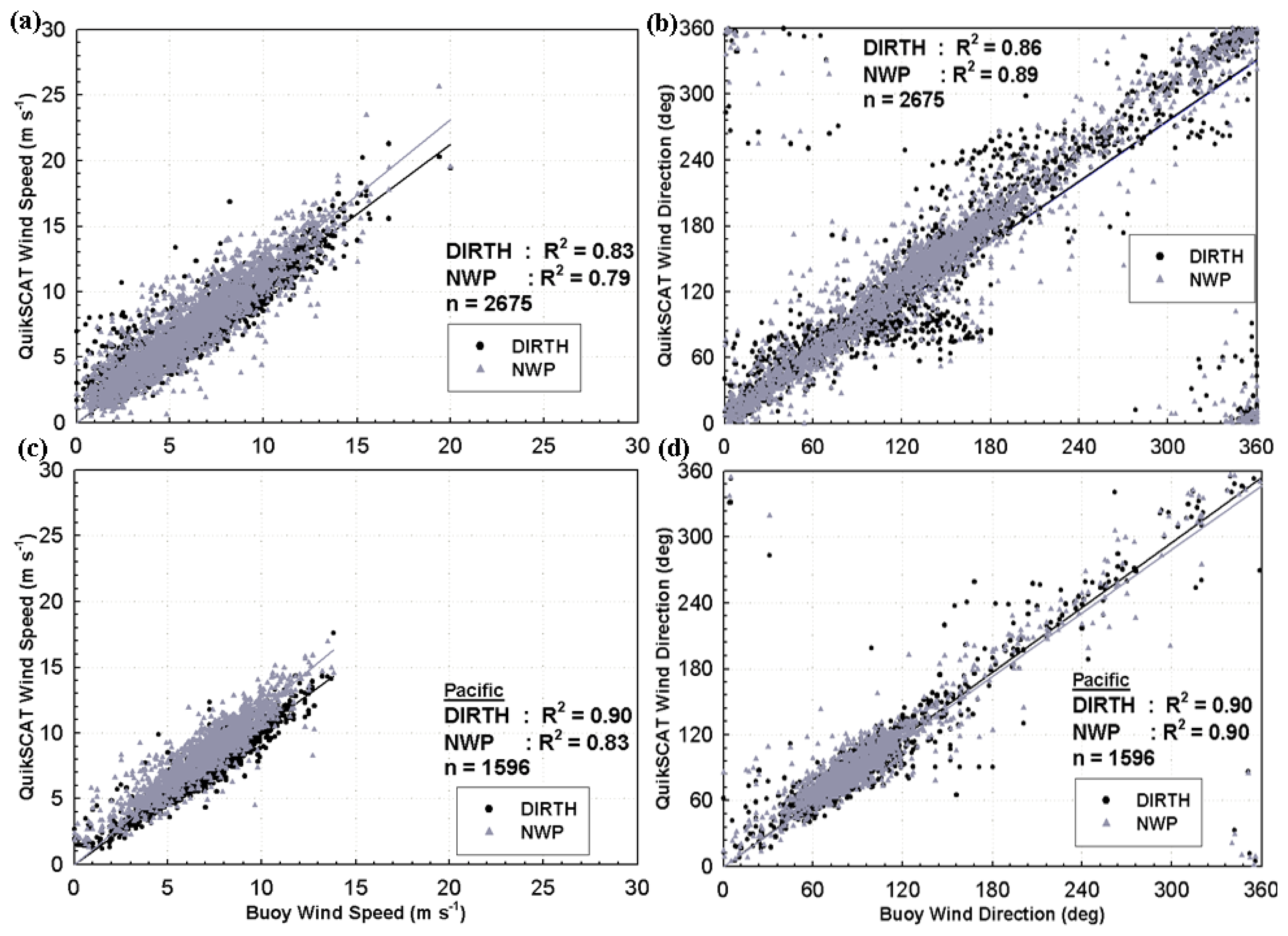
Wind data from QuikSCAT and the buoys are compared under various conditions to study the correlation trends. In making these comparisons we recognize that the buoy and satellite vector winds are measured at different temporal and spatial scales. For example, the scatterometer footprint is 12.5 or 25 km while the buoy measurements represent a local estimate and therefore include the wind variability on all scales (Stoffelen 1998). At first, all the data are compared directly with buoy data keeping a maximum time interval of 20 min and spatial interval of 0.1° (≈10 km) (Figure 3). Since QuikSCAT's performance at very light winds (< 3 m s-1) and strong winds (> 20 m s-1) are highly diminished (Freilich and Dunbar 1999; Ebuchi et al. 2002; Chao et al. 2003; Pickett et al. 2003), these conditions are also considered separately in assessing the regression coefficients (Figure 4). Comparisons of QuikSCAT wind at three offshore buoys located in the Pacific Ocean were also conducted as a comparison study with the GoM buoys due to reduced variability in the wind field and better performance of QuikSCAT at locations far from land. As noted earlier, the L2B product contains both the DIRTH and the NWP datasets with the NWP outputs approximately 100 m above the surface while DIRTH and buoys make measurements at 10 m neutral winds. Thus, in comparing NWP 100 m winds with QuikScat data, a mean difference is expected due to the climatological structure of the Planetary Boundary Layer (PBL). DIRTH shows slightly higher correlation than NWP for wind speed (R2=0.83 for DIRTH and R2 = 0.79 for NWP) (Figure 3a), while the wind direction correlations were about the same for both products (R2 = 0.86 for DIRTH and R2 = 0.89 for NWP) (Figure 3b). Overall, correlations were higher for wind speed and direction for the buoys located in the Pacific Ocean.
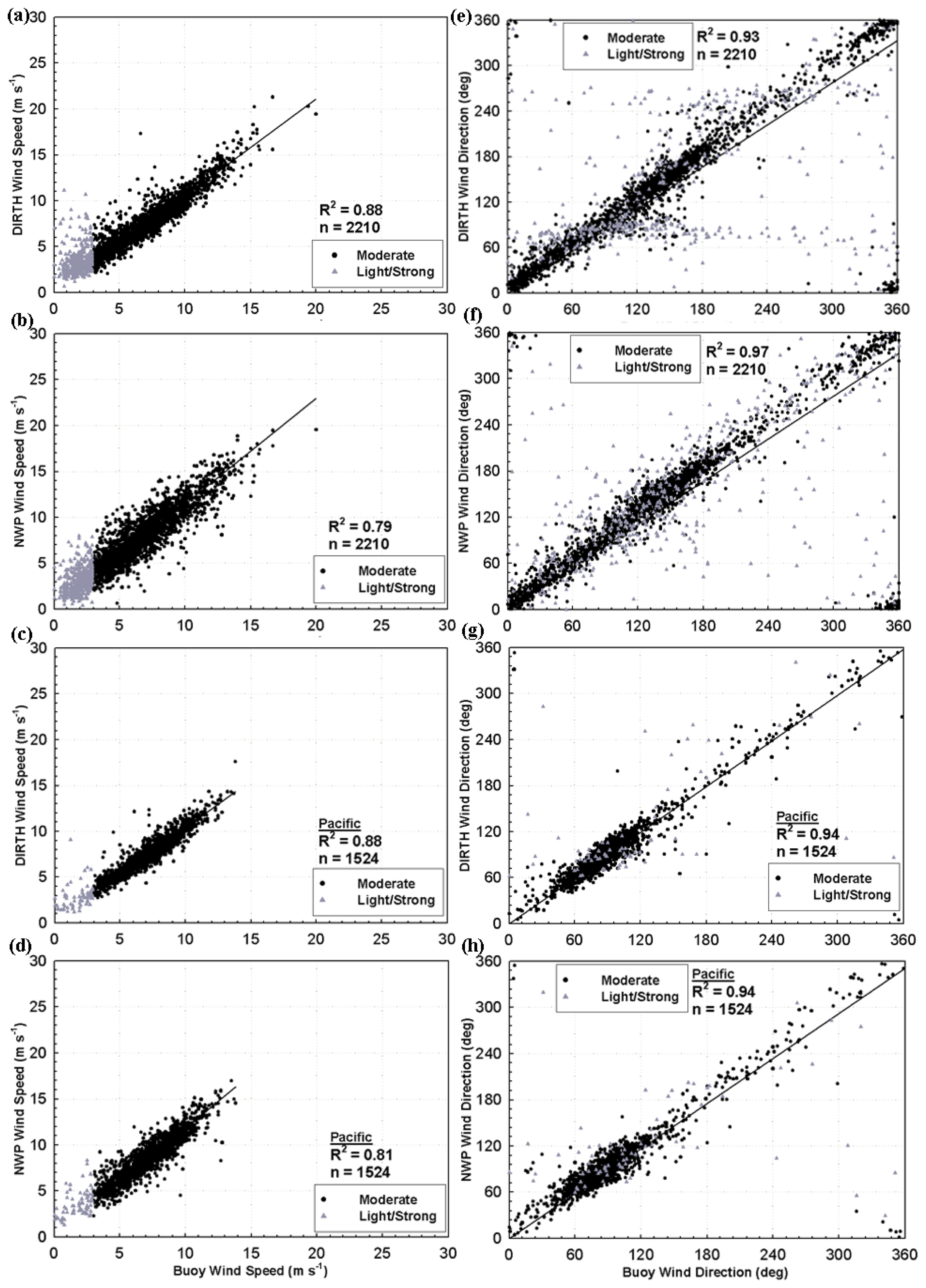
When only moderate winds are considered (i.e. speeds ranging from 3 to 20 m s-1) slightly higher R2 values are observed (Figure 4) suggesting minor adverse impact of light winds (gray color) on DIRTH measurements. Although DIRTH wind speed correlations were observed to be higher than NWP (Figure 4a, b), NWP correlation were higher than DIRTH for wind direction (Figure 4e, f). The Pacific Ocean dataset (Figure 4c, d, g, h) revealed about the same correlation compared to the GoM suggesting similar performance of QuikSCAT winds in the more open oceanic waters. It may be noted that DIRTH uses wind vector continuity as an ambiguity removal constraint that leads to rather smooth wind directions. Other methods that perform the ambiguity removal in a meteorologically balanced way have been presented (Portabella and Stoffelen 2004).
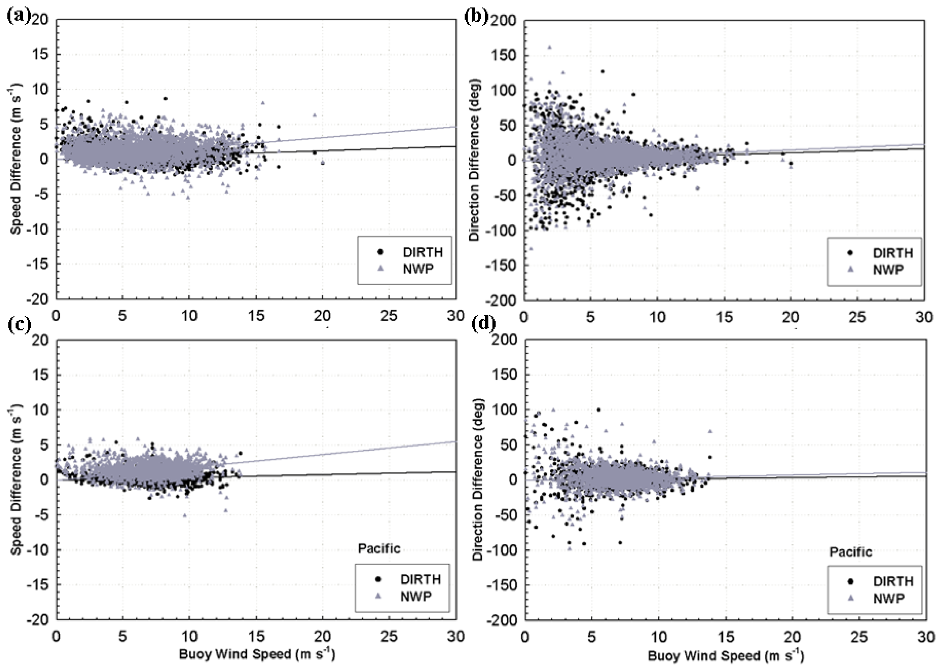
Differences in speed and direction between QuikSCAT L2B and buoy measurements plotted against buoy wind speed (Figure 5), provides an indication of QuikSCAT wind variability as a function of wind speed. The lines in the plots are regression lines and indicate the trend in the differences with respect to the zero line. A positive bias of QuikSCAT wind speeds in the Gulf of Mexico and the Pacific buoy locations (Figure 5a, c) are observed as expected for the NWP measurements.
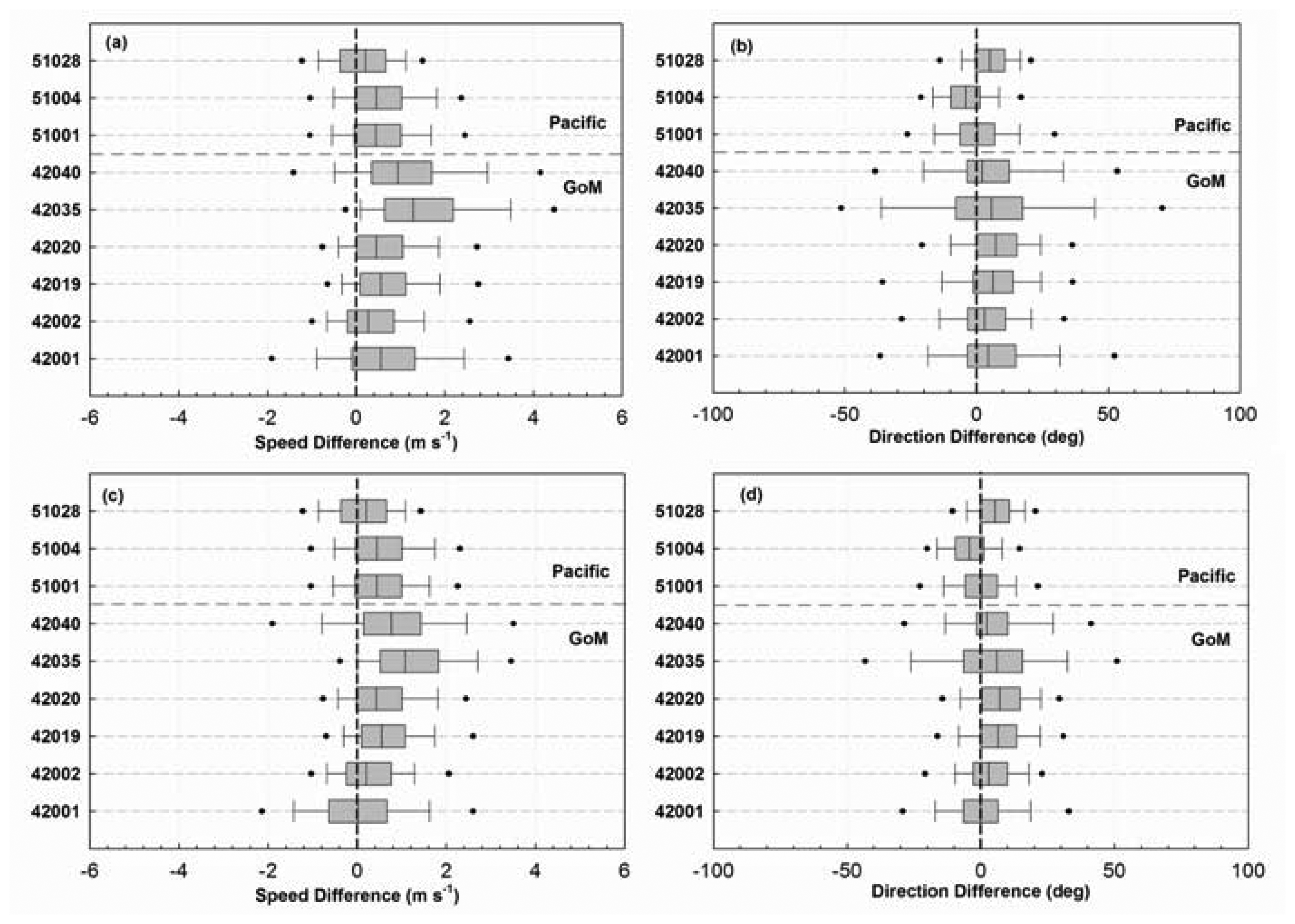
A positive bias is also observed for the NWP wind direction (Figure 5b, d). In comparison, the biases are much smaller for the DIRTH measurements. Overall we observe smaller biases in wind speed and direction for the Pacific Ocean buoys (Figure 5c, d). As documented in other studies (e.g., Stoffelen 1988; Tang et al. 2004) largest variations in wind direction are observed at light wind speeds with the accuracy of measurements increasing with increasing wind speeds. We also observed much greater scatter in the wind direction in the Gulf of Mexico buoys than in the Pacific Ocean. This was due to greater scatter of wind measurements at buoys located near the coast and also greater variability in wind speed and direction in the Gulf of Mexico (6.11±3.06 ms-1 and 142.8±87.8° for GoM versus 6.98 ± 2.27ms-1 and 96.4 ± 50.9° for the Pacific Ocean for the period 2005-07). Figure 6 provides an overview of the differences in speed and direction between QuikSCAT and each of the individual buoys considered in this study for i) DIRTH and NWP estimates, and ii) all wind data (Figure 6a, b) and moderate wind data (Figure 6c, d). The box plots of QuikSCAT and buoy differences (Figure 6) reveals overall better performance of the DIRTH wind speeds and direction than the NWP estimates. As indicated in Figure 5, NWP wind data exhibit greater biases than DIRTH measurements for all buoy locations. With most wind measurements being in the moderate range (3 to 20 m s-1), we observed only small differences in the variations when all wind data (Figure 6a, b) are compared to moderate winds (Figure 6c, d) for both the NWP and DIRTH data. In considering the performance of individual buoys, we observed least difference and biases for DIRTH measurements for the 3 Pacific Ocean buoys and the two offshore buoys (42001 and 42002) in the Gulf of Mexico. Buoys 42020 and 42019 which are about 100 and 127 km from the coast also show comparable differences to the offshore buoys in the Gulf of Mexico and the Pacific Ocean. However, they reveal greater positive biases in wind speed and direction measurements. The greatest differences and biases between QuikSCAT and buoy wind measurements are observed for the buoys 42040 and 42035 (Figure 1). Buoy 42035 is closest to the coast (54.7 km) and buoy 42040 is directly to the east of the Mississippi River delta. It is thus observed that QuikSCAT's performance is degraded due to land contamination and should thus be used with caution. Overall, this analysis indicates DIRTH wind speed and direction provides as expected better results than the NWP wind measurements.
2.2. Level 3 Gridded data
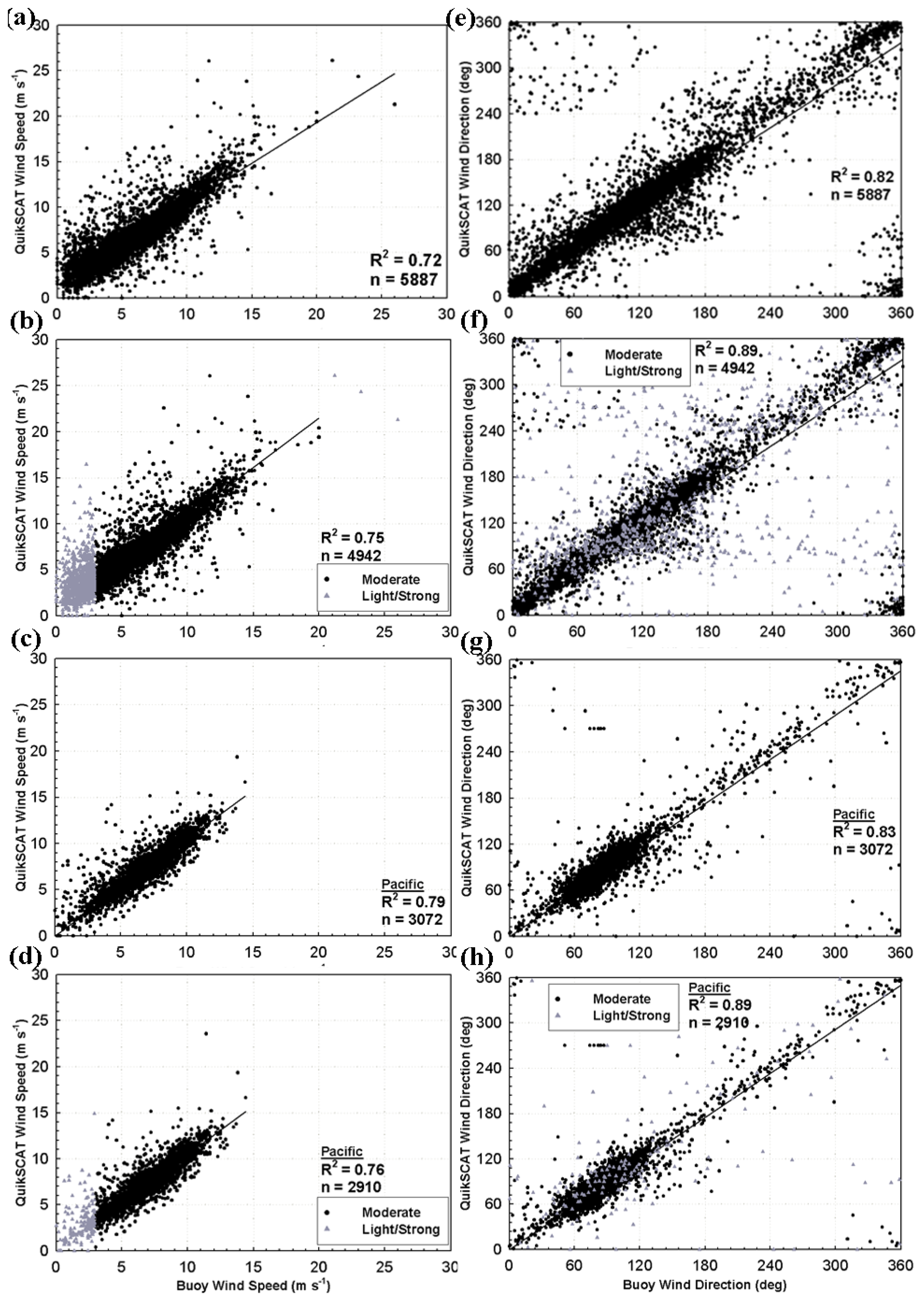
An analysis of L3 dataset also exhibited reasonably high coefficients of determination (R2) values for both wind speed and direction (Figure 7). For moderate winds, i.e. speeds ranging from 3 m s-1 to 20 m s-1, the correlation for the wind appears to increase slightly (from 0.72 to 0.75 for speed and 0.82 to 0.89 for direction). The adverse effect of light winds is thus noticeable. Both moderate and the light/strong winds (gray color) are shown for illustrating this point. Wind direction data points are observed to be more scattered for the light/strong winds. Pacific buoys showed small improvements over the GoM buoys. Light and strong winds do not appear to impact measurements in the open ocean too strongly. This may be due to lack of excess variation of wind speeds around the Pacific Ocean buoys during the study period.
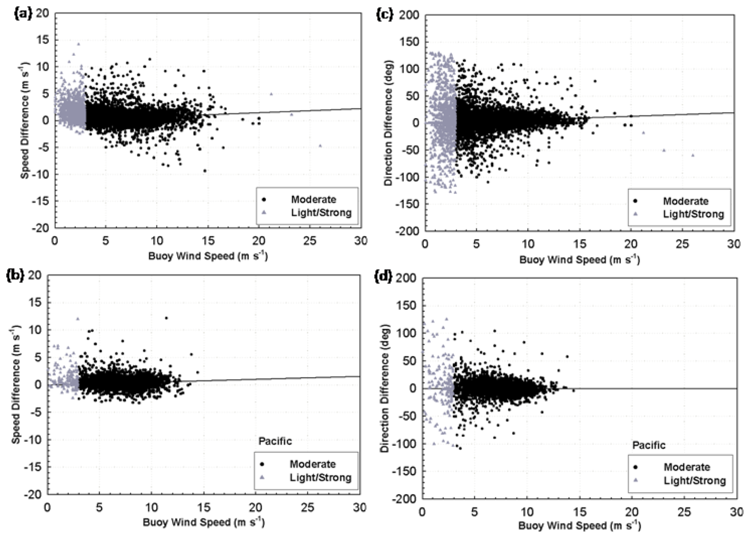
In Figure 8 the differences or residuals between QuikSCAT and buoy measurements (QuikSCAT – buoy) plotted against buoy wind speeds indicates the residual dependence on the buoy wind speed. There appears to be greater scatter in the wind speed differences for the GoM buoys than the Pacific buoys (Figure 8a, b). A general positive bias in the QuikSCAT wind measurements are observed with speed differences greater than 5 m s-1 for some wind data. For wind direction, the accuracy of measurements increased with wind speed with largest variations at light winds (Figure 8c, d). However, in comparison to the Pacific buoys, we observed greater scatter in the GoM buoys that could be attributed to reduced performance of QuikSCAT data near the coast. Box plots illustrating the performance of QuikSCAT at each buoy location are shown for speed and direction differences (Figure 9). In general, moderate L3 QuikSCAT wind data indicated smaller differences and less bias than when all wind data are considered (Figure 9a, b). Also in comparison to L2 DIRTH data, L3 wind data showed as expected greater positive bias for all the buoy locations including those in the Pacific. Buoys closer to land, however (e.g., 42035 and 42040) showed much higher differences compared to the relatively offshore buoys. These results describe the effect of land contamination on QuikSCAT measurements indicating that L3 wind measurements close to the coast must be used with caution.
Regression analysis were performed on the datasets to obtain the values of coefficient of determination (R2), RMSE, F-Test significance and two-sample t-test significance (Table 2). The F-test and t-test were performed to compare the QuikSCAT and buoy datasets for similarity in variance and means, respectively. The F-test was performed to determine if the differences in variances of the two datasets under consideration were significant and t-test was performed to determine if the difference in the means were significant. If the variances could be considered to be equal from the F-test, pooled t-test was performed assuming equal variances, else Satterwaithe t-test was performed assuming unequal variances. Results indicate that for wind speed the differences in the variances and means to be almost equal, while they are higher for wind direction. Correlation coefficients were found to be highest for the Level 2B - DIRTH wind speed while Level 2B - NWP showed the highest correlation for wind direction. RMSE errors for Level 2B and Level 3 GOM were observed to be in the same range as those determined for other oceanic regions (Ebuchi et al. 2002; Tang et al. 2004). Values of RMSE wind differences (satellite minus buoy) of 1.48 m s-1 and 29.5° for moderate L3 winds (Table 2) compared very closely to the 1.4 m s-1 and 37° obtained by Pickett et al. 2003 for nearshore buoy wind data off the U.S. West coast.
2.3. Hurricane Analysis
For the hurricane analysis, seven hurricanes and one tropical storm are considered (Table 3, tracks shown in Fig. 1) along with their dates of occurrence and their maximum intensity as reported by the best track analysis of the National Hurricane Center (NHC). The latest L2B (DIRTH) dataset has been observed to give a higher accuracy; hence, this dataset was used for this analysis. The maximum time difference between the measurements was maintained at 5 min and the maximum spatial difference at 0.1° (≈10 km). In all the cases, the results were encouraging (Figures 10 and 11). This indicates that QuikSCAT data follows the accuracy of buoy data closely during hurricanes. However, Hurricane Ivan appeared to be the only exception (Figure 10). As Hurricane Ivan traveled north, buoys 42003, 42040 and 42007 lay directly in its path. The time series (not shown) for these buoys were examined to see how the buoy wind measurements varied. Buoy 42003 measured a maximum wind speed of 28 m s-1 early on 15th September with the wind blowing towards west and then southwest. Buoy 42040 came closest to the eye of the hurricane and also measured a maximum wind speed of 28 m/s late on 15th September with the wind blowing towards the west. Just a few hours after this measurement, the buoy lost its mooring and went adrift due to the extreme turbulence and very high wave heights. Buoy 42007 measured a maximum wind speed of 26 m s-1 early on 16th September. It appeared that the unusually high wave heights (Stone et al. 2005; Wang et al. 2005) may have biased buoy measurements or eventually damaged the buoy structures.
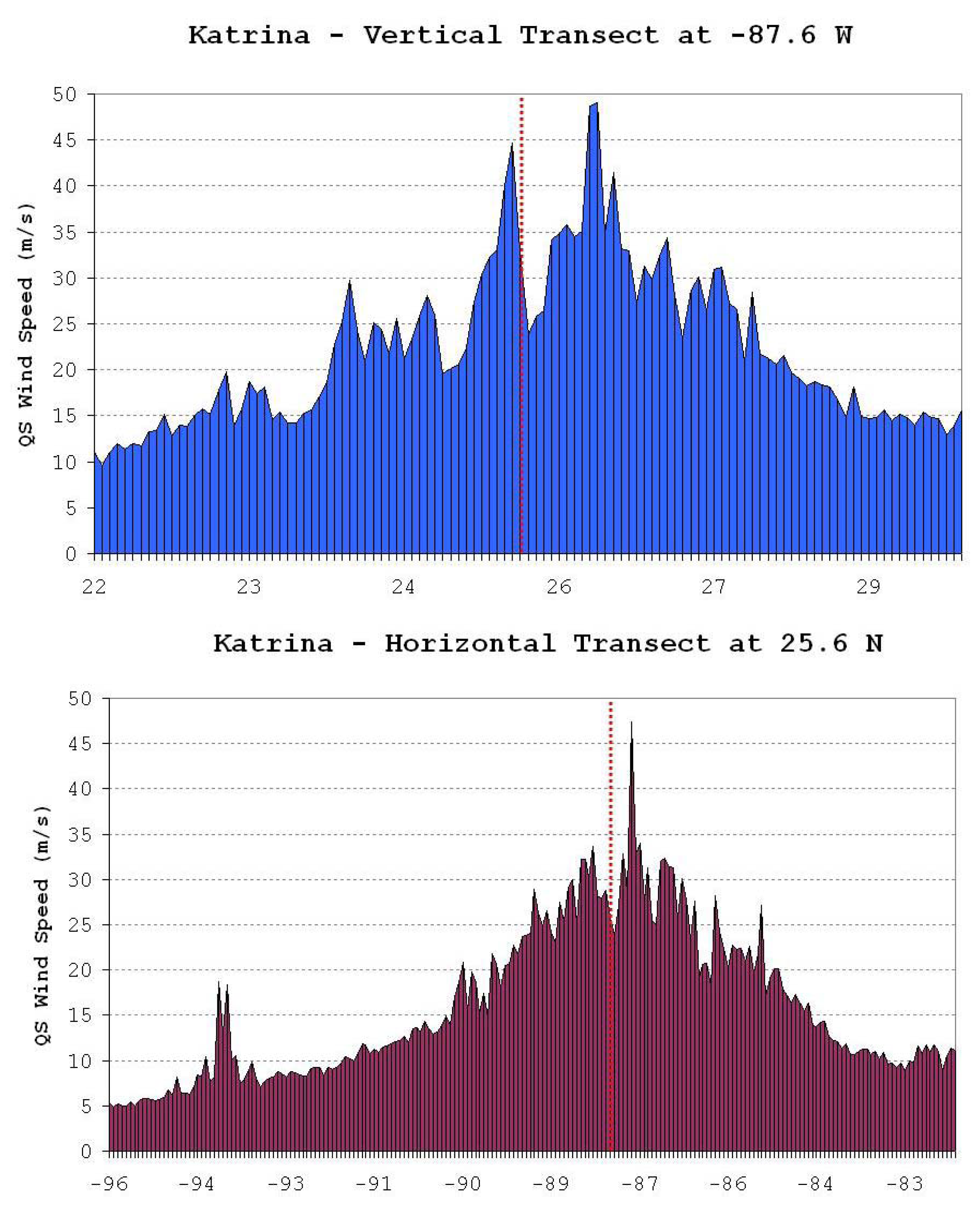
In the case of Hurricane Katrina, high correlations between QuikSCAT and buoy wind speed and direction measurements (Figure 11, second panel) were observed for speeds up to about 20 m s-1. High waves and wind sensor or buoy failure may have limited buoy wind measurements at much higher wind speeds. Buoy 42003 (Figure 1) for example stopped working at a maximum wind speed of 28.6 m s-1 on August 28, 2005. In Figure 12, L2B winds from QuikSCAT were plotted as wind vectors to create vector maps overlaid upon sea surface height anomaly (SSHA) measurements from Jason-1 for the Gulf of Mexico. The wind vectors were averaged and gridded along a 0.4° x 0.4° grid for clarity. A comparison of the vector maps of 27 and 28 August (Figure 12) indicated a noticeable increase in intensity of the hurricane as it travelled north across the Gulf of Mexico. Latitudinal and longitudinal transects across the eye of hurricane Katrina obtained on 28 August, 2005 revealed the extent of enhanced wind speeds and the radius of maximum wind (Figure 13). Maximum wind speeds of about 49 m s-1 were measured close to the eye of the hurricane. Although we observed a somewhat symmetric wind field about the eye of the hurricane with the greatest wind speeds to the west and north of the eye, due to rain contamination the generally very symmetric picture of the hurricane is often lost. This type of data should be useful for estimating the radius of maximum winds and critical wind radii that are generally obtained from aircraft reconnaissance.
3. Conclusions
Although, the regression analysis for the Level 3 (25 km) product resulted in fairly good correlations between QuikSCAT and buoys wind measurements, the Level 2B (12.5 km) product was clearly more accurate. The effect of light winds was quite apparent, thus the best results were observed for moderate winds. The accuracy of measurement, especially for wind direction, increased with wind speed. Reference Pacific buoys displayed expectedly good correlations; however, the regressions were only slightly better than those for the GoM buoys. This suggests that QuikSCAT was affected only by extreme proximity to land, as in the case of buoys 42035 and 42040, and the retrievals were fairly reliable in coastal regions. DIRTH displayed better regression for wind speed while NWP was better for wind direction. Since the NWP outputs are used for the wind direction ambiguity selection, these results indicate that either the ambiguity removal algorithm is not very efficient or the initial four solutions are inaccurate. The effect of land contamination is a major problem with QuikSCAT retrievals as the accuracy of measurement decreases with proximity to the coast.
The hurricane analysis results showed very good correlations between QuikSCAT Level 2B and buoys. Buoy data were however found to be limited in their reliability during extreme wind events. As the readings are averaged over 8-min intervals, the final wind measurement could be greatly diminished if the anemometer is blocked by high waves, or due to constant tipping of the buoy. Hence, despite their proximity to the hurricane, buoys tend to make much reduced measurements. QuikSCAT wind data have also been shown to be limited in their accuracy in the presence of excess rain. In addition, the geophysical model function (GMF) is also limited in its functionality, having a design limit of 30 m s-1, making it inherently inadequate for measuring hurricane-force winds. Hennon et al. (2006) evaluated the performance of the present GMFs (25 km and 12.5 km) provided by QuikSCAT and concluded that beyond 15 m s-1 QuikSCAT's wind retrieval accuracy are diminished. Yueh et al. (2003) conducted a study to correct for the attenuation and scattering caused by rain on QuikSCAT measurements using a parametric model developed for rain radars. Their results indicated very good correlations with NHC best track analysis when the rain model was incorporated in the measurements. This study however, has shown that the latest QuikSCAT L2 B DIRTH product can provide reasonably high wind observations with performance being shown to be comparable to buoys up to the limit of buoy measurements during storms and hurricanes.
Acknowledgments
This work has been supported by a NASA grant N06-4913 (Applied Sciences Program - Coastal Management) to E. J. D’Sa. The authors would like to acknowledge Drs. Larry Rouse, Mark Benfield and Nan Walker for their suggestions and Dr. Mitsuko Korobkin for the Jason-1 satellite processing. The authors are grateful to two reviewers for their comments and suggestions that helped improve this manuscript.
References and Notes
- Adams, I.S.; Jones, W.L.; Vasudevan, S.; Soisuvarn, S. Hurricane Wind Retrievals Using the SeaWinds Scatterometer on QuikSCAT. OCEANS Proceedings of MTS/IEEE 2005, 3, 2148–2150. [Google Scholar]
- Atlas, R.; Bloom, S.C.; Homan, R.N.; Brin, E.; Ardizzone, J.; Terry, J.; Bungato, D.; Jusem, J.C. Geophysical Validation of NSCAT Winds Using Atmosheric Data and Analyses. Journal of Geophysical Research 1999, 104(C5), 11405–11424. [Google Scholar]
- Brennan, M.J.; Knabb, R.D. Operational Evaluation of QuikSCAT Ocean Surface Vector Winds in Tropical Cyclones at the Tropical Prediction Center/National Hurricane Center, 10.5.
- Callahan, P.S. QuikSCAT Science Data Product User's Manual, Overview and Geophysical Data Products. V3.0. D-18053-RevA, JPL. 2006. ftp://podaac.jpl.nasa.gov/pub/ocean_wind/quikscat/doc/QSUG_v3.pdf.
- Chao, Y.; Li, Z.; Kindle, J.C.; Paduan, J.D.; Chavez, F.P. A High-Resolution Surface Vector Wind Product for Coastal Oceans: Blending Satellite Scatterometer Measurements with Regional Mesoscale Atmospheric Model Simulations. Geophysical Research Letters 2003, 30(1), 13.1–13.4. [Google Scholar]
- Chelton, D.B.; Schlax, M.G.; Freilich, M.H.; Milliff, R.F. Satellite Measurements Reveal Persistent Small-Scale Features in Ocean Winds. Science 2004, 303, 978–982. [Google Scholar]
- Chelton, D.B.; Freilich, M.H.; Sienkiewicz, J.M.; Von Ahn, J.M. On the Use of QuikSCAT Scatterometer Measurements of Surface Winds for Marine Weather Prediction. Monthly Weather Review 2006, 134, 2055–2070. [Google Scholar]
- Cione, J.J.; Uhlhorn, E.W. Sea Surface Temperature Variability in Hurricanes: Implications with Respect to Intensity Change. Monthly Weather Review 2003, 131, 1784–1796. [Google Scholar]
- Dunbar, R. S.; Perry, K.L. SeaWinds on QuikSCAT Level 3 Daily, Gridded Ocean Wind Vectors. JPL SeaWinds Project. 2001. Version 1.1, ftp://podaac.jpl.nasa.gov/pub/ocean_wind/quikscat/L3/doc/qscat_L3.pdf.
- Dunbar, R. S.; Hsiao, V.S.; Kim, Y.-J.; Pak, K.S.; Weiss, B.H.; Zhang, A. SeaWinds Algorithm Specifications. JPL D-21978. 2001. ftp://podaac.jpl.nasa.gov/ocean_wind/quikscat/doc/SWS_Algorithm_SpecsL1.pdf.
- Dunbar, R.S. Level 2B Data Software Interface Specification (SIS-2), SeaWinds Processing and Analysis Center, JPL. 2006. ftp://podaac.jpl.nasa.gov/pub/ocean_wind/quikscat/L2B/doc/L2B_SIS_200609.pdf.
- Ebuchi, N.; Graber, H.C.; Caruso, M.J. Evaluation of Wind Vectors Observed by QuikSCAT/SeaWinds Using Ocean Buoy Data. Journal of Atmospheric and Oceanic Technology 2002, 19, 2049–2061. [Google Scholar]
- Emanuel, K.A. Increasing Destructiveness of Tropical Cyclones over the Past 30 years. Nature 2005, 436, 686–688. [Google Scholar]
- Freilich, M.H.; Dunbar, R.S. The Accuracy of the NSCAT 1 Vector Winds: Comparisons with National Data Buoy Center Buoys. Journal of Geophysical Research 1999, 104(C5), 11231–11246. [Google Scholar]
- Freilich, M.H. SeaWinds Algorithm Theoretical Basis Document. NASA. ftp://podaac.jpl.nasa.gov/pub/ocean_wind/quikscat/doc/atbd-sws-01.pdf.
- Gilhousen, D.B. A field evaluation of NDBC moored buoy winds. Journal of Atmospheric and Oceanic Technology 1987, 4, 94–104. [Google Scholar]
- Hennon, C.C.; Long, D.G.; Wentz, F.J. Validation of QuikSCAT Wind Retrievals in Tropical Cyclone Environments, JP1.1. Joint Poster Session 1, Marine Meteorological Applications of Real and Synthetic Aperture Radar 2006. Joint between the 14th Conference on Interaction of the Sea and Atmosphere and 14th Conference on Satellite Meteorology and Oceanography. [Google Scholar]
- Hoffman, R.N.; Leidner, S.M. 2005. An introduction to the near-real-time QuikSCAT data. Weather and Forecasting 2005, 20, 476–493. [Google Scholar]
- Mears, C.; Smith, D.; Wentz, F. Detecting rain with QuikSCAT. Proceedings of the IEEE International Geoscience and Remote Sensing Symposium, Honolulu, Hawaii; 2002; 3, pp. 1235–1237. [Google Scholar]
- Pickett, M.H.; Tang, W.; Rosenfeld, L.K.; Wash, C.H. QuikSCAT Satellite Comparisons with Nearshore Buoy Wind Data off the U.S. West Coast. Journal of Atmospheric and Oceanic Technology 2003, 20, 1869–1878. [Google Scholar]
- Portabella, M.; Stoffelen, A. Rain detection and quality control of SeaWinds. Journal of Atmospheric and Oceanic Technology 2001, 18, 1171–1183. [Google Scholar]
- Portabella, M.; Stoffelen, A. A comparison of KNMI quality control and JPL rain flag for SeaWinds. Canadian Journal of Remote Sensing 2002, 28, 424–430. [Google Scholar]
- Ruti, P.M.; Marullo, S.; D’Ortenzio, S.; Tremant, M. Comparison of analyzed and measured wind speeds in the perspective of oceanic simulations over the Mediterranean basin: Analyses, QuikSCAT and buoy data. Journal of Marine Systems 2008, 70, 33–48. [Google Scholar]
- Shaffer, S.; Dunbar, R.S.; Hsiao, S.V.; Long, D.G. A median-filter-based ambiguity removal algorithm for NSCAT. IEEE Transactions on Geoscience and Remote Sensing 1991, 29, 167–174. [Google Scholar]
- Stiles, B.W. Special Wind Vector Data Product: Direction Interval Retrieval with Threshold Nudging (DIRTH), Product Description. Version 1.1. Jet Propulsion Laboratory. 1999. [Google Scholar]
- Stoffelen, A. Error modeling and calibration; towards the true surface wind speed. Journal of Geophysical Research 1998, 103(C4), 7755–7766. [Google Scholar]
- Stoffelen, A. A probabilistic approach for SeaWinds data assimilation. Quarterly Journal of Royal Meteorological Society 2004, 130, 127–152. [Google Scholar]
- Stone, G.W.; Walker, N.D.; Hsu, S.A.; Babin, A.; Liu, B.; Keim, B.D.; Teague, W.; Mitchell, D.; Leben, R. Hurricane Ivan's Impact Along The Northern Gulf of Mexico. EOS 2005, 86(48), 497–508. [Google Scholar]
- Tang, W.; Liu, W.T.; Stiles, B.W. Evaluation of High-Resolution Ocean Surface Vector Winds Measured by QuikSCAT Scatterometer in Coastal Regions. IEEE Transactions on Geoscience and Remote Sensing 2004, 42(8), 1762–1769. [Google Scholar]
- Wang, D.W.; Mitchell, D.A.; Teague, W.J.; Jarosz, E.; Hulbert, M.S. Extreme Waves Under Hurricane Ivan. Science 2005, 309, 896. [Google Scholar]
- Yueh, S.H.; Stiles, B.W.; Liu, W.T. QuikSCAT Wind Retrievals for Tropical Cyclones. IEEE Transactions on Geoscience and Remote Sensing 2003, 41(11), 2616–2627. [Google Scholar]
Figure 1.
Location of the buoys in the Gulf of Mexico along with tracks of all the hurricanes considered in this study.
Figure 1.
Location of the buoys in the Gulf of Mexico along with tracks of all the hurricanes considered in this study.
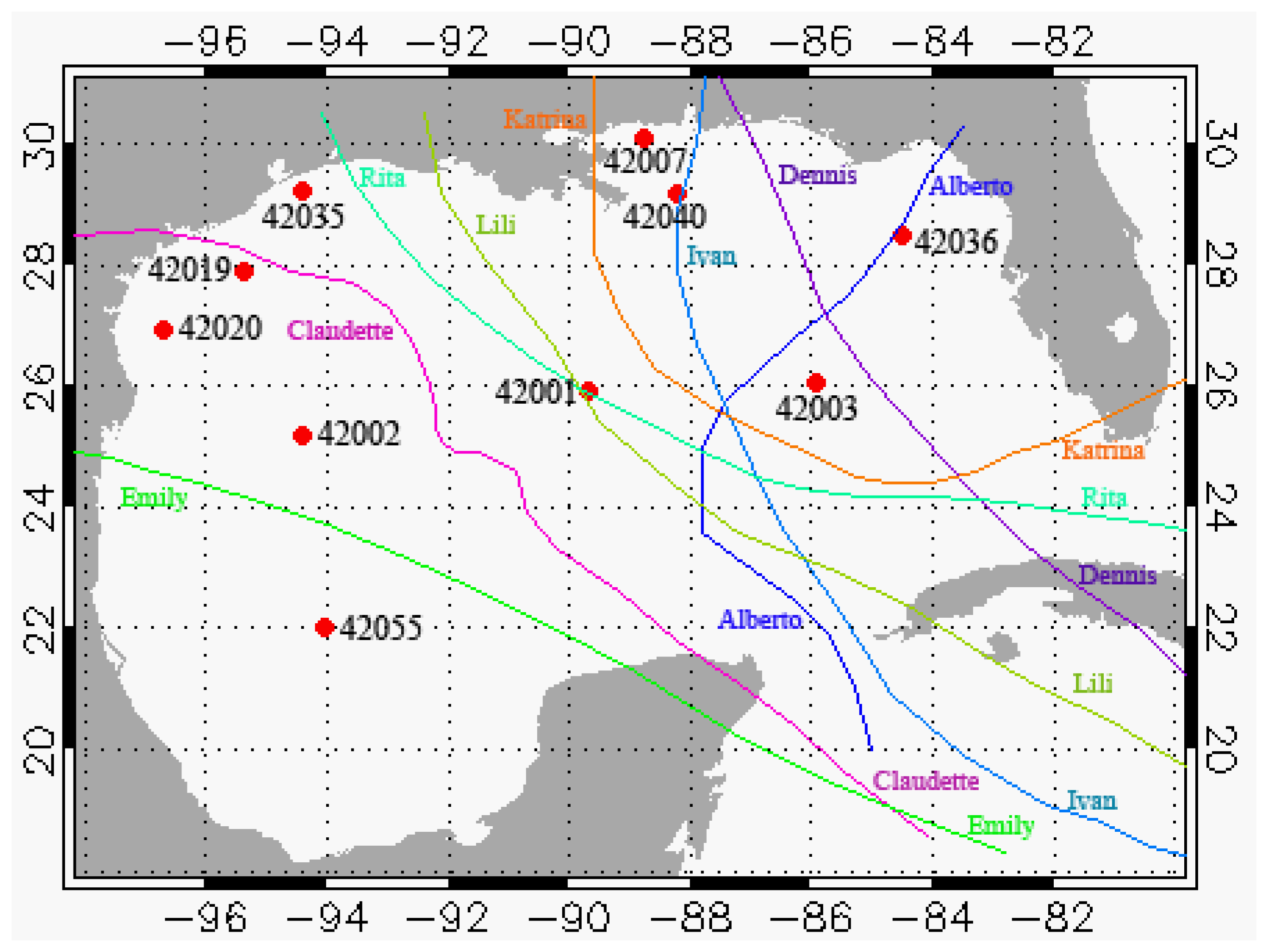
Figure 2.
Time Series of monthly averaged QuikSCAT wind speed for buoys 42001, 42002, 42019 and 42020 (blue line) is shown along with the difference in speed between QuikSCAT and buoy measurements (green line).
Figure 2.
Time Series of monthly averaged QuikSCAT wind speed for buoys 42001, 42002, 42019 and 42020 (blue line) is shown along with the difference in speed between QuikSCAT and buoy measurements (green line).
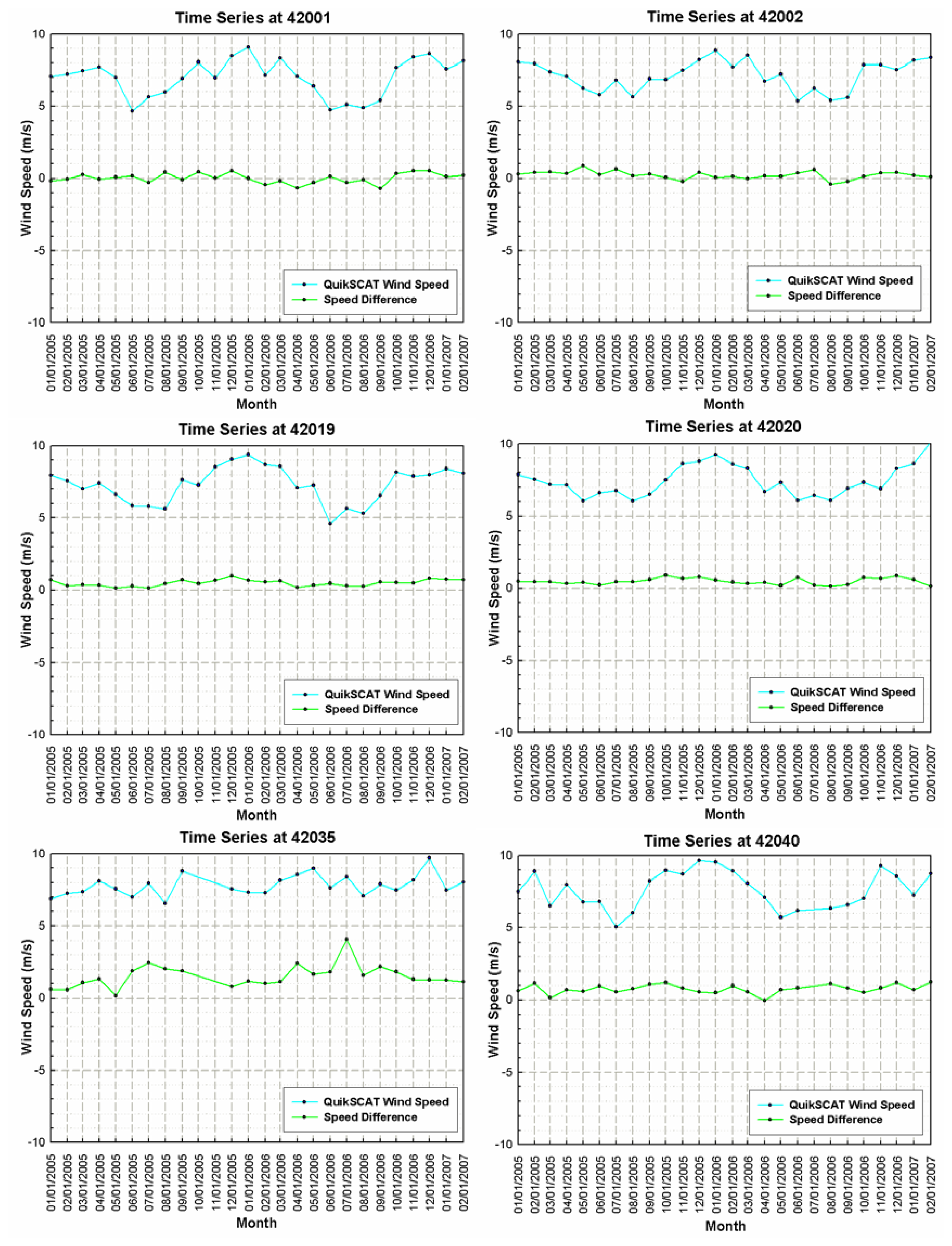
Figure 3.
Level 2B regressions for all wind speeds in the Gulf of Mexico (a, b) and the Pacific Ocean (c, d). Left panels depict wind speed measurements. Right panels depict wind direction measurements. ‘R2′ is the coefficient of determination and ‘n’ is the number of data points.
Figure 3.
Level 2B regressions for all wind speeds in the Gulf of Mexico (a, b) and the Pacific Ocean (c, d). Left panels depict wind speed measurements. Right panels depict wind direction measurements. ‘R2′ is the coefficient of determination and ‘n’ is the number of data points.

Figure 4.
Level 2B DIRTH regressions for moderate winds (light/strong winds in gray) in the Gulf of Mexico (a, b, e, f) and the Pacific Ocean (c, d, g, h). Left panels depict wind speed measurements. Right panels depict wind direction measurements. ‘R2′ is the coefficient of determination and ‘n’ is the number of data points for moderate winds only.

Figure 5.
Level 2B measurements shown as difference in QuikSCAT and buoy measurements in the Gulf of Mexico (a, b) and the Pacific Ocean (c, d). Left panels depict wind speed measurements. Right panels depict wind direction measurements.
Figure 5.
Level 2B measurements shown as difference in QuikSCAT and buoy measurements in the Gulf of Mexico (a, b) and the Pacific Ocean (c, d). Left panels depict wind speed measurements. Right panels depict wind direction measurements.

Figure 6.
Box plots depicting variations at individual buoys for speed (left panels) and direction (right panel) difference between QuikSCAT and buoys (x-axis). Top panels (a, b) show variations for all wind speeds. Bottom (c, d) panels show variations for moderate winds. The central lines of the boxes denote the median and the edges depict the 25th and 75th percentile. The error bars beyond the boxes depict the 10th and 90th percentile and the points depict the 5th and 95th percentile.
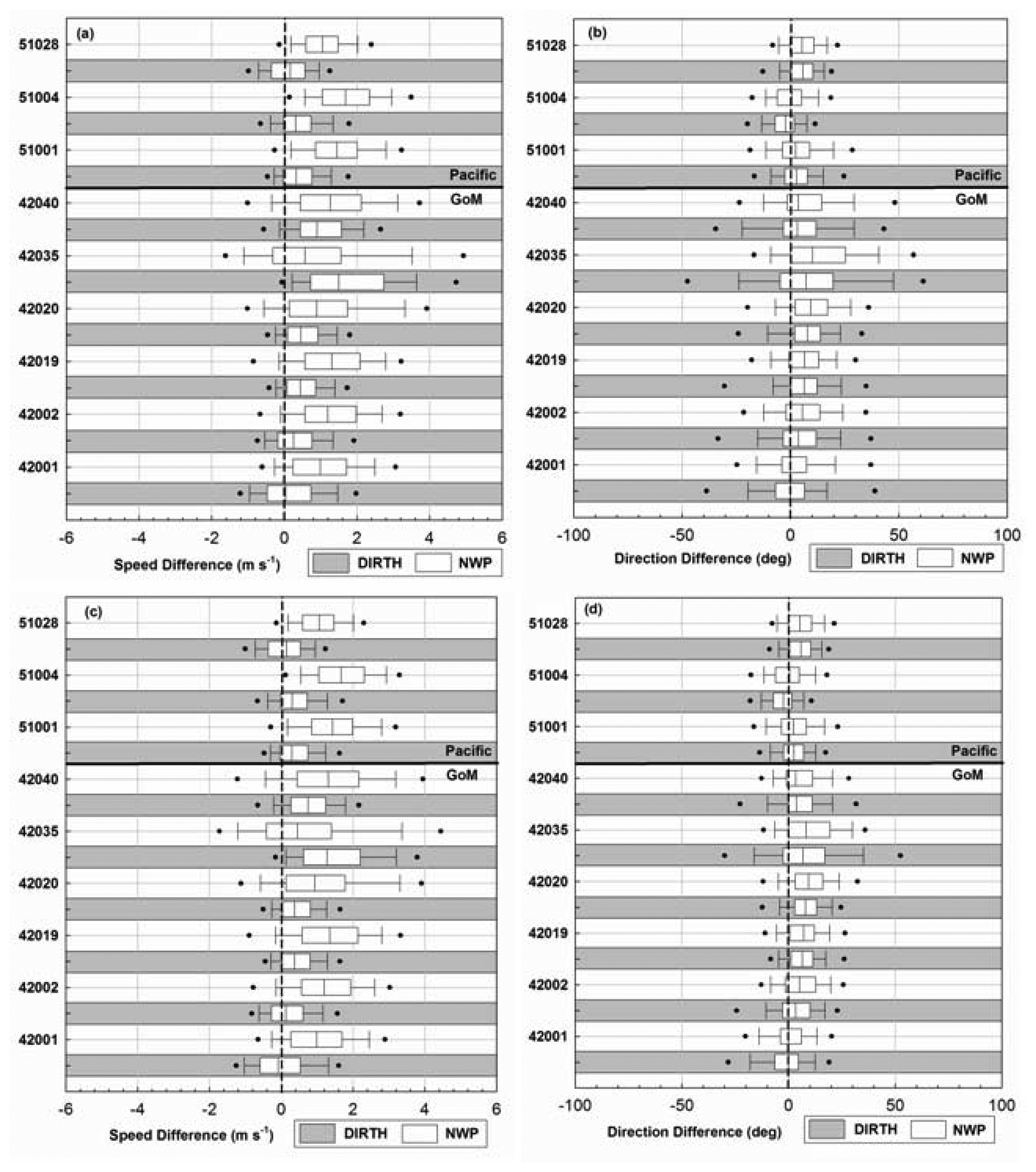
Figure 7.
Level 3 regressions in the Gulf of Mexico (a, b, e, f) and the Pacific Ocean (c, d, g, h). Left panels depict wind speed measurements and right panels depict wind direction measurements. ‘R2′ is the coefficient of determination and ‘n’ is the number of data points. Moderate winds are shown by dark symbols and light/strong winds are shown by gray symbols.

Figure 8.
Level 3 measurements shown as difference between QuikSCAT and buoy measurements for the Gulf of Mexico (a, c) and the Pacific Ocean (b, d) with dark symbols denoting moderate winds. Left panels depict wind speed measurements and right panels depict wind direction measurements. Line indicates the regression line.

Figure 9.
Box plots depicting variations at individual buoys for speed (left panels) and direction (right panel) difference between QuikSCAT and buoys. Top panels (a, b) show variations for all wind speeds. Bottom (c, d) panels show variations for moderate winds. The central lines of the boxes denote the median and the edges depict the 25th and 75th percentile. The error bars beyond the boxes depict the 10th and 90th percentile and the points depict the 5th and 95th percentile.

Figure 10.
Level 2B DIRTH regressions for hurricanes in the Gulf of Mexico. Left panels depict wind speed measurements. Right panels depict wind direction measurements.
Figure 10.
Level 2B DIRTH regressions for hurricanes in the Gulf of Mexico. Left panels depict wind speed measurements. Right panels depict wind direction measurements.
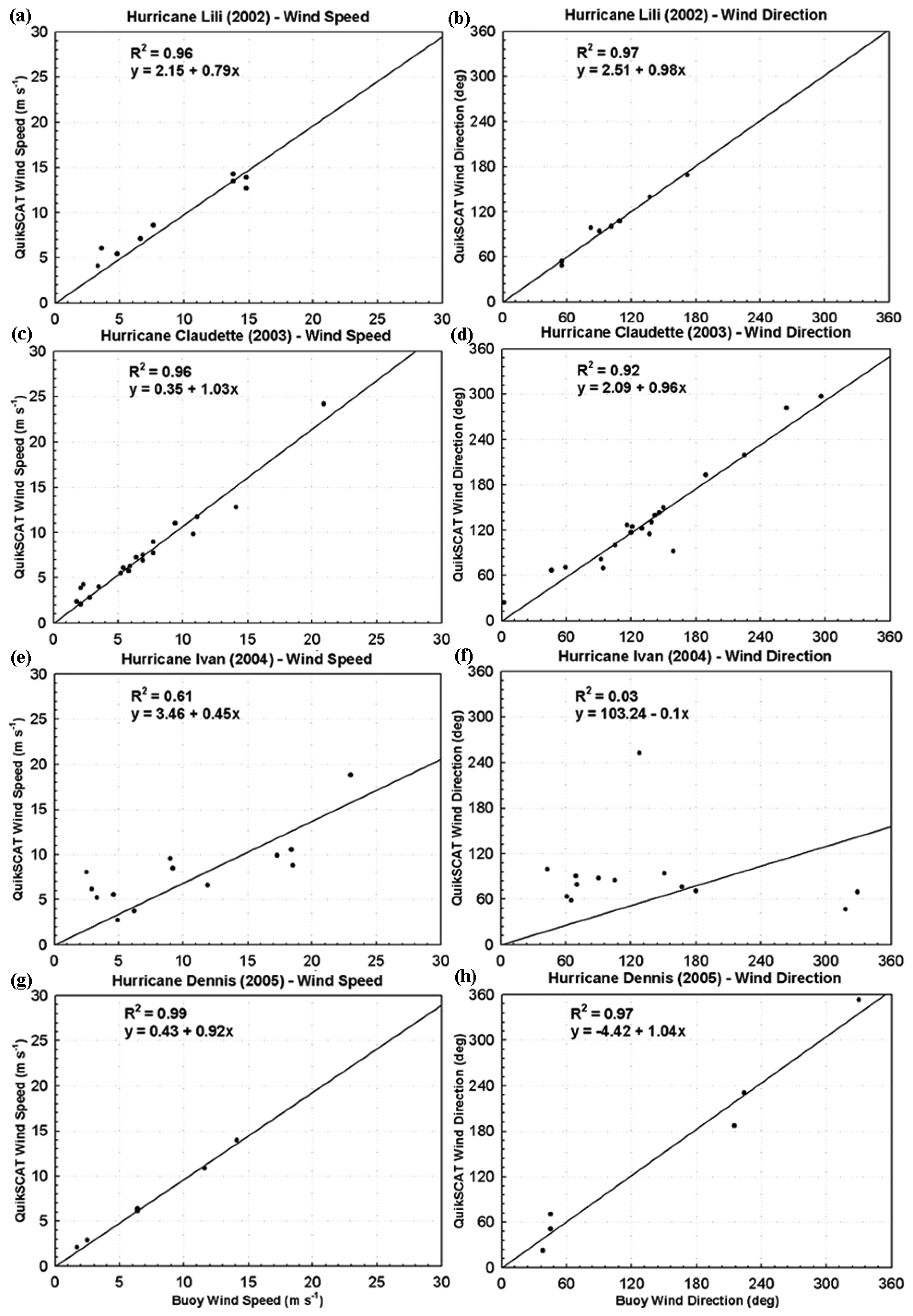
Figure 11.
Level 2B DIRTH regressions for hurricanes in the Gulf of Mexico. Left panels depict wind speed measurements. Right panels depict wind direction measurements.
Figure 11.
Level 2B DIRTH regressions for hurricanes in the Gulf of Mexico. Left panels depict wind speed measurements. Right panels depict wind direction measurements.
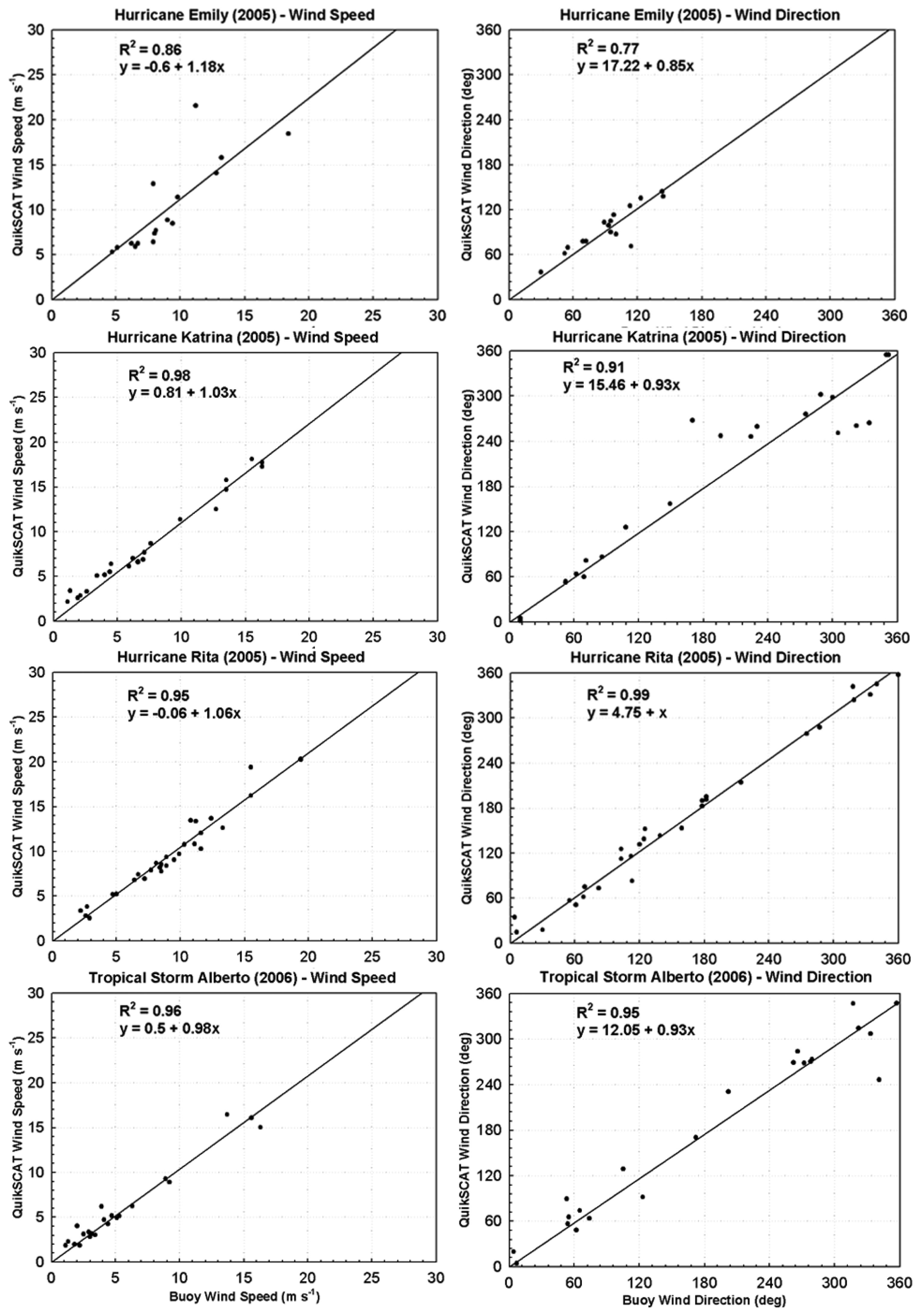
Figure 12.
Vector winds overlaid on top of Jason-1 satellite sea surface height anomaly (SSHA) map on 27th and 28th August 2005 during the passage of Hurricane Katrina.
Figure 12.
Vector winds overlaid on top of Jason-1 satellite sea surface height anomaly (SSHA) map on 27th and 28th August 2005 during the passage of Hurricane Katrina.
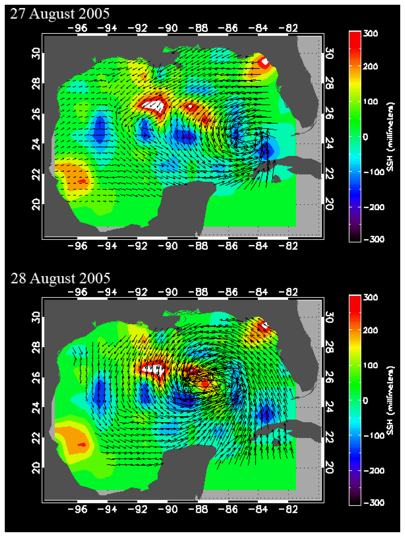
Figure 13.
Vertical (longitudinal) and horizontal (latitudinal) transects across the eye of the Hurricane Katrina on 28th August 2005 for the QuikSCAT L2B wind data. The red line depicts the location of the eye.
Figure 13.
Vertical (longitudinal) and horizontal (latitudinal) transects across the eye of the Hurricane Katrina on 28th August 2005 for the QuikSCAT L2B wind data. The red line depicts the location of the eye.

Table 1.
Buoy locations with mean and standard deviations for QuikSCAT measurements and difference between QuikSCAT and buoy measurements.
| Buoys | Distance from Coast (km) | Speed (m/s) | Direction (deg.) | Speed difference (m/s) | Direction difference (deg.) | ||||
|---|---|---|---|---|---|---|---|---|---|
| Mean | Std dev | Mean | Std dev | Mean | Std dev | Mean | Std dev | ||
| 42035 | 54.547 | 7.79 | 0.73 | 141.48 | 39.68 | 1.52 | 0.80 | 8.45 | 10.00 |
| 42040 | 87.94 | 7.61 | 1.30 | 155.08 | 52.52 | 0.76 | 0.32 | 3.91 | 7.47 |
| 42020 | 100.19 | 7.44 | 1.10 | 143.39 | 21.64 | 0.47 | 0.22 | 7.89 | 3.42 |
| 42019 | 127.13 | 7.29 | 1.24 | 144.31 | 25.08 | 0.48 | 0.23 | 6.52 | 5.37 |
| 42002 | 293.48 | 7.14 | 1.03 | 130.96 | 20.28 | 0.22 | 0.27 | 2.34 | 6.78 |
| 42001 | 364.88 | 6.98 | 1.29 | 135.91 | 31.51 | 0.008 | 0.34 | -1.76 | 6.31 |
Table 2.
Statistics for three QuikSCAT (QS) products in the Gulf of Mexico for wind speed and direction measurements in comparison to buoy measurements.
| Dataset | Speed | Direction | ||||||
|---|---|---|---|---|---|---|---|---|
| R2 | RMSE | F-test p-value | t-test p-value | R2 | RMSE | F-test p-value | t-test p-value | |
| QS Level 2B–DIRTH | ||||||||
| All Data | 0.83 | 1.24 | <0.0001 | <0.0001 | 0.86 | 33.77 | 0.6574 | 0.0493 |
| Moderate Winds (3-20 m s-1) | 0.88 | 0.94 | 0.0094 | <0.0001 | 0.93 | 23.31 | 0.7046 | 0.1408 |
| QS Level 2B – NWP | ||||||||
| All Data | 0.79 | 1.55 | 0.0008 | <0.0001 | 0.89 | 30.24 | 0.6840 | 0.0058 |
| Moderate Winds (3-20 m s-1) | 0.79 | 1.37 | <0.0001 | <0.0001 | 0.97 | 14.99 | 0.8860 | 0.0357 |
| QS Level 3 | ||||||||
| All Data | 0.72 | 1.69 | 0.0595 | <0.0001 | 0.82 | 40.52 | 0.5452 | 0.0001 |
| Moderate Winds (3-20 m s-1) | 0.75 | 1.48 | <0.0001 | <0.0001 | 0.89 | 29.53 | 0.7552 | 0.0028 |
Table 3.
Hurricane occurrence dates in the Gulf of Mexico and their maximum intensities according to the National Hurricane Center.
| Hurricane | Dates of Occurrence in GOM | Maximum Intensity – NHC | |
|---|---|---|---|
| m s-1 | knots | ||
| Lili | 2-3 October 2002 | 64.3 | 125 |
| Claudette | 12-15 July 2003 | 38.58 | 75 |
| Ivan | 14-15 September 2004 | 72.016 | 140 |
| Dennis | 5-7 July 2005 | 64.3 | 125 |
| Emily | 15-17 July 2005 | 72.016 | 140 |
| Katrina | 26-29 August 2005 | 77.16 | 150 |
| Rita | 20-25 September 2005 | 79.732 | 155 |
| Alberto (tropical storm) | 10-13 June 2006 | 30.864 | 60 |
© 2008 by MDPI Reproduction is permitted for noncommercial purposes.
Share and Cite
MDPI and ACS Style
Sharma, N.; D’Sa, E. Assessment and Analysis of QuikSCAT Vector Wind Products for the Gulf of Mexico: A Long-Term and Hurricane Analysis. Sensors 2008, 8, 1927-1949. https://doi.org/10.3390/s8031927
AMA Style
Sharma N, D’Sa E. Assessment and Analysis of QuikSCAT Vector Wind Products for the Gulf of Mexico: A Long-Term and Hurricane Analysis. Sensors. 2008; 8(3):1927-1949. https://doi.org/10.3390/s8031927
Chicago/Turabian StyleSharma, Neha, and Eurico D’Sa. 2008. "Assessment and Analysis of QuikSCAT Vector Wind Products for the Gulf of Mexico: A Long-Term and Hurricane Analysis" Sensors 8, no. 3: 1927-1949. https://doi.org/10.3390/s8031927