The Empirical Relationship between Mining Industry Development and Environmental Pollution in China

Abstract

This study uses a vector autoregression (VAR) model to analyze changes in pollutants among different mining industries and related policy in China from 2001 to 2014. The results show that: (1) because the pertinence of standards for mining waste water and waste gas emissions are not strong and because the maximum permissible discharge pollutant concentrations in these standards are too high, ammonia nitrogen and industrial sulfur dioxide discharges increased in most mining industries; (2) chemical oxygen demand was taken as an indicator of sewage treatment in environmental protection plans; hence, the chemical oxygen demand discharge decreased in all mining industries; (3) tax reduction policies, which are only implemented in coal mining and washing and extraction of petroleum and natural gas, decreased the industrial solid waste discharge in these two mining industries.

1. Introduction

Mineral resources are the material basis of economic development. In 2014, China’s oil production was 211.41 million tons, gas production was 124.81 billion cubic meters, and production of non-petroleum oils was 8.437 billion tons [1]. Mining promotes China’s economic development. In the past 10 years, the value of the mining industry has increased each year.

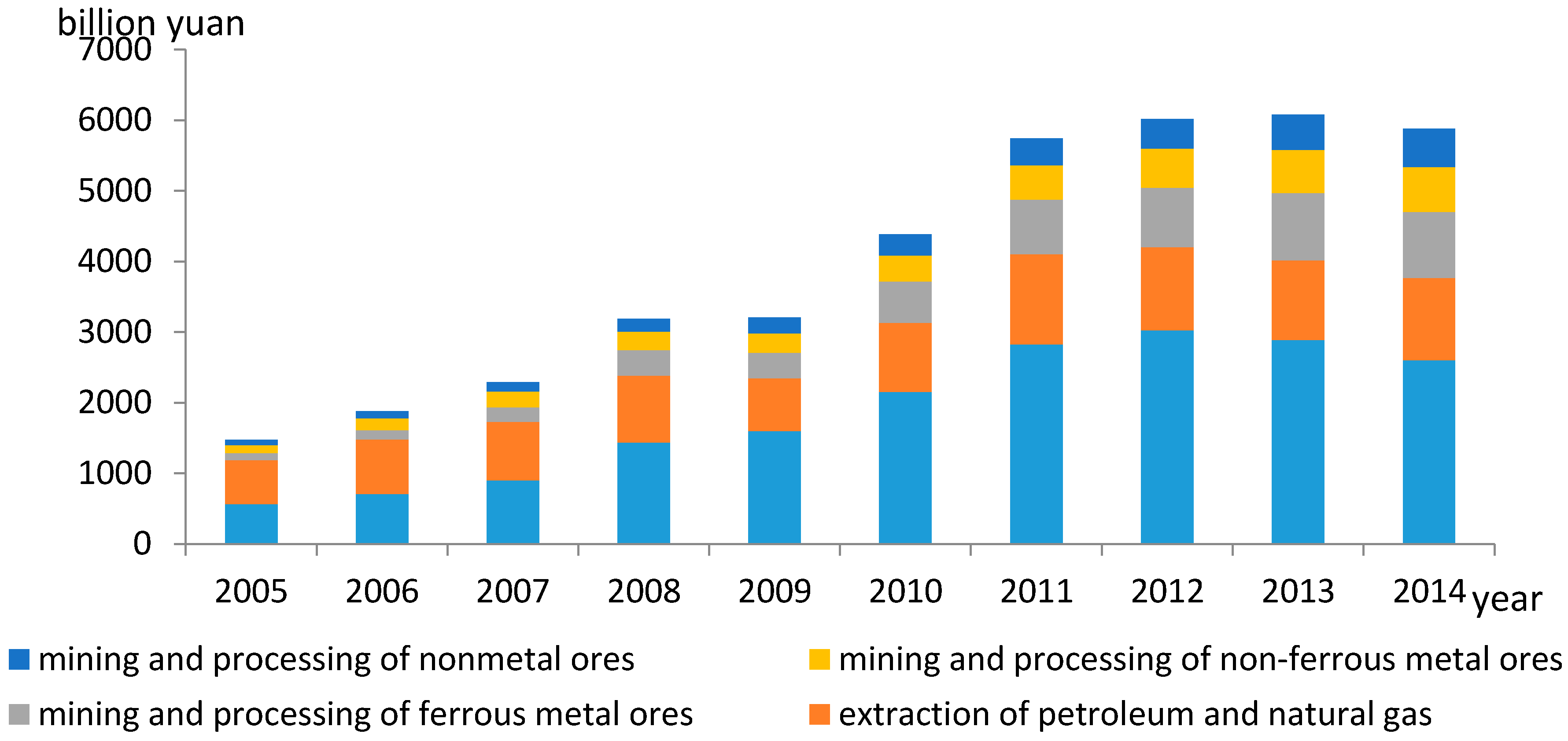
Except for in 2014, the mining industry added value accounted for more than 4% of the GDP [2,3,4,5,6,7,8,9,10,11,12,13,14,15,16,17,18,19,20,21,22,23,24,25,26,27,28,29]. In 2014, it was 58.788 trillion Yuan, nearly four times that in 2005 (Figure 1). Among the mining industries, coal mining and washing accounted for 44.27%, petroleum and natural gas extraction accounted for 19.84%, non-ferrous metal ore mining and processing accounted for 10.80%, ferrous metal ore mining and processing accounted for 15.87%, and non-metal ore mining and processing accounted for 9.22%. Furthermore, mining cities in which the mining industry is the dominant or pillar industry accounted for 34% of cities in China [30].

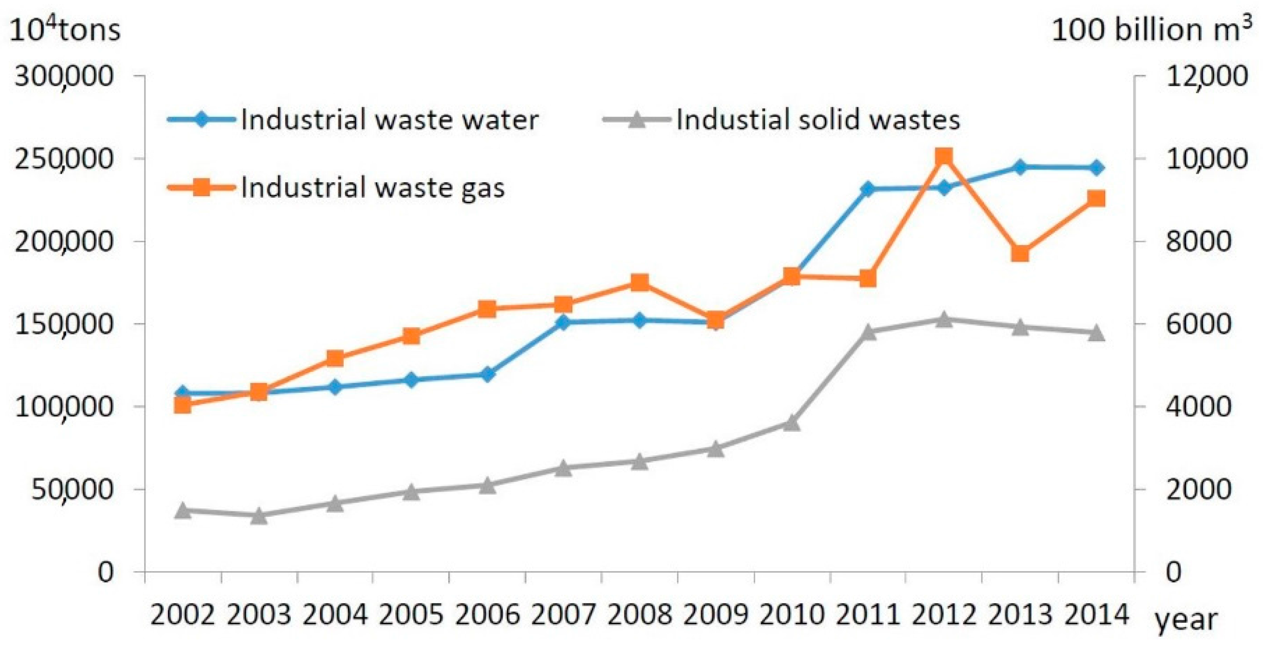
Mining activities cause great environmental disturbance. A variety of pollutants are generated in the process of ore mining. These pollutants diffuse into the surrounding environment and result in water, air and soil pollution problems. In 2014, 2531.67 million tons of industrial wastewater was discharged by the mining industry, nearly 2.2 times the 2005 amount; 903.6 billion cubic meters of industrial waste gas, nearly 1.3 times the 2005 amount; and 1449.32 million tons of industrial solid waste, nearly 3 times the 2005 amount (Figure 2). The chemical oxygen demand (COD) and ammonia nitrogen (AN) discharged in industrial wastewater were 1857.12 million and 74.31 million tons, respectively. The industrial sulfur dioxide (SO₂) discharged in industrial waste gas was 2192.59 million tons [31,32,33,34,35,36,37,38,39,40,41,42,43,44]. To control pollution from mining processes, 86,187.14 million Yuan were input for remediation of mine environments in 2014. Mining not only promotes economic development in China but also causes serious environmental pollution problems. The type and the degree of pollution vary depending on different mineral resources; hence, analysis of the nexus between industry development and environmental pollution for different mineral resources is important to compare their related environmental pollution problems and analyze the policies that cause the similarities and differences among them.

However, existing studies on the nexus between the mining industry and environmental pollution primarily focus on mine product consumption and energy minerals, including coal, oil and natural gas, which draw more attention due to the highlight on the greenhouse effect. Among them, the most studies are on coal consumption because it contributes more carbon per ton of oil equivalent than other resources such as oil and natural gas. These studies include Bloch et al. for China [45], Saboori and Sulaimanfor Malaysia [46], Tiwari et al. and Ahmad et al. for India [47,48] and Govindaraju and Tangfor India and China [49]. These studies all conclude that CO₂ emission is related to coal consumption. Compared with studies on coal consumption, there are fewer studies on oil and natural gas. Alkhathlan and Javid examined the relationship between oil and natural gas consumption and CO₂ emission in Saudi Arabia from 1980 to 2011, finding that they both lead to an increase in CO₂ emissions, and the CO₂ emissions can be reduced if the energy consumption structure switches from oil to natural gas [50]. Saboori and Sulaiman studied the relationship between natural gas and CO₂ emission. The results show that they have a positive relationship.

Although there are numerous studies on the environmental pollution resulting from mine product end consumption, studies on the environmental pollution caused by mine product production are few and focus on single minerals. Hence, it is impossible to contrast the differences in environmental pollution problems among different mineral resources or to discover the policies that cause them. For instance, Yu predicted China’s coal production environmental pollution in 2030, indicating that the turning point of the waste production per year will not occur until 2030 and the pollution caused by coal production will not increase to a great extent [51].

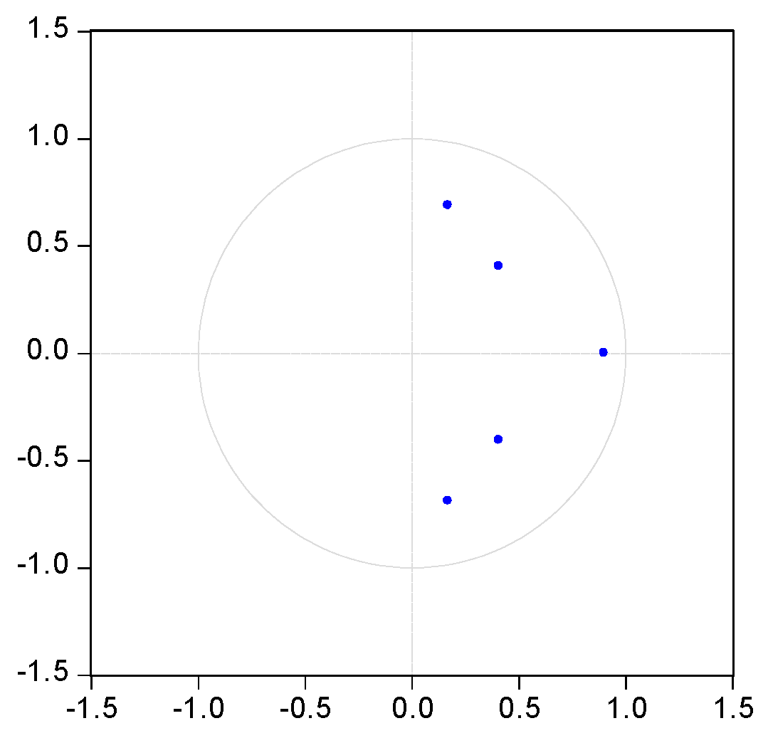
This paper uses the vector autoregression (VAR) model to analyze the water, air and solid pollution problems in coalmining and washing, petroleum and natural gas extraction, and non-ferrous metal ore, ferrous metal ore, and non-metal ore mining and processing. Through the establishment of the dynamic relationship between the gross industrial output value and the pollutant discharged in these five types of mining industries, the environmental pollution problems among them are compared and the policies that cause similarities and differences are analyzed. The VAR model has the following two characteristics. First, the estimation of traditional economic methods are based on economic theory and the theory cannot always rigorously describe the dynamic links among variables [52]. Compared with traditional econometric methods, the VAR model does not rely on these “incredible” economic assumptions. Second, the endogenous variables can appear on the right side of the equations well as be placed on the left side of the equation. This is complex for model to estimate and infer the relationship between variables [53]. Nevertheless, it is unnecessary to identify the endogenous and exogenous variables in the VAR model. Hence, it is used by many researchers [54,55,56] and is adopted in this paper to analyze the issue.

2. Econometric Methodology

2.1. VAR Model

The VAR model, proposed by Sims, is established based on the statistical properties of the data. It appears as the form of multiple simultaneous equations. In each equation, the dynamic relationship between all of the endogenous variable are estimated by the regression, which include the endogenous and the lagged value of endogenous. Moreover, it allows us to consider both long-and short-run restrictions justified by economic considerations [57]. The mathematical expression of the general VAR model is as follows:

$${\mathrm{y}}_{\mathrm{t}}=\mathrm{v}+{\mathrm{A}}_1{\mathrm{y}}_{\mathrm{t}-1}+\cdots +{\mathrm{A}}_{\mathrm{p}}{\mathrm{y}}_{\mathrm{t}-\mathrm{p}}+{\mathrm{B}}_0{\mathrm{x}}_{\mathrm{t}}+{\mathrm{B}}_1{\mathrm{x}}_{\mathrm{t}-1}+\cdots +{\mathrm{B}}_{\mathrm{q}}{\mathrm{x}}_{\mathrm{t}-\mathrm{q}}+{\mathrm{u}}_{\mathrm{t}}\mathrm{t}\in \left\{-\infty ,+\infty \right\}$$

(1)

where y_t, t = 1, T is a K × 1 time-series vector and A is a K × K parametric matrix. x_t is an M × 1 vector of exogenous variables and B is a K × M coefficient matrix to be estimated. u_t represents the random error term.

The large lag periods (p and q) makes it possible for the VAR model to reflect all of the dynamic innovations between variables. However, there is a shortage for the longer lag periods in which more parameters need to be estimated and there is a lower degree of freedom. Hence, it is necessary to make a reasonable choice between the lag periods and the freedom. The general principle is to adopt lag periods when the Swartz Criterion (SC) and Akaike Information Criterion (AIC) are the lowest. The formulas of these two statistics are expressed as follows:

$$\mathrm{AIC}=-2\mathrm{l}/\mathrm{n}+2\mathrm{k}/\mathrm{n}$$

(2)

$$\mathrm{SC}=-2\mathrm{l}/\mathrm{n}+\mathrm{k}\ln \mathrm{n}/\mathrm{n}$$

(3)

where k = m (qd + pm) represents the number of parameters to be estimated. n is the sample size and meets the following formula:

$$\mathrm{l}=-\mathrm{nm}\left(1+\ln 2\mathsf{\pi }\right)/2-\mathrm{n}\ln \left[\det \left({\displaystyle \sum }_{\mathrm{t}}{\widehat{\epsilon }}_t{\widehat{\epsilon }}_t^{\prime }/\mathrm{n}\right)\right]/2$$

(4)

2.2. Stationary Test

Most econometric models require a stable time series of variables. Hence, it is necessary to implement a stationary test before establishing the model for analysis. The unit root test is the standard method for checking if a sequence is stationary. The Augmented Dickey-Fuller (ADF), KPSS (Kwiatkowski Phillips Schmidt Shin) and Dickey-Fuller GLS (DFGLS) tests are three test methods. This paper uses the ADF test, which is the most widely used. Because a lagged difference term of the dependent variables is added into the regression equation, the ADF test can avoid the effects of higher-order serial correlation:

$$\Delta {\mathrm{y}}_{\mathrm{t}}={\mathsf{\eta }\mathrm{y}}_{\mathrm{t}-1}+{\displaystyle \sum }_{\mathrm{i}=\mathrm{i}}^{\mathrm{p}-1}{\mathsf{\beta }}_{\mathrm{i}}\Delta {\mathrm{y}}_{\mathrm{t}-\mathrm{i}}+{\mathrm{u}}_{\mathrm{t}}\mathrm{t}=1,2,\dots ,\mathrm{T}$$

(5)

$$\Delta {\mathrm{y}}_{\mathrm{t}}={\mathsf{\eta }\mathrm{y}}_{\mathrm{t}-1}+\mathsf{\alpha }+{\displaystyle \sum }_{\mathrm{i}=\mathrm{i}}^{\mathrm{p}-1}{\mathsf{\beta }}_{\mathrm{i}}\Delta {\mathrm{y}}_{\mathrm{t}-\mathrm{i}}+{\mathrm{u}}_{\mathrm{t}}\mathrm{t}=1,2,\dots ,\mathrm{T}$$

(6)

$$\Delta {\mathrm{y}}_{\mathrm{t}}={\mathsf{\eta }\mathrm{y}}_{\mathrm{t}-1}+\mathsf{\alpha }+\mathsf{\delta }\mathrm{t}+{\displaystyle \sum }_{\mathrm{i}=\mathrm{i}}^{\mathrm{p}-1}{\mathsf{\beta }}_{\mathrm{i}}\Delta {\mathrm{y}}_{\mathrm{t}-\mathrm{i}}+{\mathrm{u}}_{\mathrm{t}}\mathrm{t}=1,2,\dots ,\mathrm{T}$$

(7)

The following assumptions are then tested:

$${\mathrm{H}}_0:\mathsf{\eta }=0,{\mathrm{H}}_1:\mathsf{\eta }＜0$$

(8)

The original hypotheses is that the sequence of economic variable has a unit root, and the alternative hypothesis implies that the time series has no unit root. By testing whether the estimated value $\widehat{\mathsf{\eta }}$ rejects the null hypothesis, we can determine if the time series has a unit root.

2.3. Data Sources

We use annual time-series data from 2001 to 2014 for industrial output value, chemical oxygen demand discharged, ammonia nitrogen discharged, industrial SO₂ discharged and industrial solid wastes discharged in China. To avoid possible heteroscedasticity and multicollinearity problems, we transform all variables into logarithmic and differential form. Data on industrial output value represent the development of the mining industry and were obtained from the China Industry Economy Statistical Yearbook and the China Industry Statistical Yearbook. To eliminate the effect of price change, the industrial output value is calculated at a constant price (price-base year is 2000). The data for chemical oxygen demand discharged, ammonia nitrogen discharged, industrial SO₂ discharged and industrial solid wastes discharged represent the environmental pollution and were obtained from the China Statistical Yearbook on Environment. Among them, the chemical oxygen demand and ammonia nitrogen discharged are used as indicators of water pollution, industrial SO₂ discharged is used as an indicator of air pollution, and industrial solid waste is used as an indicator of solid pollution. The definitions of the variables are shown in

Table 1. Variables used in this study.

Variable	Definition	Units of Measure
GIOV	Gross industrial output value	yuan
COD	Chemical oxygen demand discharge	ton
AN	Ammonia nitrogen discharge	ton
ISW	Industrial solid waste	ton
SO2	Industrial sulfur dioxide emission	ton

.

3. Empirical Results

3.1. Results of the Unit-Root Tests

The results of the unit root test for all mining industries are presented in

Table 2. Unit root test results for coal mining and washing.

	Series	(I, T, K)	ADF	0.5 Critical Value	0.1 Critical Value	Prob. *
Levels	GIOV	(I, N, 0)	−2.843436	−3.119910	−2.701103 *	0.0793
	COD	(I, T, 1)	−5.610523	−3.875302 **	−3.388330 *	0.0044
	AN	(N, N, 0)	1.014372	−1.970978	−1.603693	0.9077
	ISW	(N, N, 0)	−1.078925	−1.970978	−1.603693	0.2388
	SO2	(I, T, 0)	−4.639636	−3.828975 **	−3.362984 *	0.0146
First difference	GIOV	(I, N, 0)	−7.240146	−3.175352 **	−2.728985 *	0.0001
	COD	(I, N, 0)	−2.945721	−3.144920	−2.713751 *	0.0691
	AN	(I, N, 0)	−4.119500	−3.144920 **	−2.713751 *	0.0100
	ISW	(N, N, 0)	−1.948815	−1.974028	−1.602922 *	0.0525
	SO2	(I, N, 1)	−4.903284	−3.175352 **	−2.728985 *	0.0035

Note: (I, T, K): I is the intercept, T is the trend, L is the lag length, and N is none; * and ** denote the null hypothesis of a unit root rejected at the 10% and 5% significance levels, respectively.

,

Table 3. Unit root test results for petroleum and natural gas extraction.

	Series	(I, T, K)	ADF	0.5 Critical Value	0.1 Critical Value	Prob. *
Levels	GIOV	(N, N, 0)	2.342212	−1.970978	−1.603693	0.9911
	COD	(I, T, 0)	−3.633524	−3.828975	−3.362984 *	0.0671
	AN	(I, N, 0)	−1.353440	−1.970978	−1.603693	0.1546
	ISW	(I, T, 0)	−4.426978	−3.828975	−3.362984	0.0201
	SO2	(N, N, 0)	−0.762549	−1.970978	−1.603693	0.3663
First difference	GIOV	(I, N, 0)	−2.917358	−3.144920	−2.713751 *	0.0848
	COD	(I, N, 1)	−4.322892	−3.175352 **	−2.728985 *	0.0083
	AN	(I, N, 0)	−3.971944	−3.144920 **	−2.713751 *	0.0128
	ISW	(I, N, 0)	−8.541855	−3.144920 **	−2.713751 *	0.0000
	SO2	(I, N, 0)	−3.152109	−3.144920 **	−2.713751 *	0.0494

Note: (I, T, K): I is the intercept, T is the trend, L is the lag length, and N is none; * and ** denote the null hypothesis of a unit root rejected at the 10% and 5% significance levels, respectively.

,

Table 4. Unit root test results for non-ferrous metal ore mining and processing.

	Series	(I, T, K)	ADF	0.5 Critical Value	0.1 Critical Value	Prob. *
Levels	GIOV	(N, N, 2)	1.293183	−1.977738	−1.602074	0.9387
	COD	(N, N, 0)	0.593911	−1.970978	−1.603693	0.8312
	AN	(I, T, 0)	−2.941565	−3.119910	−2.701103 *	0.0674
	ISW	(N, N, 0)	0.457459	−1.970978	−1.603693	0.7987
	SO2	(N, N, 0)	−0.775078	−1.970978	−0.1603683	0.3608
First difference	GIOV	(I, T, 1)	−3.737389	−3.933364	−3.420030 *	0.0653
	COD	(I, N, 0)	−3.441553	−3.144920 **	−2.713751 *	0.0308
	AN	(I, N, 0)	−6.981994	−3.144920 **	−2.713751 *	0.0001
	ISW	(I, N, 0)	−4.756370	−3.144920 **	−2.713751 *	0.0036
	SO2	(I, N, 0)	−3.335679	−3.144920 **	−2.713751 *	0.0366

Note: (I, T, K): I is the intercept, T is the trend, L is the lag length, and N is none; * and ** denote the null hypothesis of a unit root rejected at the 10% and 5% significance levels, respectively.

,

Table 5. Unit root test results for ferrous metal ore mining and processing.

	Series	(I, T, K)	ADF	0.5 Critical Value	0.1 Critical Value	Prob. *
Levels	GIOV	(I, N, 1)	−3.317284	−3.144920 **	−2.713751 *	0.0377
	COD	(I, T, 2)	−3.783048	−3.933364	−3.420030 *	0.0616
	AN	(I, N, 0)	−2.945174	−3.119910	−2.701102 *	0.0670
	ISW	(N, N, 0)	0.180184	−1.970973	−1.603693	0.7222
	SO2	(N, N, 0)	−0.838323	−1.970978	−1.603693	0.3334
First difference	GIOV	(I, T, 1)	−5.608179	−3.933364 **	−3.420030 *	0.0055
	COD	(I, N, 0)	−2.720846	−3.144920	−2.713751 *	0.0989
	AN	(I, N, 0)	−4.190148	−3.144920 **	−2.713751 *	0.0090
	ISW	(I, N, 1)	−3.874464	−3.175352 **	−2.728985 *	0.0166
	SO2	(I, N, 0)	−3.310650	−3.144920 **	−2.713751 *	0.0381

Note: (I, T, K): I is the intercept, T is the trend, L is the lag length, and N is none; * and ** denote the null hypothesis of a unit root rejected at the 10% and 5% significance levels, respectively.

and

Table 6. Unit root test results for non-metal ore mining and processing.

	Series	(I, T, K)	ADF	0.5 Critical Value	0.1 Critical Value	Prob.*
Levels	GIOV	(N, N, 1)	0.664558	−1.974028	−1.602922	0.8452
	COD	(N, N, 2)	−0.934667	−1.977738	−1.602074	0.2901
	AN	(I, N, 0)	−5.096009	−3.119910 **	−2.701103 *	0.0018
	ISW	(N, N, 0)	0.600191	−1.970978	−1.603693	0.8326
	SO2	(N, N, 0)	−0.704130	−1.970978	−1.603693	0.3920
First difference	GIOV	(I, N, 0)	−2.894985	−3.175352	−2.728985 *	0.0774
	COD	(I, N, 1)	−4.635565	−3.175352 **	−2.728985 *	0.0052
	AN	(I, N, 1)	−5.388098	−3.175352 **	−2.728985 *	0.0017
	ISW	(I, N, 0)	−3.075061	−3.144920	−2.713751 *	0.0560
	SO2	(I, N, 0)	−3.137956	−3.144920	−2.713751 *	0.0506

Note: (I, T, K): I is the intercept, T is the trend, L is the lag length, and N is none; * and ** denote the null hypothesis of a unit root rejected at the 10% and 5% significance levels, respectively.

. The results show that the null hypotheses of a unit root are not rejected in all variables but are rejected in their first-order difference at a 10% significance level.

Thus, the variables are not all a stationary sequence, but their first-order difference is a stationary sequence. Thus, the co-integration tests can be conducted.

3.2. Johansen Co-Integration Tests

Because most time series of economic variables are non-stationary, a differencing method is often used in building a reasonable VAR model to eliminate the non-stationary trend. However, the variables in the first-order difference equation often do not have direct economic significance. To solve this problem, Engle and Granger proposed the co-integration theory and methods to build a reasonable mode for non-stationary series [58]. The theory suggests that some linear combination of economic variables may be stationary, even though the variables are not stationary and call this stationary linear combination a co-integration equation.

The Johansen co-integration is a widely used multivariate con-integration method and it is based on the VAR model. In this paper, the trace statistic is used to determine whether there is a co-integration relationship. The results of the Johansen co-integration tests between the logarithm of gross of industrial output value (LGIOV), logarithm of chemical oxygen demand (LCOD), logarithm of ammonia nitrogen (LAN), logarithm of industrial SO₂ (LSO₂) and logarithm of industrial solid wastes (LISW) of all mining industries are presented in

Table 7. Johansen co-integration test for coal mining and washing.

	Hypothesized No. of CE(s)	Eigen Value	Trace Statistic	0.1 Critical Value	Prob. **
AN	None *	0.575470	15.54843	13.42878	0.0491
	At most 1 *	0.355274	5.267164	2.705545	0.0217
COD	None *	0.9222961	36.11994	13.42878	0.0000
	At most 1 *	0.360168	5.358602	2.705545	0.0206
ISW	None *	0.613525	16.00155	13.42878	0.0419
	At most 1 *	0.318033	4.593290	2.705545	0.0321
SO2	None *	0.602425	14.56814	13.42878	0.0686
	At most 1 *	0.252962	3.499675	2.705545	0.0614

Note: * denotes the null hypothesis rejected at a 10% significance level; ** denotes the null hypothesis rejected at a 5% significance level.

,

Table 8. Johansen co-integration test for petroleum and natural gas extraction.

	Hypothesized No. of CE(s)	Eigen Value	Trace Statistic	0.1 Critical Value	Prob. **
AN	None *	0.647262	14.29508	10.47457	0.0231
	At most 1 *	0.138627	1.790728	2.976163	0.2127
COD	None *	0.578479	10.48204	10.47457	0.0997
	At most 1 *	0.009571	0.115407	2.976163	0.7797
ISW	None *	0.490082	10.75556	10.47457	0.0902
	At most 1 *	0.199717	2.673485	2.976163	0.1206
SO2	None *	0.602425	14.56814	13.42878	0.0686
	At most 1 *	0.252962	3.499675	2.705545	0.0614

Note: * denotes the null hypothesis rejected at a 10% significance level; ** denotes the null hypothesis rejected at a 5% significance level.

,

Table 9. Johansen co-integration test for non-ferrous metal ore mining and processing.

	Hypothesized No. of CE(s)	Eigen Value	Trace Statistic	0.1 Critical Value	Prob. **
AN	None *	0.684011	18.74787	13.42878	0.0156
	At most 1 *	0.336531	4.923283	2.705545	0.0265
COD	None *	0.900634	31.84773	13.42878	0.0001
	At most 1 *	0.291803	4.140395	2.705545	0.0419
ISW	None *	0.649359	16.83893	13.42878	0.0312
	At most 1 *	0.299003	4.263022	2.705545	0.0389
SO2	None *	0.665964	17.64016	13.42878	0.0234
	At most 1 *	0.311704	4.482436	2.705545	0.0342

Note: * denotes the null hypothesis rejected at a 10% significance level; ** denotes the null hypothesis rejected at a 5% significance level.

,

Table 10. Johansen co-integration test for ferrous metal ore mining and processing.

	Hypothesized No. of CE(s)	Eigen Value	Trace Statistic	0.1 Critical Value	Prob. **
AN	None *	0.601836	17.78395	13.42878	0.0222
	At most 1 *	0.429421	6.733250	2.705545	0.0095
COD	None *	0.680474	20.50181	13.42878	0.0081
	At most 1 *	0.433096	6.810791	2.705545	0.0091
ISW	None *	0.676599	21.35281	13.42878	0.0058
	At most 1 *	0.478235	7.806465	2.705545	0.0052
SO2	None *	0.652966	17.30102	13.42878	0.0265
	At most 1 *	0.318474	4.601048	2.705545	0.0319

Note: * denotes the null hypothesis rejected at a 10% significance level; ** denotes the null hypothesis rejected at a 5% significance level.

and

Table 11. Johansen co-integration test for non-metal ore mining and processing.

	Hypothesized No. of CE(s)	Eigen Value	Trace Statistic	0.1 Critical Value	Prob. **
AN	None *	0.744436	20.11470	17.98038	0.0524
	At most 1 *	0.267975	3.743292	7.556722	0.4517
COD	None *	0.819147	26.47076	23.34234	0.0421
	At most 1 *	0.390932	5.949903	10.66637	0.4667
ISW	None *	0.669033	19.57367	17.98038	0.0620
	At most 1 *	0.408683	6.304840	7.556722	0.1685
SO2	None *	0.811809	26.61353	23.34234	0.0404
	At most 1 *	0.527215	8.240259	10.66637	0.2327

Note: * denotes the null hypothesis rejected at a 10% significance level; ** denotes the null hypothesis rejected at a 5% significance level.

. As is evident in these tables, all null hypotheses in which there is no co-integration equation are rejected and there are one or two equations between variables. Therefore, a co-integration relationship exists between the LGIOV and LCOD, LAN, LSO₂ and LISW in all mining industries.

3.3. VAR Model

In this section, the VAR model is used to analyze the nexus between the industry development and the environmental pollution in every mining industry. The lag order is selection in Section 3.3.1. Section 3.3.2 presents the constructions and the stability tests of VAR model. Section 3.3.3 describes impulse response functions.

3.3.1. Optimal Lag Order Analysis

The longer the lag period is, the lower the degree of freedom and the weaker the explanatory power. Therefore, it is necessary to select an optimal lag period for the variables in the model to have a strong explanatory power. In this paper, a lag of 1 is selected as a result of the logarithmic likelihood ratio (LogL), AIC, SC, sequential modified LR test statistic (lR), FPE (final prediction error) and HQ (Hannan-Quinn) information criterion, as shown in

Table 12. Lag selection criteria for coal mining and washing.

Lag	LogL	LR	FPE	AIC	SC	HQ
0	−4.898238	NA	3.16 × 10−6	1.522806	1.740094	1.478143
1	52.35847	61.66107 *	3.22 × 10−8 *	−3.439765 *	−2.136036 *	−3.707740 *

Note: * indicates lag order selected using the criterion.

,

Table 13. Lag selection criteria for petroleum and natural gas extraction.

Lag	LogL	LR	FPE	AIC	SC	HQ
0	−52.41949	NA	0.004729	8.833768	9.051056	8.789105
1	−0.133846	56.30762 *	0.000103 *	4.635976 *	5.939706 *	4.368001 *

Note: * indicates lag order selected using the criterion.

,

Table 14. Lag selection criteria for non-ferrous metal ore mining and processing.

Lag	LogL	LR	FPE	AIC	SC	HQ
0	−60.59859	NA	0.016643	10.09209	10.30938	10.04743
1	10.35923	76.41612 *	2.06 × 10−5 *	3.021657 *	4.325386 *	2.753682 *

Note: * indicates lag order selected using the criterion.

,

Table 15. Lag selection criteria for ferrous metal ore mining and processing.

Lag	LogL	LR	FPE	AIC	SC	HQ
0	−70.28704	NA	0.073885	11.58262	11.79991	11.53796
1	−5.819538	69.42654 *	0.000248 *	5.510698 *	6.814427 *	5.242723 *

Note: * indicates lag order selected using the criterion.

and

Table 16. Lag selection criteria for non-metal ore mining and processing.

Lag	LogL	LR	FPE	AIC	SC	HQ
0	−64.54193	NA	0.030528	10.69876	10.91605	10.65410
1	12.79631	83.28733 *	1.42 × 10−5 *	2.646722 *	3.950451 *	2.378747 *

Note: * indicates lag order selected using the criterion.

.

3.3.2. VAR Estimates and Stability Tests

Through the unit tests and the co-integration tests, we identified that all variables are stationary after first-order differencing and there is a co-integration relationship between LGIOV and the LCOD, LAN, LSO₂ and LISW in every mining industry. Therefore, the VAR model, which includes these variables, can be estimated using the AIC and SC criteria. The estimates and their t-values and standard errors are presented in

Table 17. Vector autoregression estimates.

	Coal Mining and Washing	Petroleum and Natural Gas Extraction	Non-Ferrous Metal Ore Mining and Processing	Ferrous Metal Ore Mining and Processing	Non-Metal Ore Mining and Processing
AN(−1)	0.013800	0.173641	0.010107	0.495835	0.103729
	(0.13192)	(0.18427)	(0.20466)	(0.24020)	(0.09501)
	[0.10461]	[0.94229]	[0.04938]	[2.06422]	[1.09176]
COD(−1)	−0.222574	0.085947	−0.419635	0.184019	−0.101893
	(0.18916)	(0.15746)	(0.55758)	(0.95134)	(0.21591)
	[−1.17663]	[0.54583]	[−0.75262]	[0.19343]	[−0.47193]
GIOV(−1)	0.911397	1.122400	0.404800	0.207995	0.240634
	(0.11579)	(0.19102)	(0.25404)	(0.13985)	(0.15037)
	[7.787093]	[5.87582]	[1.59344]	[1.48728]	[1.60033]
ISW(−1)	−0.102868	0.059372	0.123448	0.240839	0.087564
	(0.08728)	(0.05662)	(0.36974)	(0.29701)	(0.33694)
	[−1.17859]	[1.04860]	[0.33388]	[0.81089]	[0.25988]
SO2(−1)	0.056690	0.020648	0.012060	0.039336	0.032275
	(0.29353)	(0.01346)	(0.03866)	(0.03804)	(0.02164)
	[0.19313]	[1.53439]	[0.31194]	[1.03412]	[1.49160]
C	3.464985	−3.327779	9.051754	0.226979	3.866749
	(4.28332)	(3.43990)	(6.63006)	(10.6432)	(2.67781)
	[0.80895]	[−0.96741]	[1.36526]	[0.02133]	[1.44400]
R2	0.991146	0.937076	0.586858	0.697211	0.745154
Adj_R2	0.984822	0.892131	0.291756	0.480933	0.563120
SSR	0.079826	0.113653	0.976506	1.718965	0.387413
S.E. equation	0.106788	0.127421	0.373498	0.495547	0.235255
F-statistic	156.7269	20.84919	1.988663	3.223678	4.093505
LogL	14.65733	12.36093	−1.619498	−5.295226	4.389687
AIC	−1.331898	−0.978605	1.172230	1.737727	0.247741
SC	−1.071152	−0.717859	1.432979	1.998473	0.508486
Mean dependent	9.117604	8.771560	8.838160	8.937502	6.019265
S.D. dependent	0.866805	0.387964	0.443810	0.687817	0.355924

Note: standard error is shown in parentheses, and t-statistics are in brackets.

.

It is necessary to test the stability of VAR model before use the mode to conduct impulse response. The characteristic roots of the coefficient matrix, pesaran and pesaran procedure are used in the stationary test. Figure 3, Figure 4, Figure 5, Figure 6 and Figure 7 show that the characteristic roots of every mining industry are less than 1 and lie inside the unit circle. This indicates that the model satisfies the stability condition.

It can be seen from the above analysis, the results of unit-root tests and Johansen co-integration testes show that the variables is stationary. The reliability of the model estimation results depends on the stationariness of the variables. Meanwhile, the model has been proved to be stable and has a high degree of fit to the sample. Hence, the estimation results of data for 14 years is reliable.

3.3.3. Impulse Response Functions

In this section, the impulse response functions are applied to build the nexus between industry development and environmental pollution by investigating the responses of the environmental pollution variables caused by the industrial output value shock in each mining industry.

As observed in Figure 8, in the coal mining and washing industry, the discharge of chemical oxygen demand and industrial solid wastes show a negative response to industrial output value fluctuation in the short-term but subsequently achieve equilibrium prior to showing a positive response in the long-term; the ammonia nitrogen discharged shows a positive response, and the industrial SO₂ discharged shows a negative response.

As observed in Figure 9, in petroleum and natural gas extraction, the discharge of chemical oxygen demand, ammonia nitrogen and industrial solid wastes all show a negative response to industrial output value fluctuation; industrial SO₂ shows a negative response in the short-term but subsequently achieves equilibrium prior to showing a positive response in the long-term.

As observed in Figure 10, Figure 11 and Figure 12, in non-ferrous metal ore, ferrous metal ore and non-metal ore mining and processing, the responses of every pollutant to industrial output value fluctuation are the same. Among them, the discharge of ammonia nitrogen, industrial SO₂ and industrial solid wastes all show a positive response to industrial output value fluctuation and chemical oxygen demand shows a negative response.

4. Discussion

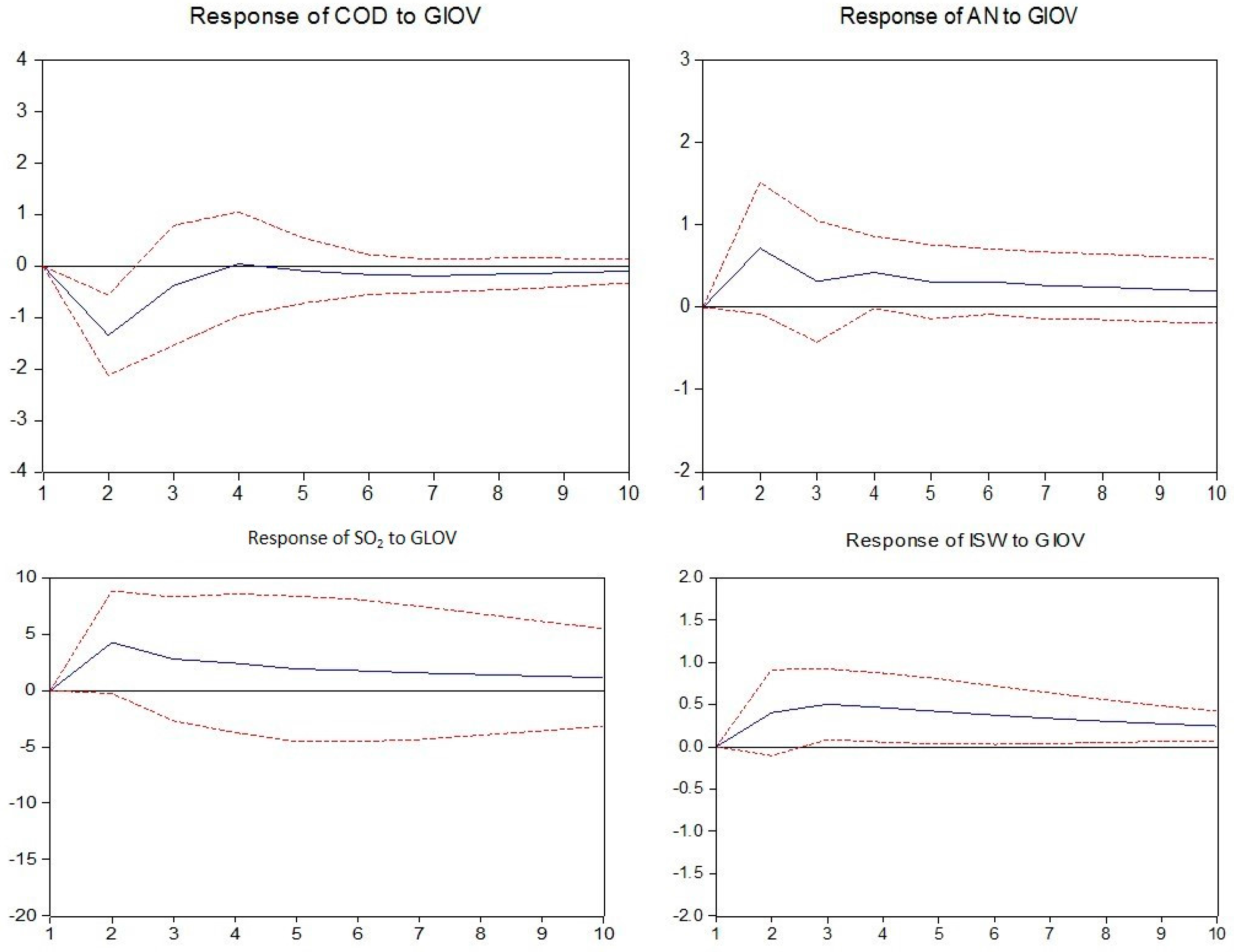
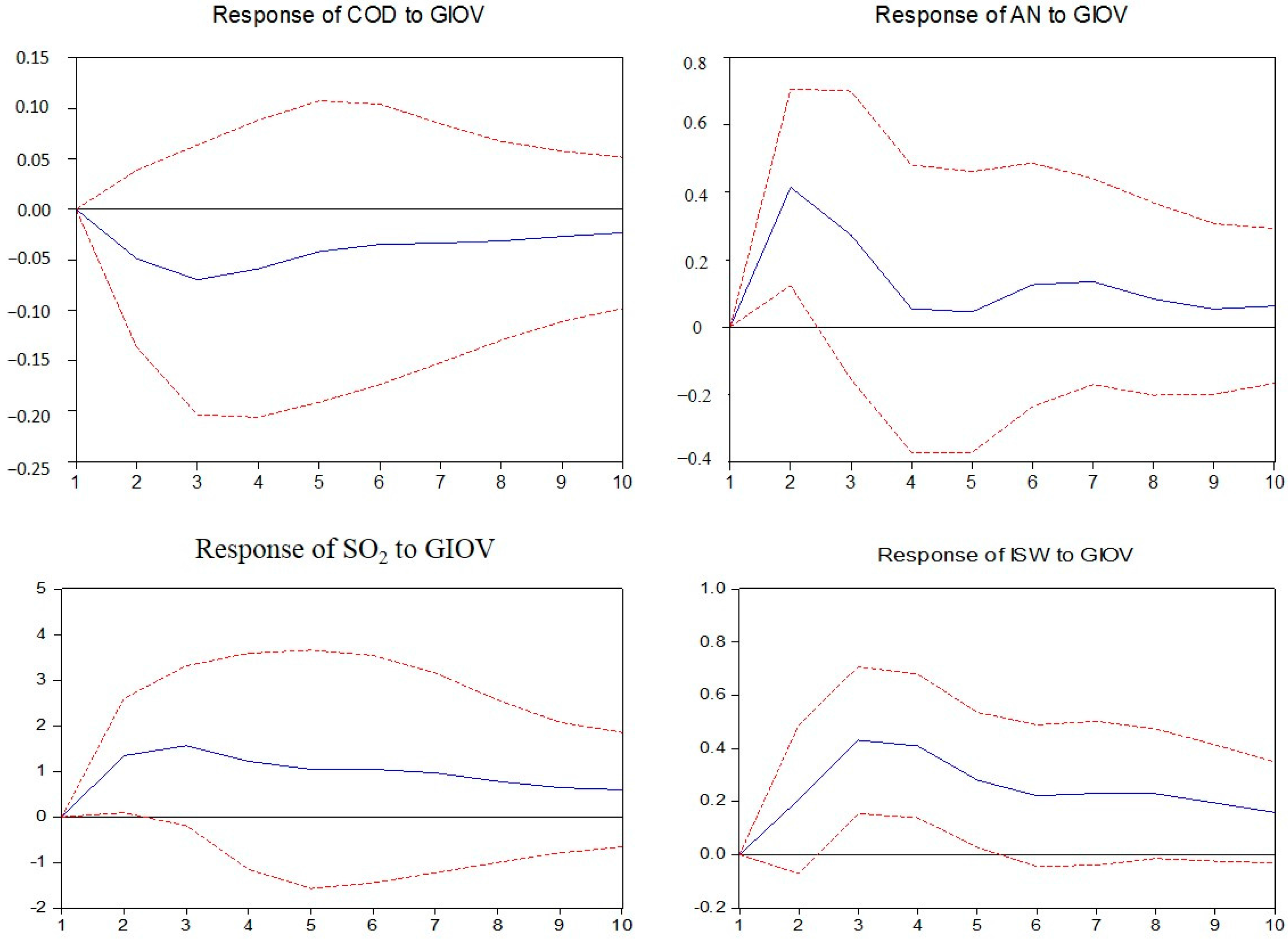
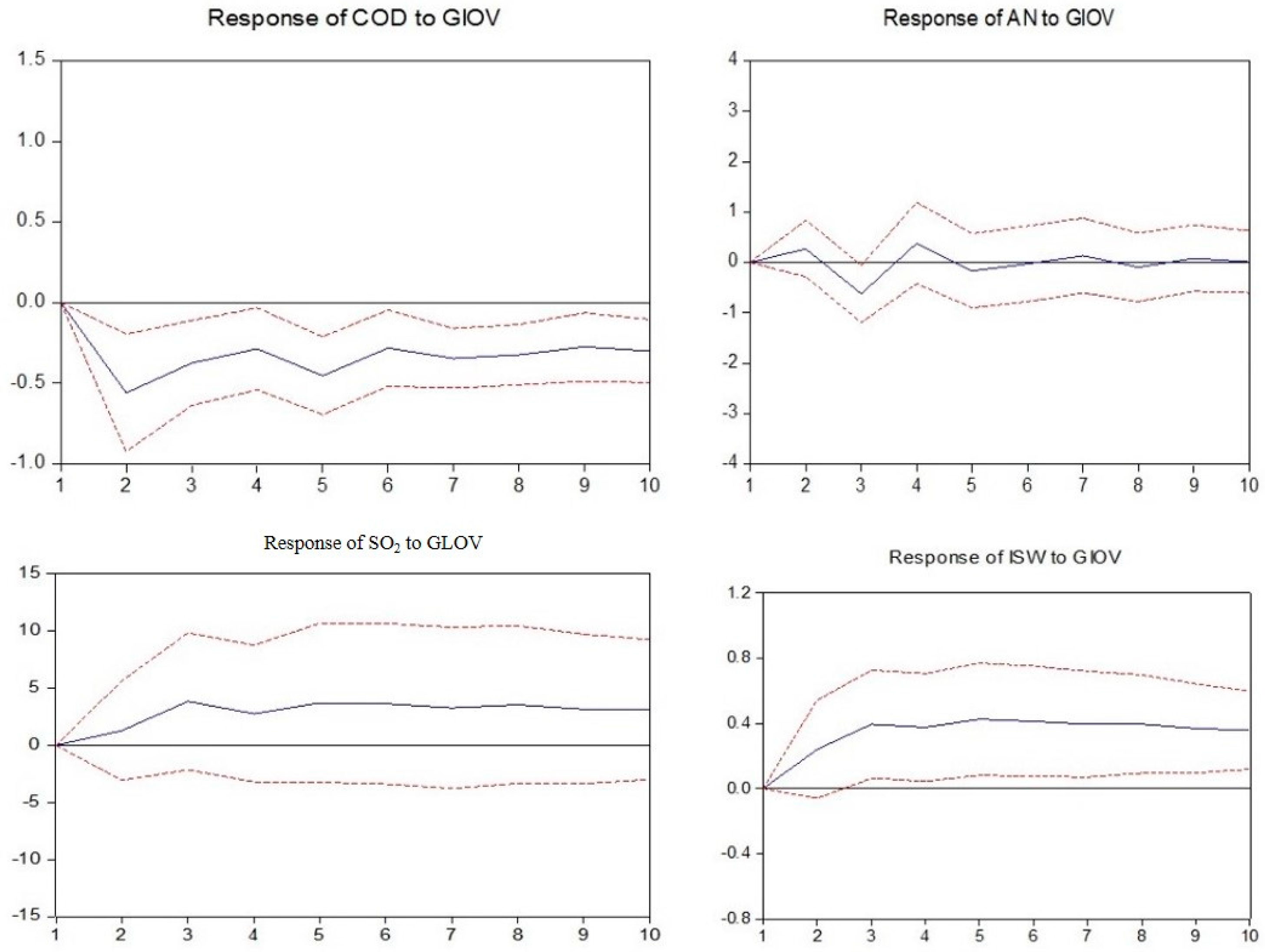
According to the above empirical results, we come to the conclusion that in terms of water pollution, the discharge of COD decreased in coal mining and washing in the short-term but increased in the long-term, whereas it increased in the other industries. The discharge of AN decreased only in petroleum and natural gas extraction and increased in the others. This phenomenon is due to the limiting effect of weak emission standards for mining wastewater and because AN was not used as an indicator for wastewater treatment until 2011 [59]. Although the maximum permissible discharge concentrations of COD and AN are clear in the Integrated Wastewater Discharge Standard [60], to which discharged mining wastewater refers, the following two deficiencies limit the effects of the standard. First, the Integrated Wastewater Discharge Standard is not specific to each industrial sector. The maximum permissible discharge concentrations in this standard are applied to the whole mining industry. The fact that the degree of pollution varies depending on different types of mineral resources has not been considered. Second, the maximum permissible discharge concentrations adopted in 1996 are too high to efficiently control the pollutants. However, COD has been taken as an indicator of sewage treatment in the China Environmental Protection plan, but AN was not used until 2011. Hence, the weak limiting effect of emission standards and the indicators for wastewater treatment that are not specific to each industrial sector caused a decrease in the COD in all types of mining industries (for coal mining and washing, it only decreased in the short-term), but the AN increased in most mining industries except for petroleum and natural gas extraction. The reason for the increase in COD from coal mining and washing in the long-term after decreasing in the short-term is that tactic of increasing production, which is adopted by most coal enterprises to compensate for losses caused by falling coal prices, leads to an increase in the COD discharged per gross industrial output value. The reason the AN only decreased in petroleum and natural gas extraction is that a great deal of industrial wastewater in which the COD is not treated is injected into the oil field. Furthermore, the injection rate is greater than 90%, and this rejected wastewater is not counted as discharged wastewater. Hence, the AN in petroleum and natural gas extraction decreased.

In terms of air pollution, the industrial SO₂ decreased in coal mining and washing, decreased in the short term in petroleum and natural gas extraction, but increased in the long-term and increased in the other three mining industries. The reason for this phenomenon is that the effect of the Integrated Emission Standard of Air Pollutants, to which mining waste gas refers, is not strong due to the same deficiencies as in the Integrated Wastewater Discharge Standard [61]. However, the Discharge Standard for Coal Industry [62] lowered the maximum permissible discharge concentration of industrial SO₂, causing the industrial SO₂ to decrease in coal mining and washing. In addition, the comprehensive utilization of coal gangue decrease the industrial SO₂ to some extent. A large number of coal gangue are produced and are piled up [63]. The coal gangue piles are prone to spontaneous combustion, which is hazardous to environment by discharge the harmful gas including sulfur dioxide. With the increasing awareness of environmental protection and comprehensive utilization of resources in China, the coal gangue is used for power generation and making bricks, etc. This change makes the gangue piles turned into man-made eco-park and decrease the amount of sulfur dioxide discharged [64,65]. The reason the industrial SO₂ decreased in the short-term in petroleum and natural gas extraction is that the industrial SO₂ is mainly produced from natural gas purification plant tail gas and policies were introduced to encourage enterprises to improve the recovery and utilization of industrial SO₂ in the tail gas of these purification plants. Nevertheless, the costs of tail gas treatment and the maximum permissible discharge concentrations for the extraction of petroleum and natural gas are too high. To pursue economic benefits, tail gas treatment equipment is the optimal choice for enterprises. This caused the industrial SO₂ increase in the long-term in petroleum and natural gas extraction.

In terms of solid pollution, the industrial solid waste discharged decreased in petroleum and natural gas extraction, decreased in coal mining and washing in the short-term but increased in the long-term and increased in the three other types of mining industries. This phenomenon occurs because some of the Chinese government’s policies to promote the comprehensive utilization ratio of the industrial solid wastes were only implemented in coal mining and washing and petroleum and natural gas extraction. The comprehensive utilization of 17% of coal gangue is required [66], and a 100% resource utilization ratio of oily sludge is required [67]. Furthermore, the enterprises that sell the coal gangue or oily sludge they produce and those that yield products made of coal gangue or oily sludge can return 50% value-added tax [68]. These policies decreased the industrial solid waste in petroleum and natural gas extraction and in coal mining and washing in the short-term. However, the tactic of increasing production, which is adopted by most coal enterprises to compensate for losses caused by falling coal prices, caused the increase in industrial solid waste in the long-term. In addition to the above three points, the uniformity of the pollution control policies and standards reduce the effect of pollution prevention to some extent because there are diversities in the level of economic development, industrial structure, environmental carrying capacity, etc., among the provinces [69,70,71]. Firstly, although the uniform pollution control policies and standards are stipulated by the central government, the responsibilities of local governments are not clear for environment pollution, and further how such responsibilities are evaluated [72]. In order to economic development, local governments，especially who face difficulty in economic development, are inclined to neglect their responsibilities for protecting local environment, and finally make the effects of uniform pollution control policies and standards unobvious [73,74,75]. Worse still, local governments may reduce the collection of emission fees to protect the profits of local companies [76]. For example, the industrial structure of Shanxi Province is single due to heavily dependent on coal industry. When the coal prices are low, it is a challenge for Shanxi Province to solve environmental problems according to the uniform policies and standards. Secondly, the diversities of environment carrying capacities among provinces can make the different environmental disturbance caused by the same amount of pollution discharged [77,78,79,80]. Therefore, the implementation of the uniform pollution control policies and standards is not rational. It can destruct the environment in ecologically fragile regions due to the low pollutant control polices and standards, which are suitable for regions with high environment carrying capacities. For example, the forest coverage rate and rainfall are low in northwest China, in which most province are environmental fragile. The environment can be construct if these provinces implement the same pollution control policies and standards as other regions.

5. Conclusions

Using a time series from 2001 to 2014, this paper investigated the nexus between industry development and environmental pollution in coal mining and washing, petroleum and natural gas extraction and non-ferrous metal ore, ferrous metal ore and non-metal ore mining and processing in China, considering the dynamic changes within the VAR model. The results are as follows.

The pertinence of standards for the discharge of industrial wastewater and industrial waste gas is not strong and the maximum permissible discharge concentrations in these standards are too high. These two problems limit the effect of the standards in most mineral industries. Hence, to reduce the discharge of pollutants in industrial wastewater and waste gas, niche targeting standards for industrial wastewater and the waste gas should be adopted and the maximum permissible discharge concentrations in the standards should be lowered for different mining industries according to the characteristics of pollutants in each mining industry.

Tax reduction policies to promote the comprehensive utilization of industrial solid waste in coal mining and washing and petroleum and natural gas extraction are effective. However, these policies are not adopted in other mining industries. Hence, to reduce the discharge of industrial solid waste in non-ferrous metal ore, ferrous metal ore and non-metal ore mining and processing, the enterprises that sell the industrial solid waste they produce and those that yield products made of industrial solid waste can return a part of the value-added tax in these three mining industries.

The tactic of increasing production, used by many coal enterprises, led to increases in the COD and industrial solid waste discharged in the long-term in this industry. Hence, to manage the problem of overcapacity of coal enterprises, the production of coal enterprises should be controlled within a reasonable range by the Chinese government. Policies should also be adopted to encourage coal enterprises to extend the industrial chain by developing the coal chemical and coal gasification industries, which can increase the added value of the product to compensate for losses caused by falling prices.

The current uniform pollution control policies and standards have a shortage that they do not consider the diversity among different provinces. The diversity can reduce the effect of pollution prevention. Hence, the different pollution control policies and standards should be stipulated according to the level of economic development, industrial structure, environmental carrying capacity, etc., among provinces. Appropriately raise pollution control polices and standards in environmental fragile regions. Meanwhile, responsibilities of local governments for environment pollution should be determined and the method should be stipulated to evaluate the responsibilities.

References

1. Ministry of Land and Resources of the People’s Republic of China. China Land and Resources Statistical Yearbook; Geological Publishing House: Beijing, China, 2015.
2. National Bureau of Statistics. China Industry Economy Statistical Yearbook; China Statistics Press: Beijing, China, 2002.
3. National Bureau of Statistics. China Industry Economy Statistical Yearbook; China Statistics Press: Beijing, China, 2003.
4. National Bureau of Statistics. China Industry Economy Statistical Yearbook; China Statistics Press: Beijing, China, 2004.
5. National Bureau of Statistics. China Industry Economy Statistical Yearbook; China Statistics Press: Beijing, China, 2005.
6. National Bureau of Statistics. China Industry Economy Statistical Yearbook; China Statistics Press: Beijing, China, 2006.
7. National Bureau of Statistics. China Industry Economy Statistical Yearbook; China Statistics Press: Beijing, China, 2007.
8. National Bureau of Statistics. China Industry Economy Statistical Yearbook; China Statistics Press: Beijing, China, 2008.
9. National Bureau of Statistics. China Industry Economy Statistical Yearbook; China Statistics Press: Beijing, China, 2009.
10. National Bureau of Statistics. China Industry Economy Statistical Yearbook; China Statistics Press: Beijing, China, 2010.
11. National Bureau of Statistics. China Industry Economy Statistical Yearbook; China Statistics Press: Beijing, China, 2011.
12. National Bureau of Statistics. China Industry Economy Statistical Yearbook; China Statistics Press: Beijing, China, 2012.
13. National Bureau of Statistics. China Industry Statistical Yearbook; China Statistics Press: Beijing, China, 2013.
14. National Bureau of Statistics. China Industry Statistical Yearbook; China Statistics Press: Beijing, China, 2014.
15. National Bureau of Statistics. China Industry Statistical Yearbook; China Statistics Press: Beijing, China, 2015.
16. National Bureau of Statistics. China Statistical Yearbook; China Statistics Press: Beijing, China, 2002.
17. National Bureau of Statistics. China Statistical Yearbook; China Statistics Press: Beijing, China, 2003.
18. National Bureau of Statistics. China Statistical Yearbook; China Statistics Press: Beijing, China, 2004.
19. National Bureau of Statistics. China Statistical Yearbook; China Statistics Press: Beijing, China, 2005.
20. National Bureau of Statistics. China Statistical Yearbook; China Statistics Press: Beijing, China, 2006.
21. National Bureau of Statistics. China Statistical Yearbook; China Statistics Press: Beijing, China, 2007.
22. National Bureau of Statistics. China Statistical Yearbook; China Statistics Press: Beijing, China, 2008.
23. National Bureau of Statistics. China Statistical Yearbook; China Statistics Press: Beijing, China, 2009.
24. National Bureau of Statistics. China Statistical Yearbook; China Statistics Press: Beijing, China, 2010.
25. National Bureau of Statistics. China Statistical Yearbook; China Statistics Press: Beijing, China, 2011.
26. National Bureau of Statistics. China Statistical Yearbook; China Statistics Press: Beijing, China, 2012.
27. National Bureau of Statistics. China Statistical Yearbook; China Statistics Press: Beijing, China, 2013.
28. National Bureau of Statistics. China Statistical Yearbook; China Statistics Press: Beijing, China, 2014.
29. National Bureau of Statistics. China Statistical Yearbook; China Statistics Press: Beijing, China, 2015.
30. The Central People’s Government of the People’s Republic of China. National Resources city Sustainable development Planning (2013–2020). Available online: http://www.gov.cn/zwgk/2013-12/03/content_2540070.htm (accessed on 12 December 2013).
31. National Bureau of Statistics. China Statistical Yearbook on Environment; China Statistics Press: Beijing, China, 2002.
32. National Bureau of Statistics. China Statistical Yearbook on Environment; China Statistics Press: Beijing, China, 2003.
33. National Bureau of Statistics. China Statistical Yearbook on Environment; China Statistics Press: Beijing, China, 2004.
34. National Bureau of Statistics. China Statistical Yearbook on Environment; China Statistics Press: Beijing, China, 2005.
35. National Bureau of Statistics. China Statistical Yearbook on Environment; China Statistics Press: Beijing, China, 2006.
36. National Bureau of Statistics. China Statistical Yearbook on Environment; China Statistics Press: Beijing, China, 2007.
37. National Bureau of Statistics. China Statistical Yearbook on Environment; China Statistics Press: Beijing, China, 2008.
38. National Bureau of Statistics. China Statistical Yearbook on Environment; China Statistics Press: Beijing, China, 2009.
39. National Bureau of Statistics. China Statistical Yearbook on Environment; China Statistics Press: Beijing, China, 2010.
40. National Bureau of Statistics. China Statistical Yearbook on Environment; China Statistics Press: Beijing, China, 2011.
41. National Bureau of Statistics. China Statistical Yearbook on Environment; China Statistics Press: Beijing, China, 2012.
42. National Bureau of Statistics. China Statistical Yearbook on Environment; China Statistics Press: Beijing, China, 2013.
43. National Bureau of Statistics. China Statistical Yearbook on Environment; China Statistics Press: Beijing, China, 2014.
44. National Bureau of Statistics. China Statistical Yearbook on Environment; China Statistics Press: Beijing, China, 2015.
45. Bloch, H.; Rafiq, S.; Salim, R. Coal consumption, CO2 emission and economic growth in China: Empirical evidence and policy responses. Energy Econ. 2012, 34, 518–528. [Google Scholar] [CrossRef]
46. Saboori, B.; Sulaiman, J. Environmental degradation, economic growth and energy consumption: Evidence of the environmental kuznets curve in Malaysia. Energy Policy 2013, 60, 892–905. [Google Scholar] [CrossRef]
47. Tiwari, A.K.; Shahbaz, M.; Adnan Hye, Q.M. The environmental kuznets curve and the role of coal consumption in India: Cointegration and causality analysis in an open economy. Renew. Sustain. Energy Rev. 2013, 18, 519–527. [Google Scholar] [CrossRef] [Green Version]
48. Ahmad, A.; Zhao, Y.; Shahbaz, M.; Bano, S.; Zhang, Z.; Wang, S.; Liu, Y. Carbon emissions, energy consumption and economic growth: An aggregate and disaggregate analysis of the Indian economy. Energy Policy 2016, 96, 131–143. [Google Scholar] [CrossRef]
49. Govindaraju, V.G.R.C.; Tang, C.F. The dynamic links between CO2 emissions, economic growth and coal consumption in China and India. Appl. Energy 2013, 104, 310–318. [Google Scholar] [CrossRef]
50. Guo, W.; Kar, A. Energy consumption, carbon emissions and economic growth in Saudiarabia: An aggregate and disaggregate analysis. Energy Policy 2013, 62, 1525–1532. [Google Scholar]
51. Yu, S.; Wei, Y.M. Prediction of China’s coal production-environmental pollution based on a hybrid genetic algorithm-system dynamics model. Energy Policy 2012, 42, 521–529. [Google Scholar] [CrossRef]
52. Xu, B.; Lin, B. Carbon dioxide emissions reduction in China’s transport sector: A dynamic var (vector autoregression) approach. Energy 2015, 83, 486–495. [Google Scholar] [CrossRef]
53. Nyberg, H.; Saikkonen, P. Forecasting with a noncausal var model. Comput. Stat. Data Anal. 2014, 76, 536–555. [Google Scholar] [CrossRef]
54. Abbasi, F.; Riaz, K. CO2 emissions and financial development in an emerging economy: An augmented var approach. Energy Policy 2016, 90, 102–114. [Google Scholar] [CrossRef]
55. Calcagnini, G.; Giombini, G.; Travaglini, G. Modelling energy intensity, pollution per capita and productivity in Italy: A structural var approach. Renew. Sustain. Energy Rev. 2016, 59, 1482–1492. [Google Scholar] [CrossRef]
56. Cologni, A.; Manera, M. Oil prices, inflation and interest rates in a structural cointegrated var model for the G-7 countries. Energy Econ. 2008, 30, 856–888. [Google Scholar] [CrossRef]
57. Magkonis, G.; Tsopanakis, A. Exploring the effects of financial and fiscal vulnerabilities on G7 economies: Evidence from SVAR analysis. J. Int. Financ. Markets Inst. Money 2014, 32, 343–367. [Google Scholar] [CrossRef]
58. Engle, R.E.; Granger, C.W.J.; Engle, R.E.; Granger, C.W.J. Cointegration and equilibrium correction representation, estimation and testing. Econometrica 1987, 55, 251–276. [Google Scholar] [CrossRef]
59. The Central People’s Government of the People’s Republic of China. National “12th Five-Year Plan” for Environmental Protection. Available online: http://www.gov.cn/zwgk/2011-12/20/content_2024895.htm (accessed on 15 December 2011).
60. Ministry of Environmental Protection of the People’s Republic of China. Integrated Wastewater Discharge Standard (GB 8978-1996). Available online: http://chinawaterrisk.org/research-reports/integrated-wastewater-discharge-standard-gb-8978-1996/ (accessed on 6 September 2016).
61. Ministry of Environmental Protection of the People’s Republic of China. Integrated Emission Standard of Air Pollutants (GB 162797-1996). Available online: http://english.mep.gov.cn/standards_reports/standards/Air_Environment/Emission_standard1/200710/t20071024_111824.htm (accessed on 6 September 2016).
62. Ministry of Environmental Protection of the People’s Republic of China. Emission Standard for Pollutants from Coal Industry (GB 20426-2006). Available online: http://english.mep.gov.cn/standards_reports/standards/Air_Environment/Emission_standard1/200710/t20071024_111830.htm (accessed on 6 September 2016).
63. Querol, X.; Izquierdo, M.; Monfort, E.; Alvarez, E.; Font, O.; Moreno, T.; Alastuey, A.; Zhuang, X.; Lu, W.; Wang, Y. Environmental characterization of burnt coal gangue banks at Yangquan, Shanxi province, China. Int. J. Coal Geology 2008, 75, 93–104. [Google Scholar] [CrossRef]
64. Haibin, L.; Zhenling, L. Recycling utilization patterns of coal mining waste in China. Resour. Conserv. Recycl. 2010, 54, 1331–1340. [Google Scholar] [CrossRef]
65. Zhou, C.; Liu, G.; Wu, S.; Lam, P.K.S. The environmental characteristics of usage of coal gangue in bricking-making: A case study at Huainan, China. Chemosphere 2014, 95, 274–280. [Google Scholar] [CrossRef] [PubMed]
66. Ministry of Land and Resources of the People’s Republic of China. Announcement of “Three Rate” Index Requirements of Coal Resources Rational Development and Utilization. Available online: http://www.mlr.gov.cn/zwgk/zytz/201209/t20120925_1143729.htm (accessed on 20 September 2012).
67. Ministry of Environmental Protection of the People’s Republic of China. Policy of Pollutant Prevention and Control Technology in Oil and Gas Exploitation Industry. Available online: http://kjs.mep.gov.cn/hjbhbz/bzwb/wrfzjszc/201203/t20120319_224789.shtml (accessed on 7 March 2012).
68. State Administration of Taxation. Announcement of the Policy of Adjusting the Value Added Tax of Products and Services to the Comprehensive Utilization of Resources. Available online: http://www.chinatax.gov.cn/2013/n2226/n2271/n2272/c121831/content.html (accessed on 9 September 2016).
69. Zhang, C.; Zhou, K.; Yang, S.; Shao, Z. Exploring the transformation and upgrading of China’s economy using electricity consumption data: A var-vec based model. Physica A 2017, 473, 144–155. [Google Scholar] [CrossRef]
70. Gao, J.; Yuan, Z.; Liu, X.; Xia, X.; Huang, X.; Dong, Z. Improving air pollution control policy in China—A perspective based on cost-benefit analysis. Sci. Total Environ. 2016, 543, 307–314. [Google Scholar] [CrossRef] [PubMed]
71. Liu, G.; Yang, Z.; Chen, B.; Zhang, Y.; Su, M.; Ulgiati, S. Prevention and control policy analysis for energy-related regional pollution management in China. Appl. Energy 2016, 166, 292–300. [Google Scholar] [CrossRef]
72. Feng, L.; Liao, W. Legislation, plans, and policies for prevention and control of air pollution in China: Achievements, challenges, and improvements. J. Clean. Prod. 2016, 112, 1549–1558. [Google Scholar] [CrossRef]
73. Zhang, Q.; He, K.; Huo, H. Policy: Cleaning China’s air. Nature 2012, 484, 161–162. [Google Scholar] [PubMed]
74. Zheng, D.; Shi, M. Multiple environmental policies and pollution haven hypothesis: Evidence from China’s polluting industries. J. Clean. Prod. 2017, 141, 295–304. [Google Scholar] [CrossRef]
75. Zhou, Y.; Zhu, S.; He, C. How do environmental regulations affect industrial dynamics? Evidence from China’s pollution-intensive industries. Habitat Int. 2017, 60, 10–18. [Google Scholar] [CrossRef]
76. Zhang, X.; Ortolano, L.; Lü, Z. Agency empowerment through the administrative litigation law: Court enforcement of pollution levies in Hubei province. China Q. 2010, 202, 307–326. [Google Scholar] [CrossRef]
77. Wang, R.; Cheng, J.; Zhu, Y.; Xiong, W. Research on diversity of mineral resources carrying capacity in Chinese mining cities. Resour. Policy 2016, 47, 108–114. [Google Scholar] [CrossRef]
78. Zhang, Q.; Miao, L.; Wang, X.; Liu, D.; Zhu, L.; Zhou, B.; Sun, J.; Liu, J. The capacity of greening roof to reduce stormwater runoff and pollution. Landsc. Urban Plann. 2015, 144, 142–150. [Google Scholar] [CrossRef]
79. Li, N.; Yang, H.; Wang, L.; Huang, X.; Zeng, C.; Wu, H.; Ma, X.; Song, X.; Wei, Y. Optimization of industry structure based on water environmental carrying capacity under uncertainty of the huai river basin within Shandong province, China. J. Clean. Prod. 2016, 112, 4594–4604. [Google Scholar] [CrossRef]
80. Kang, P.; Xu, L. Water environmental carrying capacity assessment of an industrial park. Procedia Environ. Sci. 2012, 13, 879–890. [Google Scholar] [CrossRef]
Figure 1. Industrial sales value of mining industrial over 2001–2014.
Ijerph 14 00254 g001
Figure 2. Three wastes emissions over 2001–2014.
Ijerph 14 00254 g002
Figure 3. VAR roots of characteristic polynomial of mining and washing of coal. Note: blue dots indicate characteristic roots.
Ijerph 14 00254 g003
Figure 4. VAR roots of characteristic polynomial of extraction of petroleum and natural gas. Note: blue dots indicate characteristic roots.
Ijerph 14 00254 g004
Figure 5. VAR roots of characteristic polynomial of mining and processing of non-ferrous metal ores. Note: blue dots indicate characteristic roots.
Ijerph 14 00254 g005
Figure 6. VAR roots of characteristic polynomial of mining and processing of ferrous metal ores. Note: blue dots indicate characteristic roots.
Ijerph 14 00254 g006
Figure 7. VAR roots of characteristic polynomial of mining and processing of nonmetal ores. Note: blue dots indicate characteristic roots.
Ijerph 14 00254 g007
Figure 8. Responses of pollutants charged to industrial output value of mining and washing of coal. The solid lines indicate the mean responses to a one standard deviation shock, while the dotted lines represent ± 2 standard deviations of the responses.
Ijerph 14 00254 g008
Figure 9. Responses of pollutants charged to industrial output value of extraction of petroleum and natural gas. The solid lines indicate the mean responses to a one standard deviation shock, while the dotted lines represent ± 2 standard deviations of the responses.
Ijerph 14 00254 g009
Figure 10. Responses of pollutants charged to industrial output value of mining and processing of non-ferrous metal ores. The solid lines indicate the mean responses to a one standard deviation shock, while the dotted lines represent ± 2 standard deviations of the responses.
Ijerph 14 00254 g010
Figure 11. Responses of pollutants charged to industrial output value of mining and processing of ferrous metal ores. The solid lines indicate the mean responses to a one standard deviation shock, while the dotted lines represent ± 2 standard deviations of the responses.
Ijerph 14 00254 g011
Figure 12. Responses of pollutants charged to industrial output value of mining and processing of nonmetal ores. The solid lines indicate the mean responses to a one standard deviation shock, while the dotted lines represent ± 2 standard deviations of the responses.
Ijerph 14 00254 g012