Using Individual GPS Trajectories to Explore Foodscape Exposure: A Case Study in Beijing Metropolitan Area


Abstract
:1. Introduction
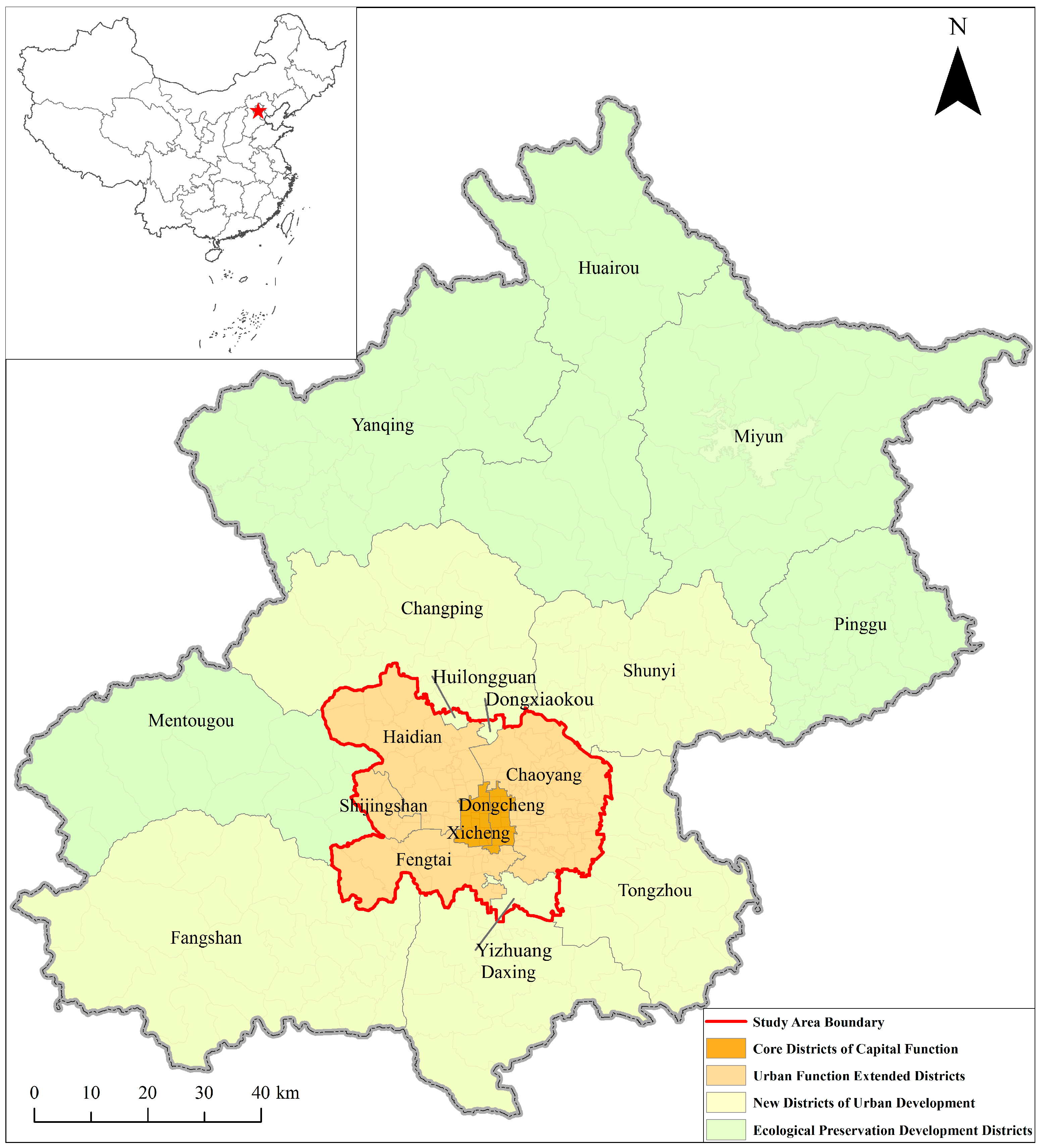
2. Study Dataset
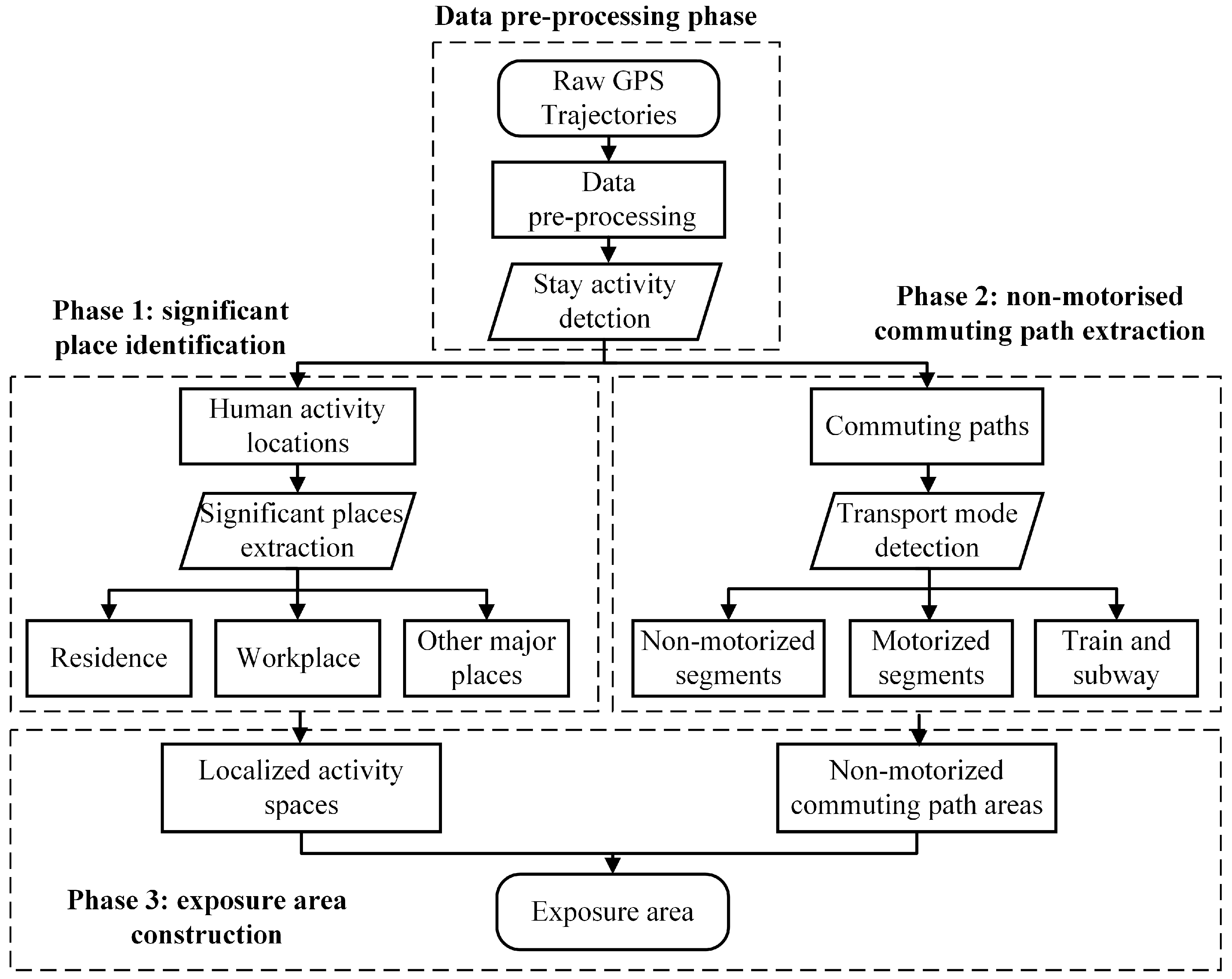
3. Methodology
3.1. Identification of Significant Places
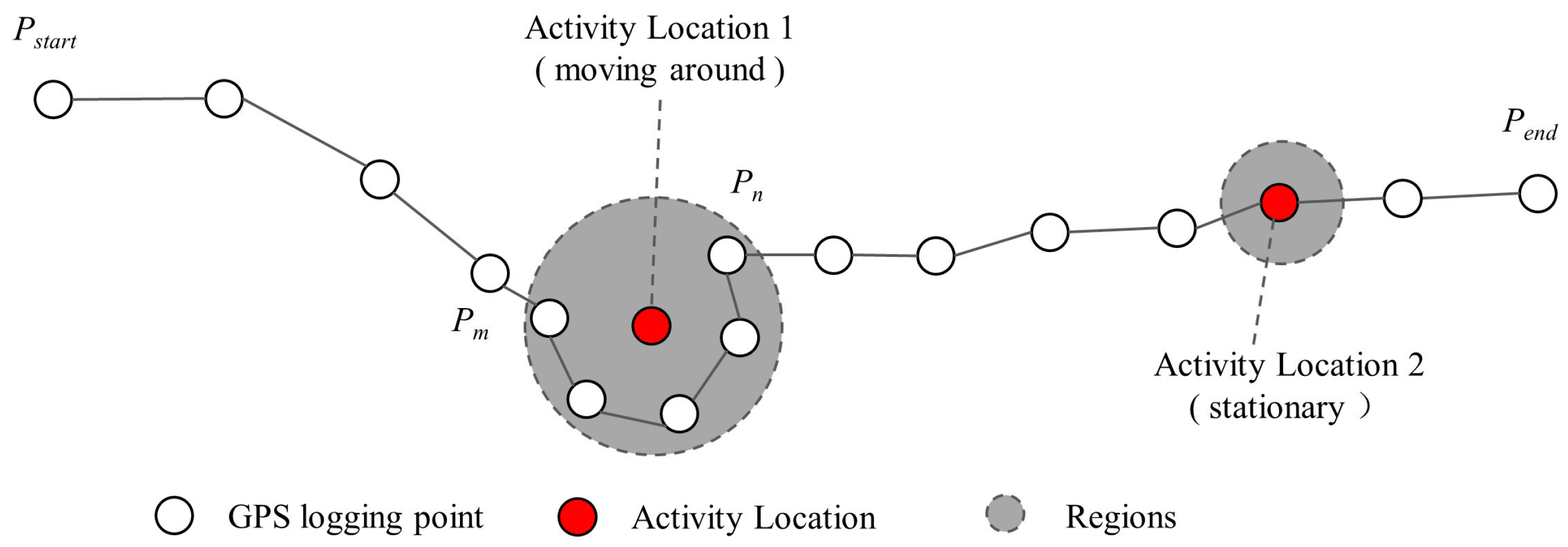
3.1.1. Step 1: Extraction of Activity Locations
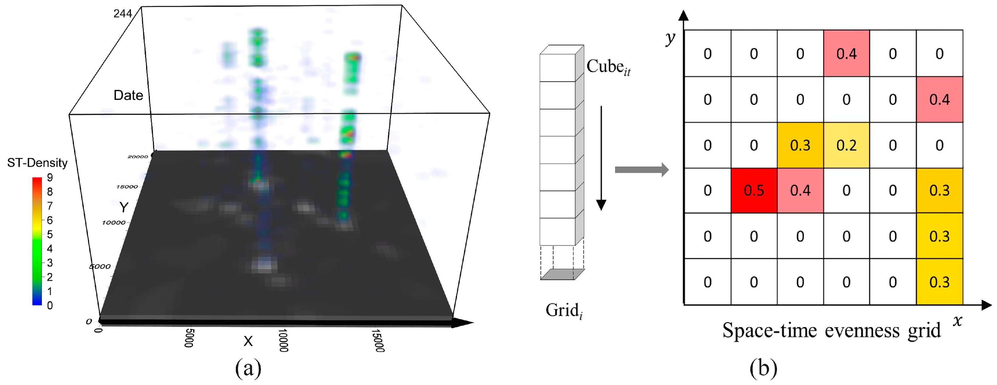
3.1.2. Step 2: Detection of Significant Place Candidates
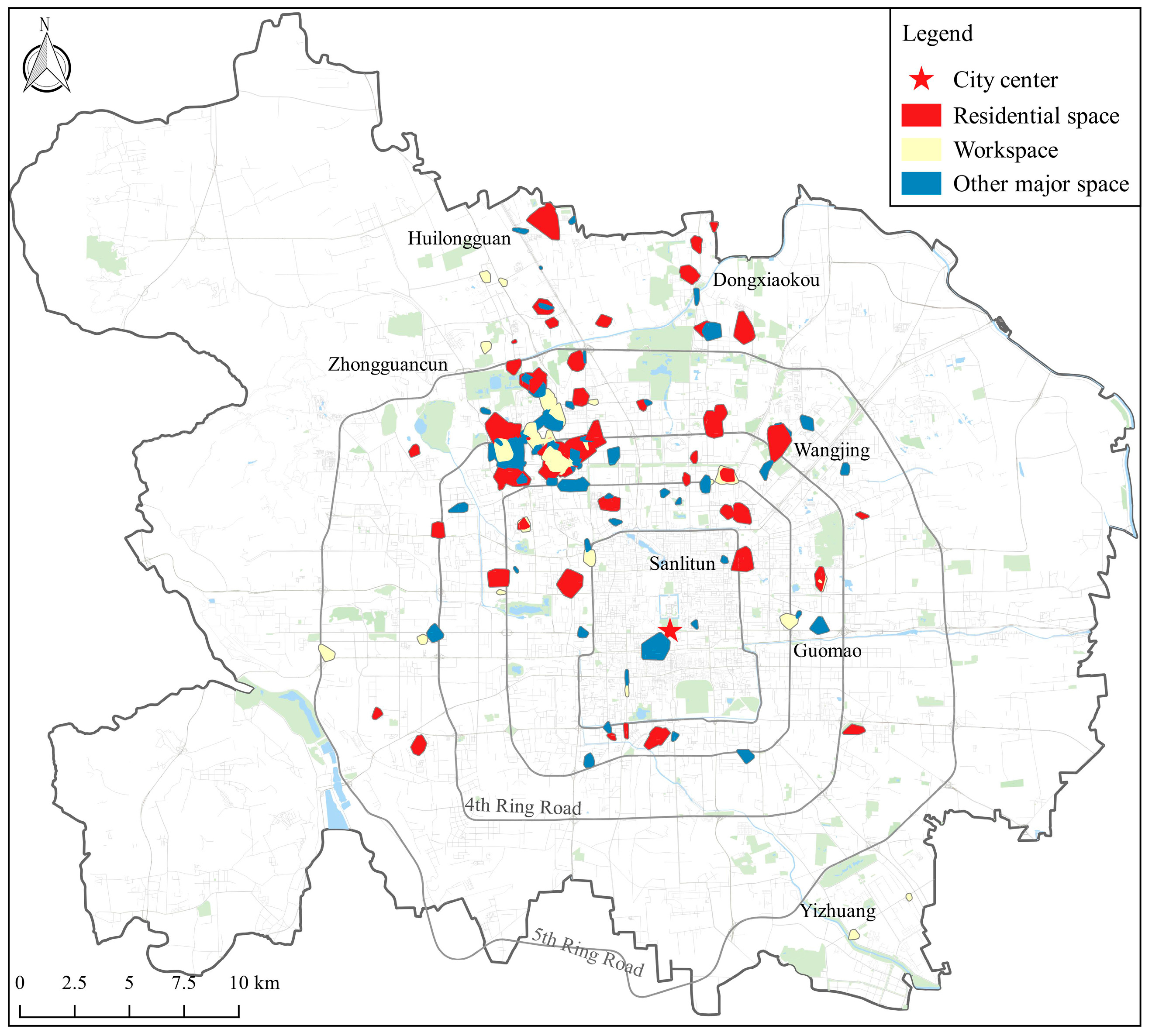
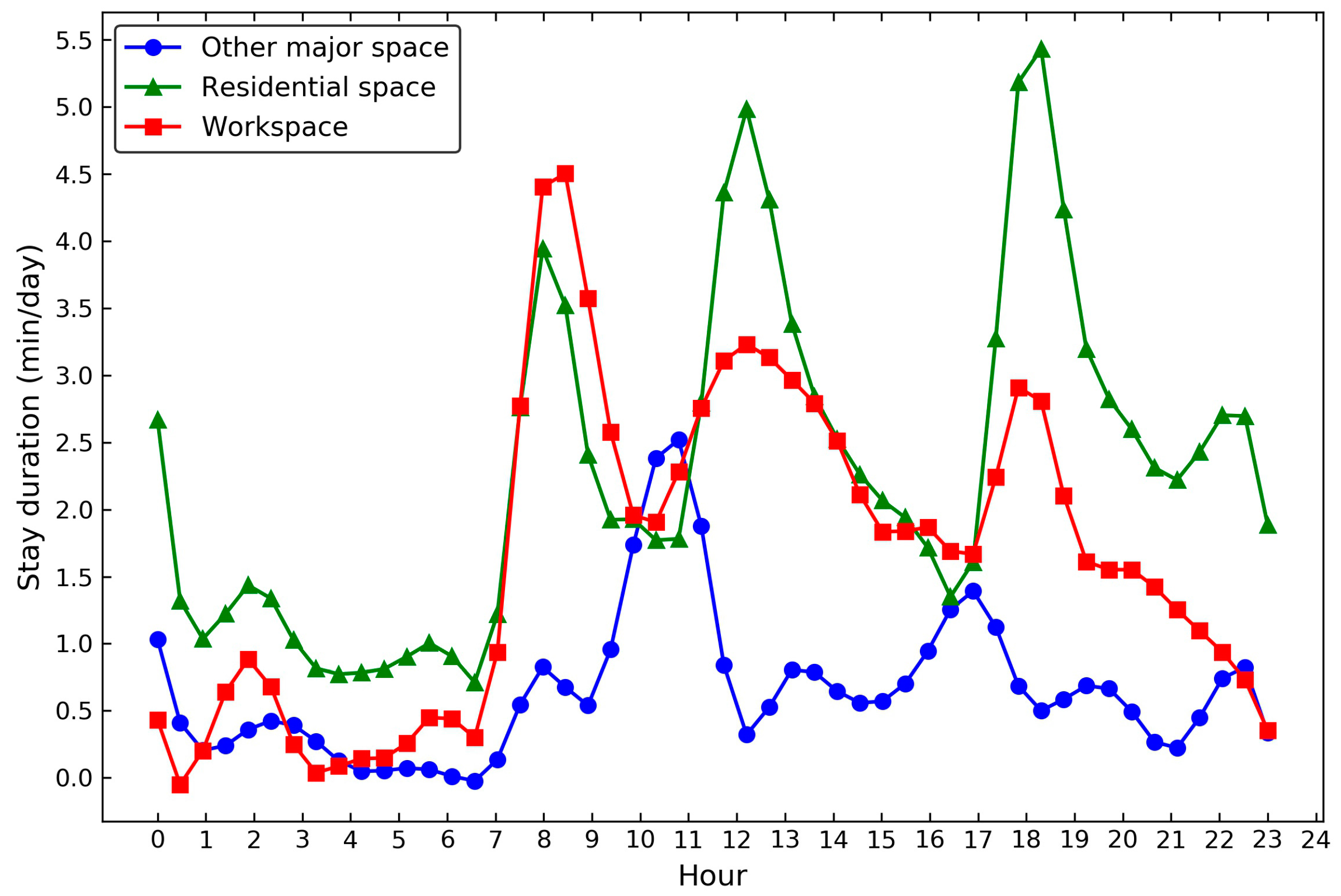
3.1.3. Step 3: Labeling of Significant Places
3.2. Extraction of Non-Motorized Routes
3.3. Construction of Exposure Area
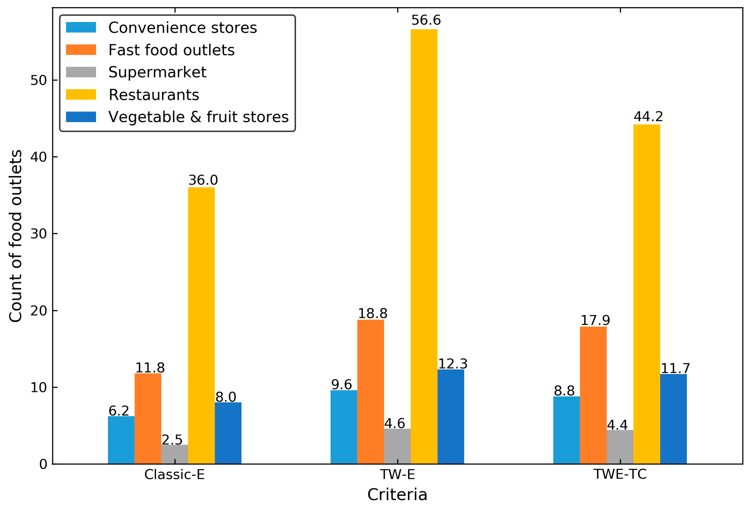
3.4. Food Environmental Exposure Evaluation
4. Results
4.1. Description of the Study Sample
4.2. Analysis of Foodscape Exposure in Multiple Context
4.3. Analysis of Overall Foodscape Exposure
5. Discussion
5.1. Main Findings
5.2. Strengths and Limitations
6. Conclusions
Supplementary Materials
Acknowledgments
Author Contributions
Conflicts of Interest
References
- Kwan, M.-P. Geographies of health. Ann. Assoc. Am. Geogr. 2012, 102, 891–892. [Google Scholar] [CrossRef]
- Berke, E.M.; Koepsell, T.D.; Moudon, A.V.; Hoskins, R.E.; Larson, E.B. Association of the built environment with physical activity and obesity in older persons. Am. J. Public Health 2007, 97, 486–492. [Google Scholar] [CrossRef] [PubMed]
- Dubowitz, T.; Zenk, S.N.; Ghosh-Dastidar, B.; Cohen, D.A.; Beckman, R.; Hunter, G.; Steiner, E.D.; Collins, R.L. Healthy food access for urban food desert residents: Examination of the food environment, food purchasing practices, diet and BMI. Public Health Nutr. 2015, 18, 2220–2230. [Google Scholar] [CrossRef] [PubMed]
- Inagami, S.; Cohen, D.A.; Brown, A.F.; Asch, S.M. Body mass index, neighborhood fast food and restaurant concentration, and car ownership. J. Urban Health 2009, 86, 683–695. [Google Scholar] [CrossRef] [PubMed]
- Pearce, J.; Hiscock, R.; Blakely, T.; Witten, K. The contextual effects of neighbourhood access to supermarkets and convenience stores on individual fruit and vegetable consumption. J. Epidemiol. Community Health 2008, 62, 198–201. [Google Scholar] [CrossRef] [PubMed]
- Laska, M.N.; Hearst, M.O.; Forsyth, A.; Pasch, K.E.; Lytle, L. Neighbourhood food environments: Are they associated with adolescent dietary intake, food purchases and weight status? Public Health Nutr. 2010, 13, 1757–1763. [Google Scholar] [CrossRef] [PubMed]
- Kwan, M.P. From place-based to people-based exposure measures. Soc. Sci. Med. 2009, 69, 1311–1313. [Google Scholar] [CrossRef] [PubMed]
- Perchoux, C.; Chaix, B.; Cummins, S.; Kestens, Y. Conceptualization and measurement of environmental exposure in epidemiology: Accounting for activity space related to daily mobility. Health Place 2013, 21, 86–93. [Google Scholar] [CrossRef] [PubMed]
- Basta, L.A.; Richmond, T.S.; Wiebe, D.J. Neighborhoods, daily activities, and measuring health risks experienced in urban environments. Soc. Sci. Med. 2010, 71, 1943–1950. [Google Scholar] [CrossRef] [PubMed]
- Troped, P.J.; Wilson, J.S.; Matthews, C.E.; Cromley, E.K.; Melly, S.J. The built environment and location-based physical activity. Am. J. Prev. Med. 2010, 38, 429–438. [Google Scholar] [CrossRef] [PubMed]
- Shareck, M.; Kestens, Y.; Frohlich, K.L. Moving beyond the residential neighborhood to explore social inequalities in exposure to area-level disadvantage: Results from the interdisciplinary study on inequalities in smoking. Soc. Sci. Med. 2014, 108, 106–114. [Google Scholar] [CrossRef] [PubMed]
- Richardson, D.B.; Volkow, N.D.; Kwan, M.P.; Kaplan, R.M.; Goodchild, M.F.; Croyle, R.T. Medicine. Spatial turn in health research. Science 2013, 339, 1390–1392. [Google Scholar] [CrossRef] [PubMed]
- Boruff, B.J.; Nathan, A.; Nijënstein, S. Using GPS technology to (re)-examine operational definitions of ‘neighbourhood’ in place-based health research. Int. J. Health Geogr. 2012, 11, 22. [Google Scholar] [CrossRef] [PubMed] [Green Version]
- Kestens, Y.; Lebel, A.; Chaix, B.; Clary, C.; Daniel, M.; Pampalon, R.; Theriault, M.; Subramanian, S.V.P. Association between activity space exposure to food establishments and individual risk of overweight. PLoS ONE 2012, 7, e41418. [Google Scholar]
- Shearer, C.; Rainham, D.; Blanchard, C.; Dummer, T.; Lyons, R.; Kirk, S. Measuring food availability and accessibility among adolescents: Moving beyond the neighbourhood boundary. Soc. Sci. Med. 2015, 133, 322–330. [Google Scholar] [CrossRef] [PubMed]
- Christian, W.J. Using geospatial technologies to explore activity-based retail food environments. Spat. Spatio-Temporal Epidemiol. 2012, 3, 287–295. [Google Scholar] [CrossRef] [PubMed]
- Cetateanu, A.; Jones, A. How can GPS technology help us better understand exposure to the food environment? A systematic review. SSM Popul. Health 2016, 2, 196–205. [Google Scholar] [CrossRef] [PubMed] [Green Version]
- Gustafson, A.; Christian, J.W.; Lewis, S.; Moore, K.; Jilcott, S. Food venue choice, consumer food environment, but not food venue availability within daily travel patterns are associated with dietary intake among adults, Lexington Kentucky 2011. Nutr. J. 2013, 12, 17. [Google Scholar] [CrossRef] [PubMed]
- Rainham, D.; McDowell, I.; Krewski, D.; Sawada, M. Conceptualizing the healthscape: Contributions of time geography, location technologies and spatial ecology to place and health research. Soc. Sci. Med. 2010, 70, 668–676. [Google Scholar] [CrossRef] [PubMed]
- Zenk, S.N.; Schulz, A.J.; Matthews, S.A.; Odoms-Young, A.; Wilbur, J.; Wegrzyn, L.; Gibbs, K.; Braunschweig, C.; Stokes, C. Activity space environment and dietary and physical activity behaviors: A pilot study. Health Place 2011, 17, 1150–1161. [Google Scholar] [CrossRef] [PubMed]
- Matthews, S.A.; Yang, T.C. Spatial polygamy and contextual exposures (spaces): Promoting activity space approaches in research on place and health. Am. Behav. Sci. 2013, 57, 1057–1081. [Google Scholar] [CrossRef] [PubMed]
- Kwan, M.-P. Beyond space (as we knew it): Toward temporally integrated geographies of segregation, health, and accessibility. Ann. Assoc. Am. Geogr. 2013, 103, 1078–1086. [Google Scholar] [CrossRef]
- Axhausen, K.W.; Zimmermann, A.; Schönfelder, S.; Rindsfüser, G.; Haupt, T. Observing the rhythms of daily life: A six-week travel diary. Transportation 2002, 29, 95–124. [Google Scholar] [CrossRef]
- Chaix, B.; Kestens, Y.; Perchoux, C.; Karusisi, N.; Merlo, J.; Labadi, K. An interactive mapping tool to assess individual mobility patterns in neighborhood studies. Am. J. Prev. Med. 2012, 43, 440–450. [Google Scholar] [CrossRef] [PubMed]
- Holliday, K.M.; Howard, A.G.; Emch, M.; Rodriguez, D.A.; Evenson, K.R. Are buffers around home representative of physical activity spaces among adults? Health Place 2017, 45, 181–188. [Google Scholar] [CrossRef] [PubMed]
- Chaix, B.; Meline, J.; Duncan, S.; Merrien, C.; Karusisi, N.; Perchoux, C.; Lewin, A.; Labadi, K.; Kestens, Y. GPS tracking in neighborhood and health studies: A step forward for environmental exposure assessment, a step backward for causal inference? Health Place 2013, 21, 46–51. [Google Scholar] [CrossRef] [PubMed]
- Kwan, M.-P. The uncertain geographic context problem. Ann. Assoc. Am. Geogr. 2012, 102, 958–968. [Google Scholar] [CrossRef]
- Matthews, S.A. Uncertain geographic context problem. In International Encyclopedia of Geography: People, the Earth, Environment and Technology; John Wiley & Sons, Ltd.: Hoboken, NJ, USA, 2016. [Google Scholar]
- Chen, X.; Kwan, M.-P. Contextual uncertainties, human mobility, and perceived food environment: The uncertain geographic context problem in food access research. Am. J. Public Health 2015, 105, 1734–1737. [Google Scholar] [CrossRef] [PubMed]
- Cetateanu, A.; Luca, B.-A.; Popescu, A.A.; Page, A.; Cooper, A.; Jones, A. A novel methodology for identifying environmental exposures using GPS data. Int. J. Geogr. Inf. Sci. 2016, 30, 1944–1960. [Google Scholar] [CrossRef] [Green Version]
- Lipperman-Kreda, S.; Morrison, C.; Grube, J.W.; Gaidus, A. Youth activity spaces and daily exposure to tobacco outlets. Health Place 2015, 34, 30–33. [Google Scholar] [CrossRef] [PubMed]
- Lyseen, A.K.; Hansen, H.S.; Harder, H.; Jensen, A.S.; Mikkelsen, B.E. Defining neighbourhoods as a measure of exposure to the food environment. Int. J. Environ. Res. Public Health 2015, 12, 8504–8525. [Google Scholar] [CrossRef] [PubMed]
- Ester, M.; Kriegel, H.-P.; Sander, J.; Xu, X. Density-based spatial clustering of applications with noise. In Proceedings of the International Conference on Knowledge Discovery and Data Mining, Portland, OR, USA, 2–4 August 1996. [Google Scholar]
- Brunsdon, C.; Corcoran, J.; Higgs, G. Visualising space and time in crime patterns: A comparison of methods. Comput. Environ. Urban Syst. 2007, 31, 52–75. [Google Scholar] [CrossRef]
- Stochastic Gradient Descent Classifier. Available online: http://scikit-learn.org/stable/modules/generated/sklearn.linear_model.SGDClassifier.html (accessed on 9 August 2017).
- Zheng, Y.; Xie, X.; Ma, W.Y. Geolife: A collaborative social networking service among user, location and trajectory. IEEE Data Eng. Bull. 2010, 33, 32–39. [Google Scholar]
- Bus Routes and Stops Datasets of Beijing. Available online: http://www.bjdata.gov.cn/ (accessed on 9 August 2017).
- Ashbrook, D.; Starner, T. Using GPS to learn significant locations and predict movement across multiple users. Persnol Ubiquitous Comput. 2003, 7, 275–286. [Google Scholar] [CrossRef]
- Zhou, C.; Frankowski, D.; Ludford, P.; Shekhar, S.; Terveen, L. Discovering personally meaningful places. ACM Trans. Inf. Syst. 2007, 25, 12. [Google Scholar] [CrossRef]
- Bhattacharya, T.; Kulik, L.; Bailey, J. Automatically recognizing places of interest from unreliable GPS data using spatio-temporal density estimation and line intersections. Pervasive Mob. Comput. 2015, 19, 86–107. [Google Scholar] [CrossRef]
- Zheng, Y.; Zhang, L.; Xie, X.; Ma, W.-Y. Mining interesting locations and travel sequences from GPS trajectories. In Proceedings of the 18th International Conference on World Wide Web, Madrid, Spain, 20–24 April 2009; ACM: New York, NY, USA, 2009; pp. 791–800. [Google Scholar]
- Huang, W.; Li, S.; Liu, X.; Ban, Y. Predicting human mobility with activity changes. Int. J. Geogr. Inf. Sci. 2015, 29, 1569–1587. [Google Scholar] [CrossRef]
- Lee, J.; Gong, J.; Li, S. Exploring spatiotemporal clusters based on extended kernel estimation methods. Int. J. Geogr. Inf. Sci. 2017, 31, 1154–1177. [Google Scholar]
- Nakaya, T.; Yano, K. Visualising crime clusters in a space-time cube: An exploratory data-analysis approach using space-time kernel density estimation and scan statistics. Trans. GIS 2010, 14, 223–239. [Google Scholar] [CrossRef]
- Delmelle, E.; Delmelle, E.C.; Casas, I.; Barto, T. H.E.L.P: A GIS-based health exploratory analysis tool for practitioners. Appl. Spat. Anal. Policy 2011, 4, 113–137. [Google Scholar] [CrossRef]
- Cao, X.; Cong, G.; Jensen, C.S. Mining significant semantic locations from GPS data. Proc. VLDB Endow. 2010, 3, 1009–1020. [Google Scholar] [CrossRef]
- Andrienko, G.L.; Andrienko, N.V.; Fuchs, G.; Raimond, A.-M.O.; Symanzik, J.; Ziemlicki, C. Extracting semantics of individual places from movement data by analyzing temporal patterns of visits. In Proceedings of the First ACM SIGSPATIAL International Workshop on Computational Models of Place, Orlando, FL, USA, 5–8 November 2013; pp. 9–15. [Google Scholar]
- Falcone, D.; Mascolo, C.; Comito, C.; Talia, D.; Crowcroft, J. What is this place? Inferring place categories through user patterns identification in geo-tagged tweets. In Proceedings of the 2014 6th International Conference on Mobile Computing, Applications and Services (MobiCASE), Austin, TX, USA, 6–7 November 2014; pp. 10–19. [Google Scholar]
- Siła-Nowicka, K.; Vandrol, J.; Oshan, T.; Long, J.A.; Demšar, U.; Fotheringham, A.S. Analysis of human mobility patterns from GPS trajectories and contextual information. Int. J. Geogr. Inf. Sci. 2015, 30, 881–906. [Google Scholar] [CrossRef]
- Gong, L.; Morikawa, T.; Yamamoto, T.; Sato, H. Deriving personal trip data from GPS data: A literature review on the existing methodologies. Proced. Soc. Behav. Sci. 2014, 138, 557–565. [Google Scholar] [CrossRef]
- Prelipcean, A.C.; Gidófalvi, G.; Susilo, Y.O. Transportation mode detection—An in-depth review of applicability and reliability. Transp. Rev. 2017, 37, 442–464. [Google Scholar] [CrossRef]
- Reddy, S.; Mun, M.; Burke, J.; Estrin, D.; Hansen, M.; Srivastava, M. Using mobile phones to determine transportation modes. ACM Trans. Sens. Netw. (TOSN) 2010, 6, 13. [Google Scholar] [CrossRef]
- Zheng, Y.; Liu, L.; Wang, L.; Xie, X. Learning transportation mode from raw GPS data for geographic applications on the web. In Proceedings of the 17th International Conference on World Wide Web, Beijing, China, 21–25 April 2008; ACM: New York, NY, USA, 2008; pp. 247–256. [Google Scholar]
- Bolbol, A.; Cheng, T.; Tsapakis, I.; Haworth, J. Inferring hybrid transportation modes from sparse GPS data using a moving window SVM classification. Comput. Environ. Urban Syst. 2012, 36, 526–537. [Google Scholar] [CrossRef]
- Stenneth, L.; Wolfson, O.; Yu, P.S.; Xu, B. Transportation mode detection using mobile phones and GIS information. In Proceedings of the 19th ACM SIGSPATIAL International Conference on Advances in Geographic Information Systems, Chicago, IL, USA, 1–4 November 2011; ACM: New York, NY, USA, 2011; pp. 54–63. [Google Scholar]
- Kwan, M.P. Gender and individual access to urban opportunities: A study using space—Time measures. Prof. Geogr. 1999, 51, 210–227. [Google Scholar] [CrossRef]
- Patterson, Z.; Farber, S. Potential path areas and activity spaces in application: A review. Transp. Rev. 2015, 35, 679–700. [Google Scholar] [CrossRef]
- Perchoux, C.; Chaix, B.; Brondeel, R.; Kestens, Y. Residential buffer, perceived neighborhood, and individual activity space: New refinements in the definition of exposure areas—The record cohort study. Health Place 2016, 40, 116–122. [Google Scholar] [CrossRef] [PubMed]
- Truong, K.; Fernandes, M.; An, R.; Shier, V.; Sturm, R. Measuring the physical food environment and its relationship with obesity: Evidence from California. Public Health 2010, 124, 115–118. [Google Scholar] [CrossRef] [PubMed]
- Kestens, Y.; Lebel, A.; Daniel, M.; Theriault, M.; Pampalon, R. Using experienced activity spaces to measure foodscape exposure. Health Place 2010, 16, 1094–1103. [Google Scholar] [CrossRef] [PubMed]
- Ahalya, M.; Jane, Y.P.; Éric, R.; Marc, L.; Tina, M.; Leia, M.M. Geographic retail food environment measures for use in public health. Health Promot. Chronic Dis. Prev. Can. Res. Policy Pract. 2017, 37, 357–362. [Google Scholar]
- Sharp, G.; Denney, J.T.; Kimbro, R.T. Multiple contexts of exposure: Activity spaces, residential neighborhoods, and self-rated health. Soc. Sci. Med. 2015, 146, 204–213. [Google Scholar] [CrossRef] [PubMed]
- Cobb, L.K.; Appel, L.J.; Franco, M.; Jones-Smith, J.C.; Nur, A.; Anderson, C.A. The relationship of the local food environment with obesity: A systematic review of methods, study quality, and results. Obesity 2015, 23, 1331–1344. [Google Scholar] [CrossRef] [PubMed]
- Burgoine, T.; Monsivais, P. Characterising food environment exposure at home, at work, and along commuting journeys using data on adults in the UK. Int. J. Behav. Nutr. Phys. Act. 2013, 10, 85. [Google Scholar] [CrossRef] [PubMed]
- Jeffery, R.W.; Baxter, J.; McGuire, M.; Linde, J. Are fast food restaurants an environmental risk factor for obesity? Int. J. Behav. Nutr. Phys. Act. 2006, 3, 2. [Google Scholar] [CrossRef] [PubMed]
- Bin, M. The spatial organization of the separation between jobs and residential locations in Beijing. Acta Geogr. Sin. 2009, 64, 1457–1466. [Google Scholar]
- Beijing Municipal Statistics Bulletin of National Economy and Social Development in 2013. Available online: http://www.bjstats.gov.cn/ (accessed on 9 August 2017).
- Kwan, M.-P. How GIS can help address the uncertain geographic context problem in social science research. Ann. GIS 2012, 18, 245–255. [Google Scholar] [CrossRef]


| Characteristic | Percentage | n |
|---|---|---|
| Age | ||
| ≥30 | 9% | 10 |
| 26–29 | 30% | 32 |
| 22–25 | 45% | 48 |
| ≤22 | 16% | 17 |
| Gender | ||
| Male | 54% | 58 |
| Female | 46% | 49 |
| Career | ||
| MSRA employees | 18% | 19 |
| Employees of other companies | 14% | 15 |
| Government staff | 10% | 11 |
| College students and Researchers | 58% | 62 |
| Category | RS | WS | Difference at WS | OMS | Difference at OMS | DPA a | Difference at DPA a | |
|---|---|---|---|---|---|---|---|---|
| All outlets | Mean (SD) | 76.3 (139.2) | 54.0 (53.1) | −29% * | 41.5 (47.3) | −46% * | 147.5 (372.9) | +93% |
| Range | 292 | 282 | 245 | 379 | ||||
| Convenience stores | Mean (SD) | 6.5 (10.7) | 5.2 (5.3) | −21% * | 3.8 (3.9) | −42% * | 15.3 (43.8) | +136% * |
| Range | 74 | 24 | 20 | 159 | ||||
| Fast food outlets | Mean (SD) | 14.9 (29.9) | 10.4 (11.5) | −30% | 7.5 (9.9) | −50% | 25.2 (62.4) | +69% |
| Range | 116 | 65 | 67 | 114 | ||||
| Supermarket | Mean (SD) | 2.9 (5.0) | 2.6 (2.4) | −19% | 2.3 (2.6) | −30% * | 5.2 (13.1) | +80% * |
| Range | 29 | 9 | 12 | 73 | ||||
| Restaurants | Mean (SD) | 43.0 (75.6) | 29.5 (28.6) | −32% | 22.9 (26.3) | −47% | 82.9 (208.0) | +93% |
| Range | 198 | 139 | 131 | 427 | ||||
| Vegetable and fruit stores | Mean (SD) | 9.0 (20.9) | 6.7 (8.2) | −25% * | 5.0 (7.0) | −44% * | 18.9 (48.6) | +110% * |
| Range | 41 | 45 | 32 | 104 |
| Food Outlet Type | RS × WS | RS × OMS | RS × DPA |
|---|---|---|---|
| Convenience stores | –0.02 | 0.33 ** | 0.10 |
| Fast food outlets | 0.10 | 0.09 | 0.01 |
| Supermarket | –0.10 | 0.21 | 0.08 |
| Restaurants | 0.11 | 0.04 | –0.04 |
| Vegetable & fruit stores | –0.10 | –0.05 | –0.05 |
| All food outlets | 0.06 | 0.07 | –0.02 |
© 2018 by the authors. Licensee MDPI, Basel, Switzerland. This article is an open access article distributed under the terms and conditions of the Creative Commons Attribution (CC BY) license (http://creativecommons.org/licenses/by/4.0/).
Share and Cite
Wei, Q.; She, J.; Zhang, S.; Ma, J. Using Individual GPS Trajectories to Explore Foodscape Exposure: A Case Study in Beijing Metropolitan Area. Int. J. Environ. Res. Public Health 2018, 15, 405. https://doi.org/10.3390/ijerph15030405
Wei Q, She J, Zhang S, Ma J. Using Individual GPS Trajectories to Explore Foodscape Exposure: A Case Study in Beijing Metropolitan Area. International Journal of Environmental Research and Public Health. 2018; 15(3):405. https://doi.org/10.3390/ijerph15030405
Chicago/Turabian StyleWei, Qiujun, Jiangfeng She, Shuhua Zhang, and Jinsong Ma. 2018. "Using Individual GPS Trajectories to Explore Foodscape Exposure: A Case Study in Beijing Metropolitan Area" International Journal of Environmental Research and Public Health 15, no. 3: 405. https://doi.org/10.3390/ijerph15030405