
Experimental Analysis and Full Prediction Model of a 5-DOF Motorized Spindle

Abstract
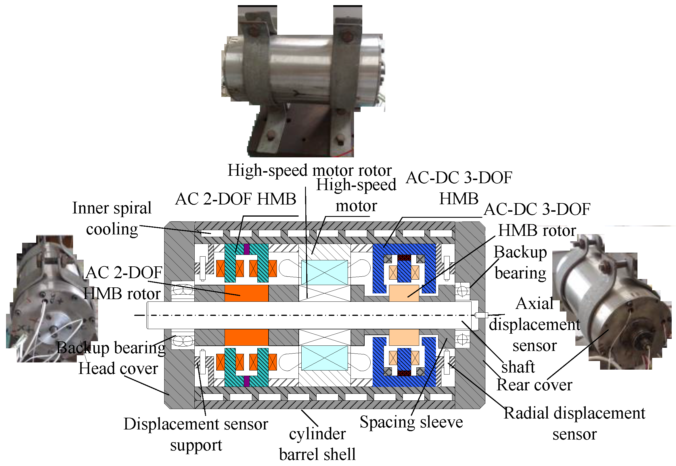
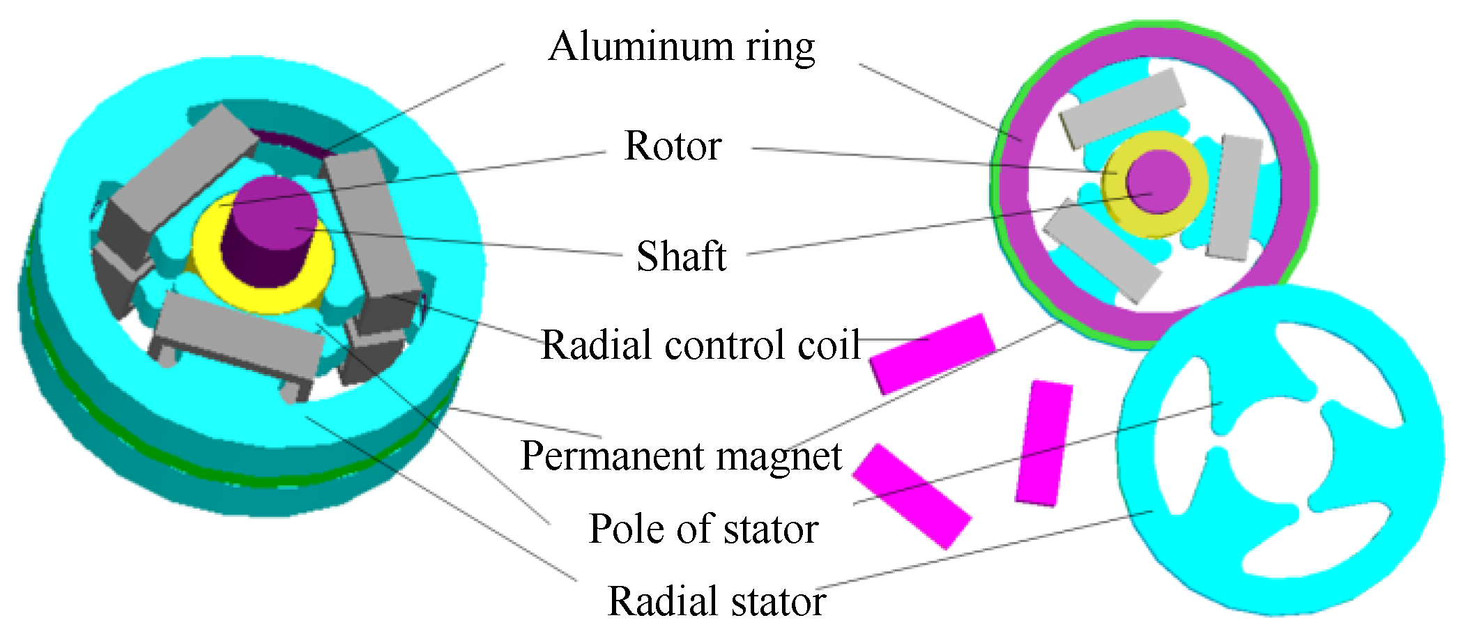
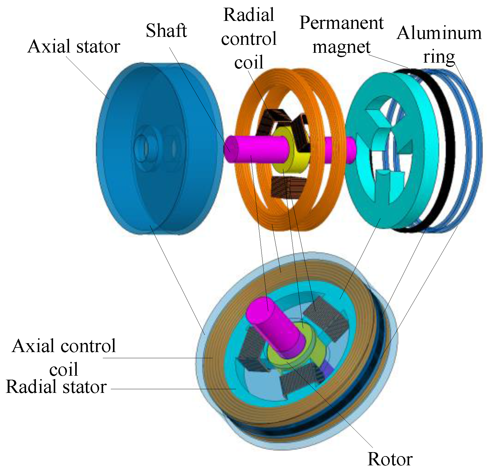
:1. Introduction
2. Generations of Mathematical Models
2.1. ClassicalFull Model
2.1.1. Classical Full Nonlinear Model
2.1.2. Classical Full Linear Model
2.2. Improved Full Model
2.2.1. Improved Full Nonlinear Model
2.2.2. Improved Full Linear Model
2.3. SwitchingFullModel
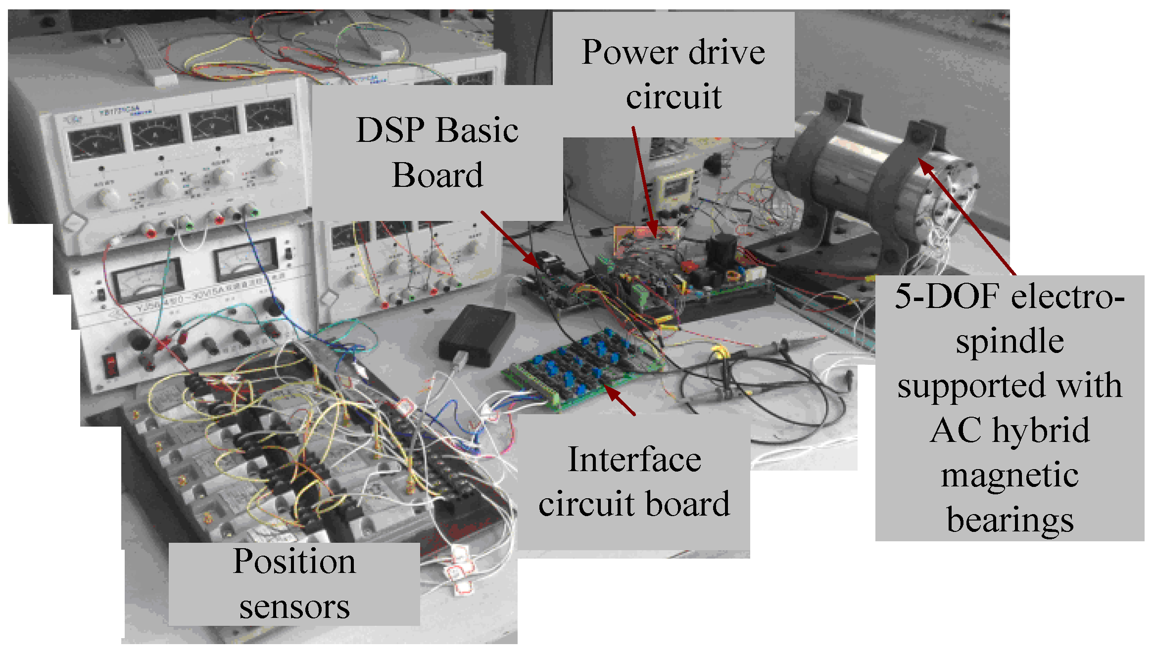
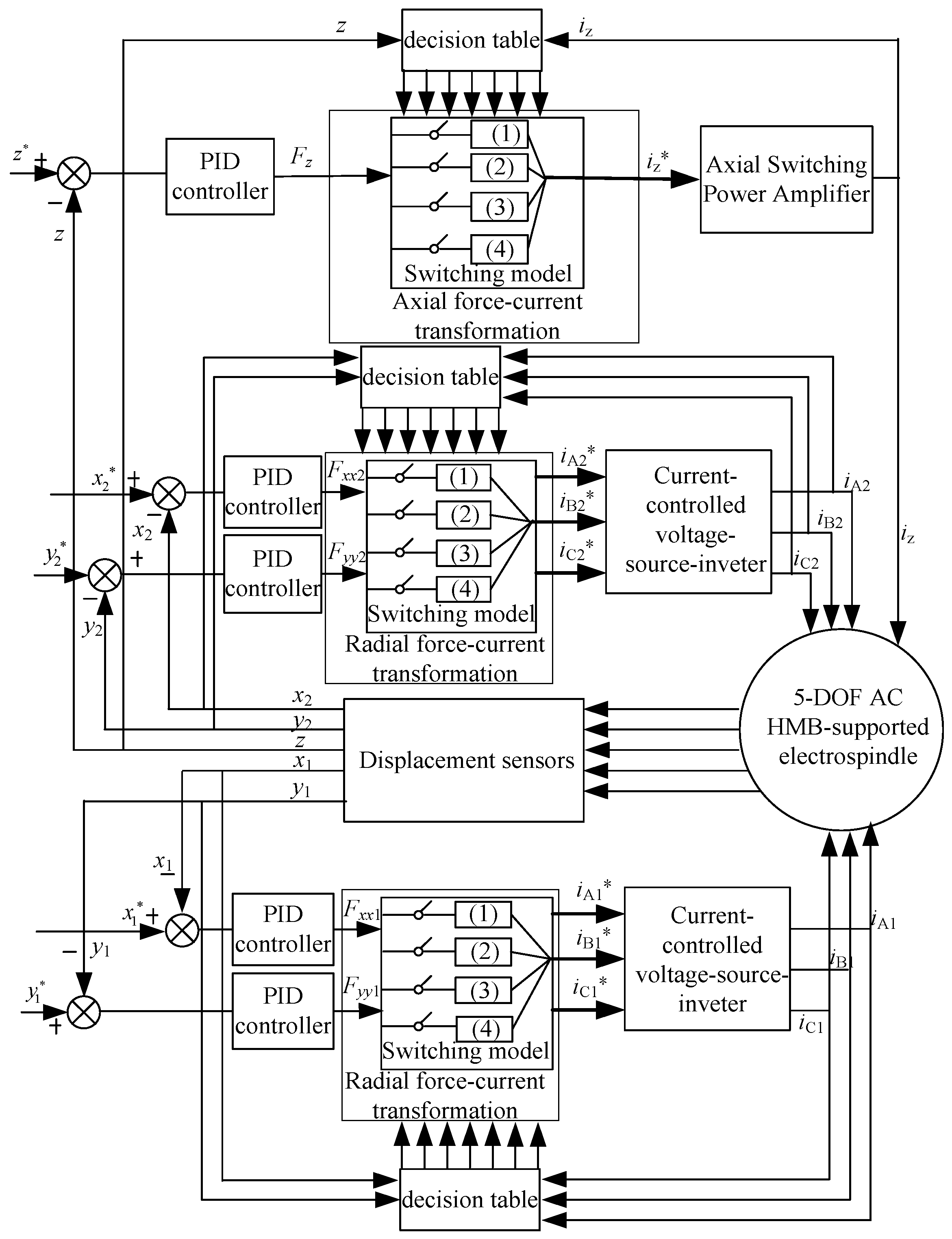
3. Switching Full Model Analysis Based on Experiments
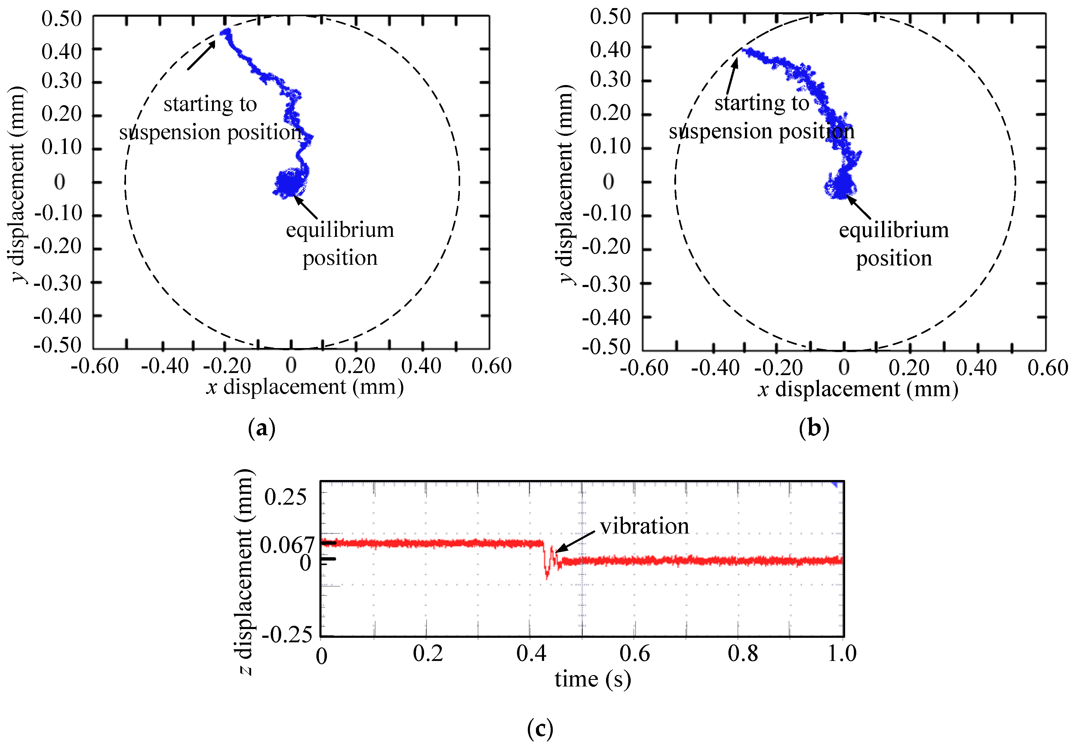
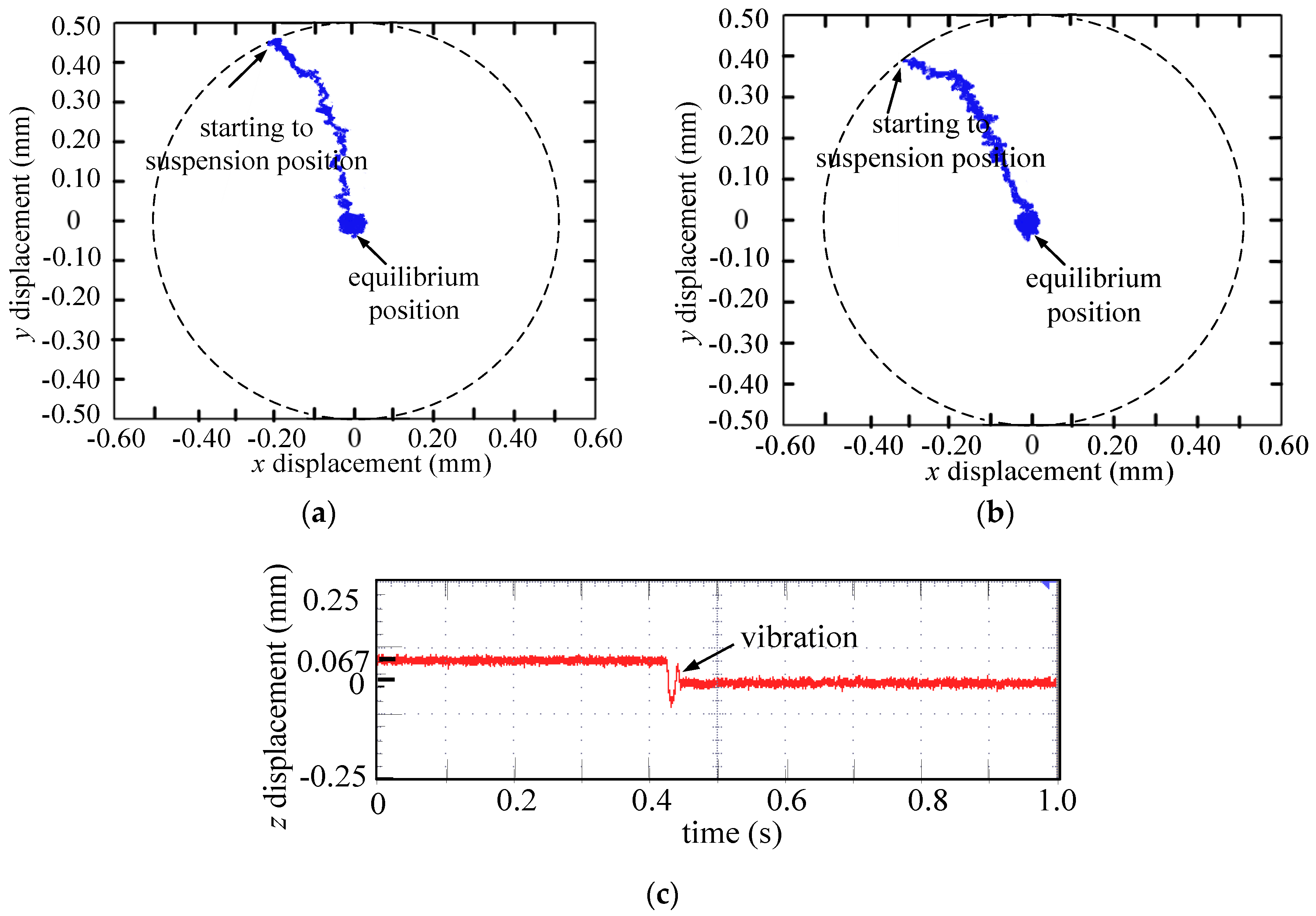
3.1. Start-of-Suspension Response Experiment
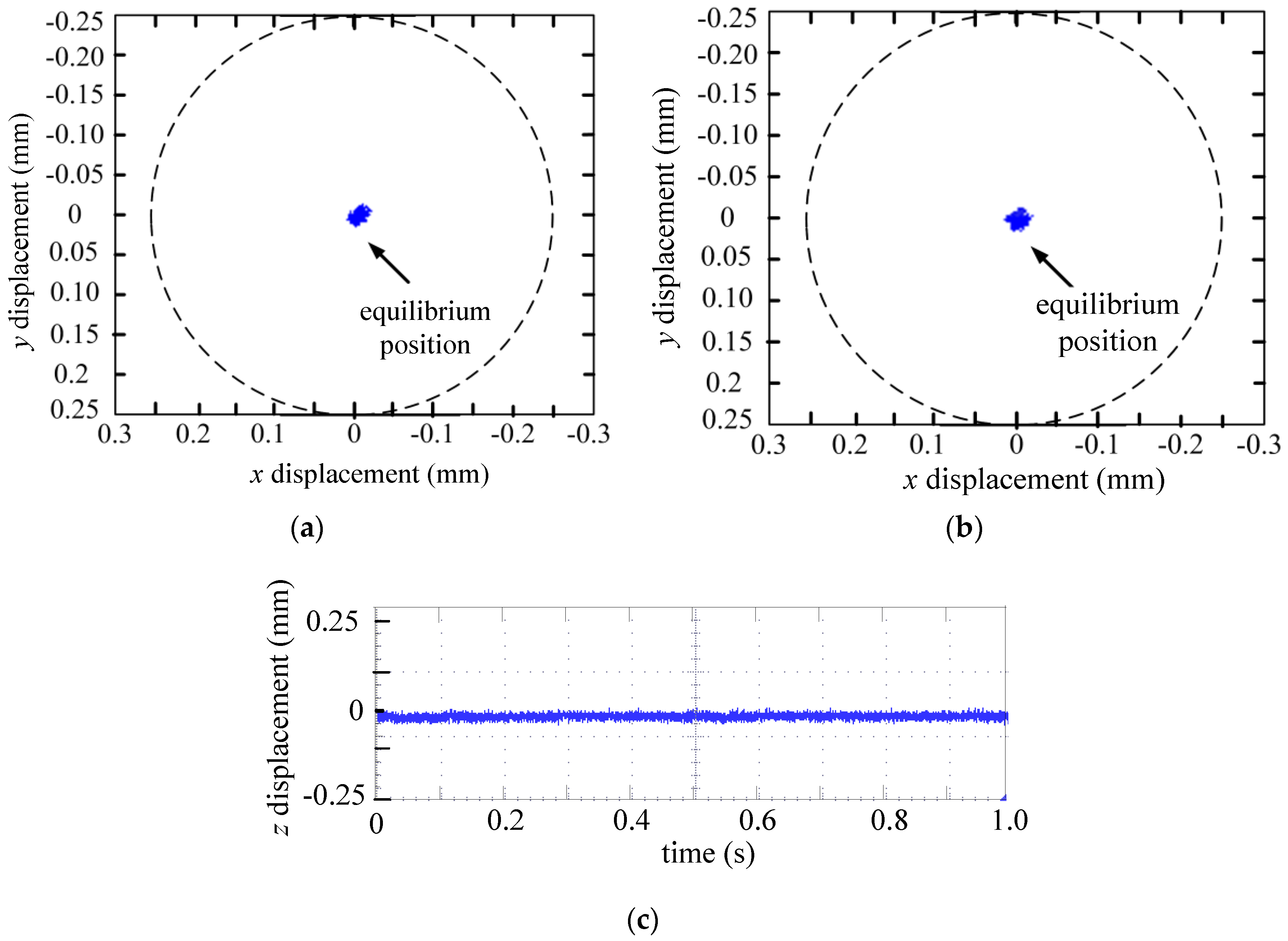
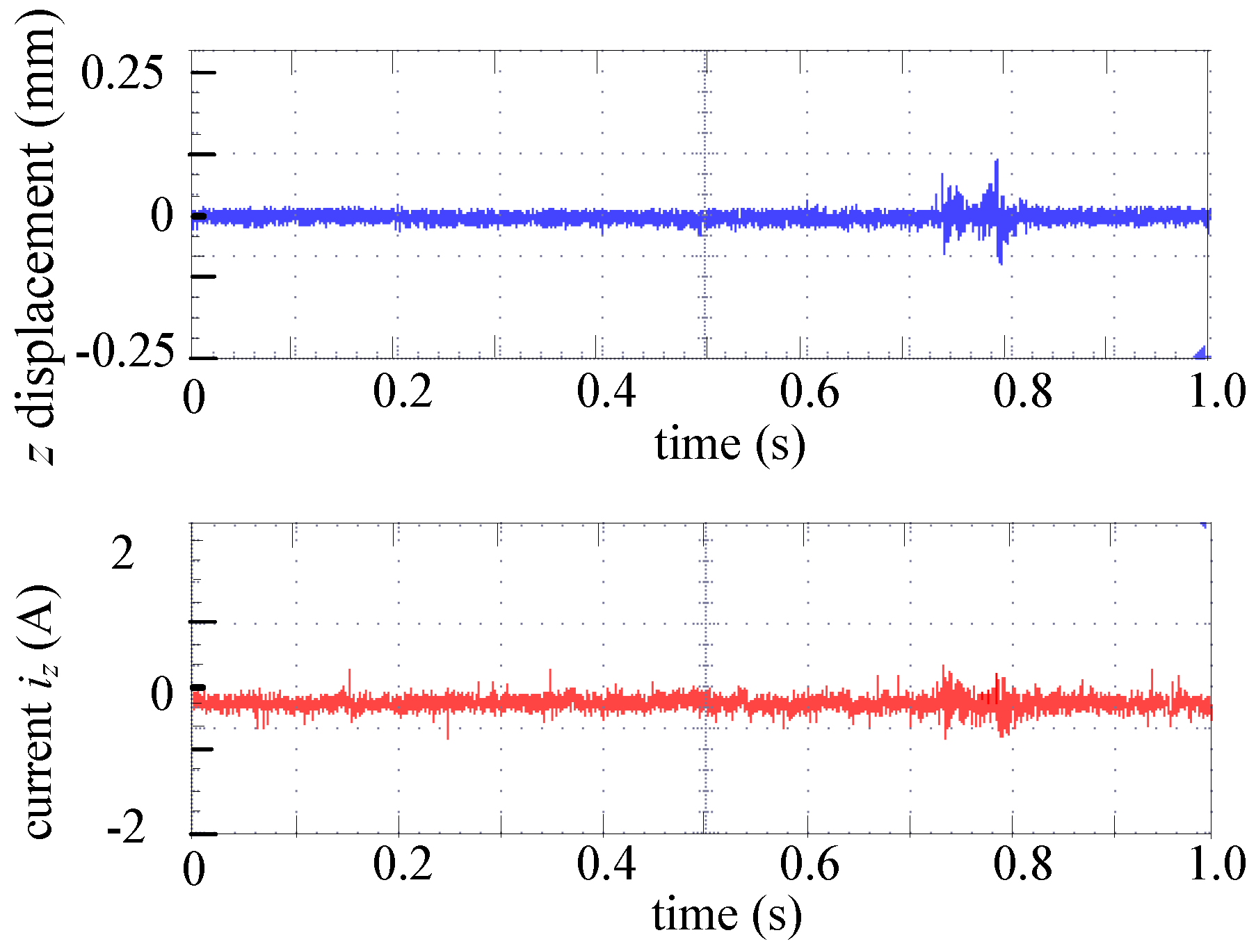
3.2. Suspension Experiment
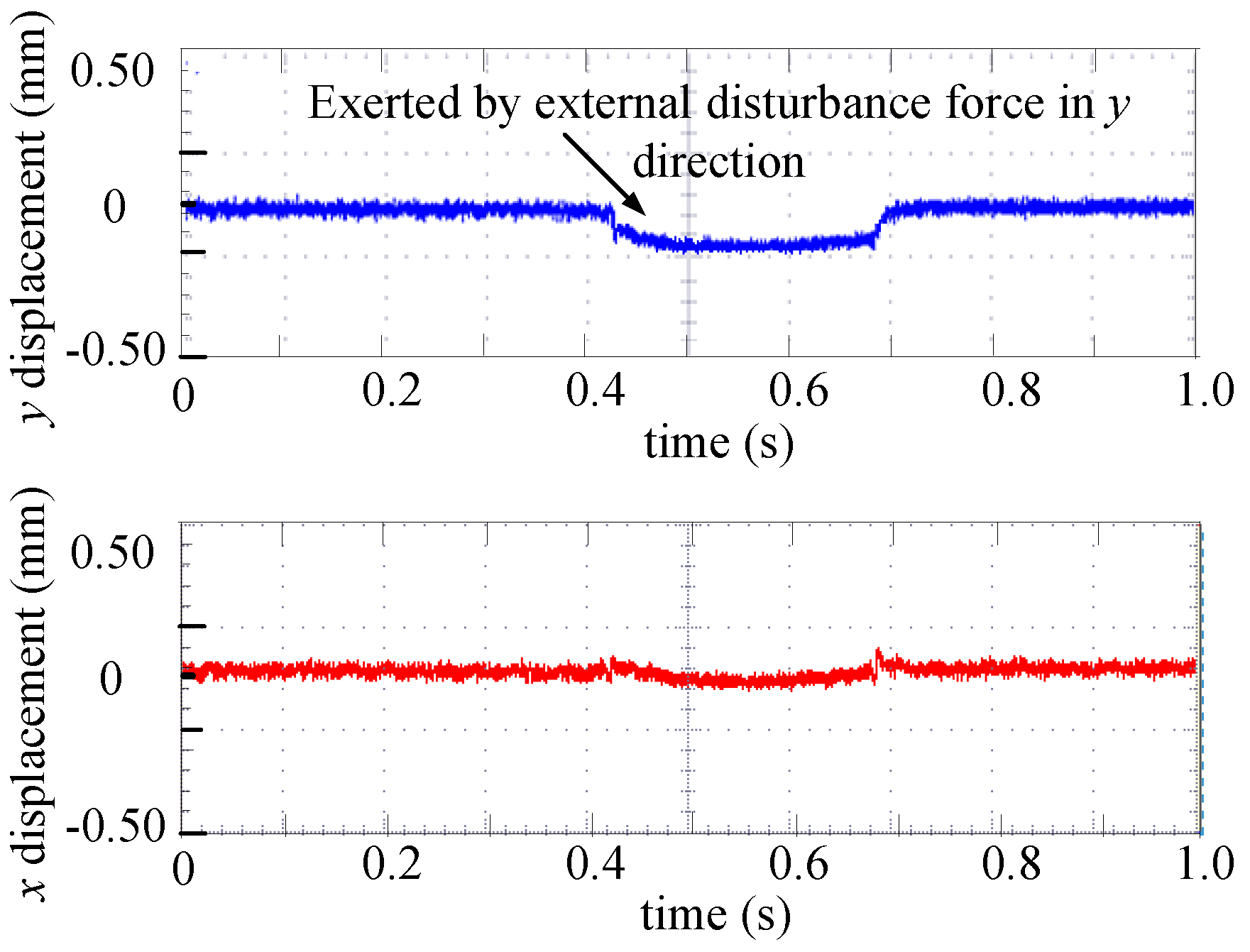
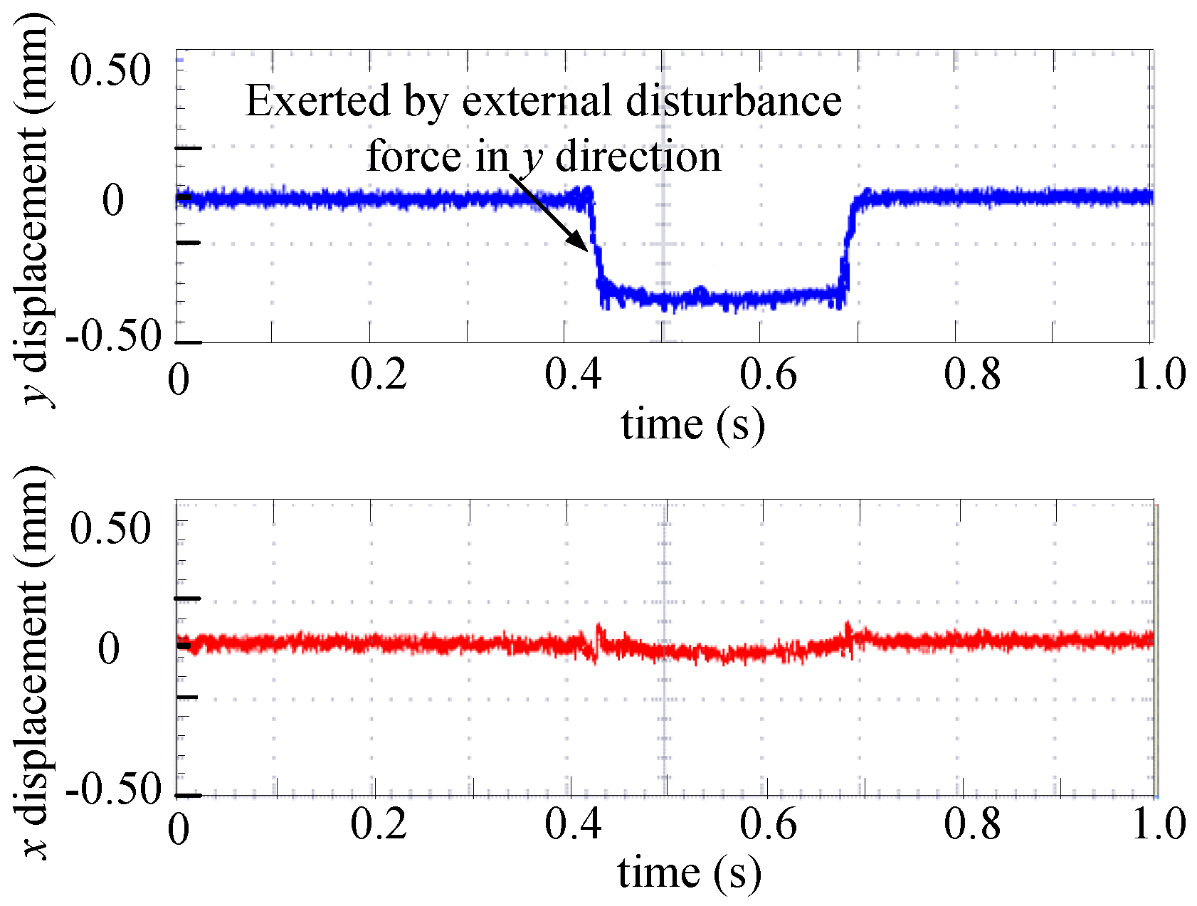
3.3. Disturbance Response Experiment
4. Full Prediction Model of Suspension Force according to Operating State
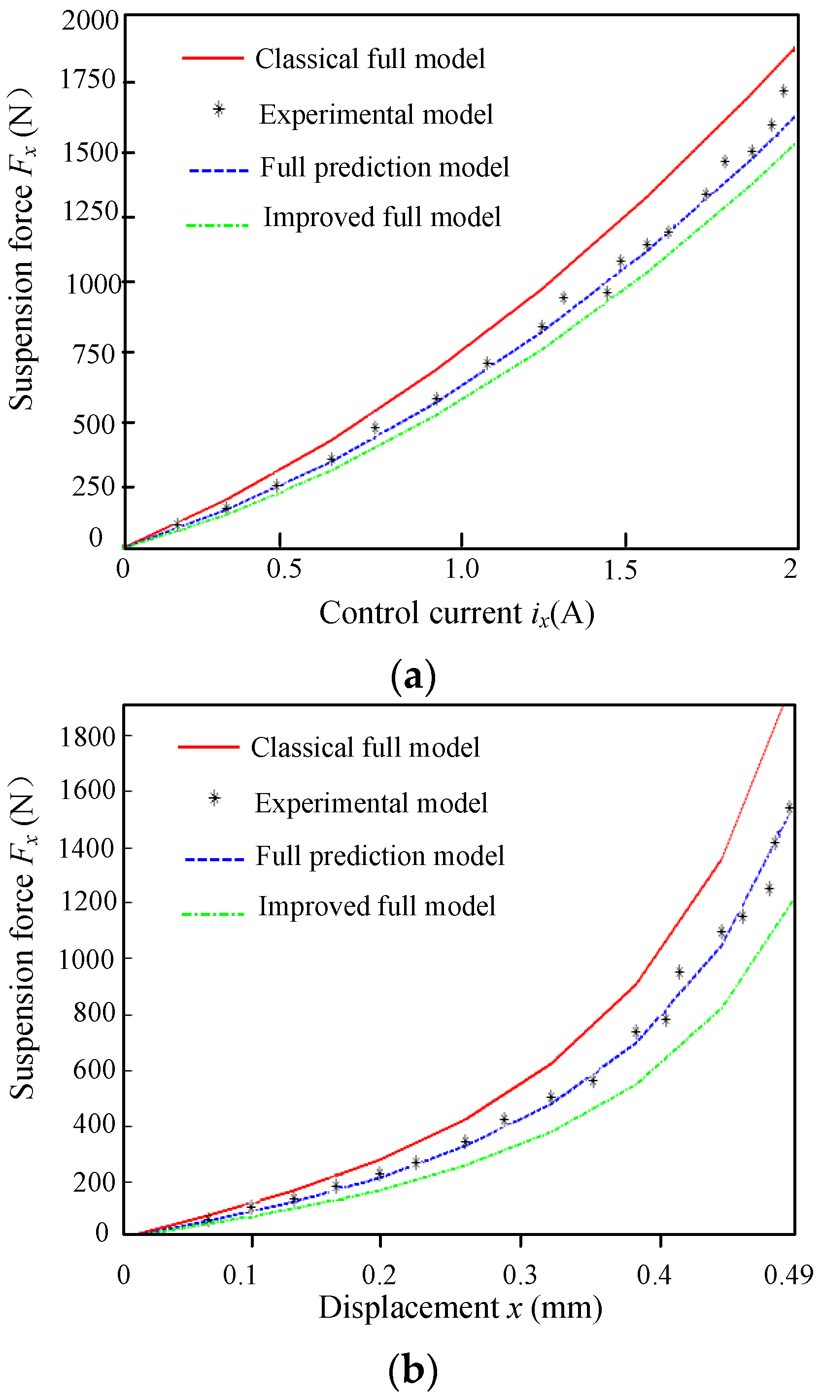
4.1. Comparative Experiment
4.2. Verification Experiment
4.3. Stiffness Tests and AccuracyAnalysis of the Model
5. Conclusions
Acknowledgments
Author Contributions
Conflicts of Interest
References
- Fang, J.C.; Zheng, S.Q.; Han, B.C. AMB vibration control for structural resonance of double-gimbal control moment gyro with high-speed magnetically suspended rotor. IEEE/ASME Trans. Mechatron. 2013, 18, 32–43. [Google Scholar] [CrossRef]
- Ren, Y.; Fang, J.C. High-stability and fast-response twisting motion control for the magnetically suspended rotor system in a control moment gyro. IEEE/ASME Trans. Mechatron. 2013, 18, 1625–1634. [Google Scholar] [CrossRef]
- Park, J.K.; Kyung, J.H.; Shin, W.C.; Ro, S.K. A magnetically suspended miniature spindle and its application for tool orbit control. Int. J. Precis. Eng. Manuf. 2012, 13, 1601–1607. [Google Scholar] [CrossRef]
- Pesch, A.H.; Smirnov, A.; Pyrhonen, O.; Sawicki, J.T. Magnetic bearing spindle tool tracking through-synthesis robust control. IEEE/ASME Trans. Mechatron. 2015, 20, 1448–1457. [Google Scholar] [CrossRef]
- Na, J.U. Fault tolerant homopolar magnetic bearings with flux invariant control. J. Mech. Sci. Technol. 2006, 20, 643–651. [Google Scholar] [CrossRef]
- Darbandi, S.M.; Behzad, M.; Salarieh, H.; Mehdigholi, H. Linear output feedback control of a three-pole magnetic bearing. IEEE/ASME Trans. Mechatron. 2014, 19, 1323–1330. [Google Scholar]
- Jv, J.T.; Zhu, H.Q. Radial force-current characteristics analysis of three-pole radial-axial hybrid magnetic bearings and their structure improvement. Energies 2016, 9, 706. [Google Scholar]
- Zhu, H.Q.; Ding, S.L.; Jv, J.T. Modeling for three-pole radial hybrid magnetic bearing considering edge effect. Energies 2016, 9, 345. [Google Scholar] [CrossRef]
- Schob, R.; Redemann, C.; Gempp, T. Radial active magnetic bearing for operation with a 3-phase power converter. In Proceedings of the 4th International Symposium Magnetic Suspension Technology, Gifu, Japan, 30 October–1 November 1997.
- Uhn, J.N. Design and analysis of a new permanent magnet biased integrated radial-axial magnetic bearing. Int. J. Precis. Eng. Manuf. 2012, 13, 133–136. [Google Scholar]
- Huang, L.; Zhao, G.Z.; Nian, H.; He, Y.K. Modeling and design of permanent magnet biased radial-axial magnetic bearing by extended circuit theory. In Proceedings of the International Conference on Electrical Machines and System, Seoul, Korea, 8–11 October 2007; pp. 1502–1507.
- Zhang, W.Y.; Yang, Z.B.; Zhu, H.Q. Principle and control of radial AC hybrid magnetic bearing. In Proceedings of the 12th International Symposium Magnetic Bearings, Wuhan, China, 22–25 August 2010; pp. 490–496.
- Zhang, W.Y.; Zhu, H.Q. Precision modeling method specifically for AC magnetic bearings. IEEE Trans. Magn. 2013, 49, 5543–5553. [Google Scholar] [CrossRef]
- Zhang, W.Y.; Ruan, Y.; Diao, X.Y.; Zhu, H.Q. Control system design for AC-DC three-degree-of-freedom hybrid magnetic bearing. Appl. Mech. Mater. 2012, 150, 144–147. [Google Scholar] [CrossRef]
- Zhang, W.Y.; Zhu, H.Q. Improved model and experiment for AC-DC three-degree of freedom hybrid magnetic bearing. IEEE Trans. Magn. 2013, 49, 5554–5565. [Google Scholar] [CrossRef]
- Zhang, W.Y.; Zhu, H.Q.; Yang, Z.B.; Sun, X.D.; Yuan, Y. Nonlinear model analysis and “switching model” of AC-DC three-degree of freedom hybrid magnetic bearing. IEEE/ASME Trans. Mechatron. 2016, 21, 1102–1115. [Google Scholar] [CrossRef]
- Zhang, W.Y.; Zhu, H.Q. Control system design for a five-degree-of-freedom electrospindle supported with AC hybrid magnetic bearings. IEEE/ASME Trans. Mechatron. 2015, 20, 2525–2537. [Google Scholar] [CrossRef]


| “Full operation-domain model” | Model | Equation | Current | Displacement | Multi-Zone |
| Model (1): Improved full nonlinear model | Equations (5) and (6) | 0–1 (A) & 1–1.5 (A) | 0–0.25 (mm) & 0.25–0.49 (mm) | Zone (1) | |
| Model (2): Classical full nonlinear model | Equations (1) and (2) | 1.5–2 (A) | 0.25–0.49(mm) | Zone (2) | |
Model (3):
|
| 1–1.5 (A) | 0.4–0.49 (mm) | Zone (3) | |
| Model (4): Classical full nonlinear model | Equations (1) and (2) | 1.5–2 (A) | 0.4–0.49 (mm) | Zone (4) |
| “Full prediction model” of suspension force according to operating state | Operating State | Initial Model | Position | Model Variation | Switching Point |
| start-of-suspension | Model (1) | Initial position: 0–0.25 (mm) | Changeless Model (1) | none | |
| Model (3) | Initial position: 0.25–0.44 (mm) | Model (3)→Model (1) | When the displacement enters into 0–0.25 (mm) | ||
| Model (4) | Initial position: 0.44–0.49 (mm) | Model (4)→Model (1) | When the displacement enters into 0–0.25 (mm) | ||
| suspension | Model (1) | Operating position: 0–0.25 (mm) | Changeless Model (1) | none | |
| Model (2) | Operating position: 0.25–0.49 (mm) | Model (2)→Model (1) | When the displacement enters into 0–0.25 (mm) | ||
| disturbed state | Model (1) | Maximum deviation postion: 0–0.25 (mm) | Changeless Model (1) | none | |
| Model (1) | Maximum deviation postion: 0.25–0.49 (mm) | Model (1)→Model (2–4)→Model (1) | When the displacement enters into 0–0.25 (mm), twice |
© 2017 by the authors; licensee MDPI, Basel, Switzerland. This article is an open access article distributed under the terms and conditions of the Creative Commons Attribution (CC-BY) license (http://creativecommons.org/licenses/by/4.0/).
Share and Cite
Zhang, W.; Zhu, H.; Yang, H.; Chen, T. Experimental Analysis and Full Prediction Model of a 5-DOF Motorized Spindle. Energies 2017, 10, 75. https://doi.org/10.3390/en10010075
Zhang W, Zhu H, Yang H, Chen T. Experimental Analysis and Full Prediction Model of a 5-DOF Motorized Spindle. Energies. 2017; 10(1):75. https://doi.org/10.3390/en10010075
Chicago/Turabian StyleZhang, Weiyu, Huangqiu Zhu, Hengkun Yang, and Tao Chen. 2017. "Experimental Analysis and Full Prediction Model of a 5-DOF Motorized Spindle" Energies 10, no. 1: 75. https://doi.org/10.3390/en10010075