
Robust Operation of Energy Storage System with Uncertain Load Profiles


Department of Electronic Engineering, Sogang University, 35 Baekbeom-ro, Mapo-gu, Seoul 121-742, Korea
*
Author to whom correspondence should be addressed.
Energies 2017, 10(4), 416; https://doi.org/10.3390/en10040416
Submission received: 31 December 2016
/
Revised: 2 March 2017
/
Accepted: 18 March 2017
/
Published: 23 March 2017
(This article belongs to the Special Issue Industrial Energy Efficiency)
Abstract
:In this paper, we propose novel techniques to reduce total cost and peak load of factories from a customer point of view. We control energy storage system (ESS) to minimize the total electricity bill under the Korea commercial and industrial (KCI) tariff, which both considers peak load and time of use (ToU). Under the KCI tariff, the average peak load, which is the maximum among all average power consumptions measured every 15 min for the past 12 months, determines the monthly base cost, and thus peak load control is extremely critical. We aim to leverage ESS for both peak load reduction based on load prediction as well as energy arbitrage exploiting ToU. However, load prediction inevitably has uncertainty, which makes ESS operation challenging with KCI tariff. To tackle it, we apply robust optimization to minimize risk in a real environment. Our approach significantly reduces the peak load by 49.9% and the total cost by 10.8% compared to the case that does not consider load uncertainty. In doing this we also consider battery degradation cost and validate the practical use of the proposed techniques.
1. Introduction
The energy storage system (ESS) has become popular in recent times due to the proliferation of intermittent renewable energies such as wind and solar power [1]. Furthermore, battery prices have been falling notably in recent years, and this enables consumers to have their own ESS to reduce electricity bill with the development of low cost energy storage devices [2]. By using ESS, users can charge electrical energy when electricity price is low and discharge the energy in ESS when electricity price is high. From social welfare point of view, installing ESS is also encouraged because it is possible to reduce peak load and resolve overload problems threatening operational reliability in a distribution network [3]. In this regard there have been many efforts to minimize electricity bill by using ESS [4,5,6,7,8].
In most countries, electricity price is determined by time of use (ToU), critical peak pricing or real time pricing [9]. Among various electricity price policies which differ from countries to countries, we specifically consider the case of Korea where electricity bill for industrial customers is calculated based on both monthly peak load and daily ToU tariff. Note that the way of peak load charging in Korea is very unique compared to other countries. Roughly speaking, the monthly base electricity cost is determined by the highest power consumption out of all average power consumptions measured every 15 min for the past one year including the month of consideration. This implies that peak load without control, even only for 15 min, may affect the monthly base cost for 12 months. Thus, unlike the U.K. triad period where customers need to reduce the load during the predetermined three half hour periods, Korea’s peak load charging requires customers to minimize the 15 min-peak load at any moment. Hence, commercial and industrial customers should be extremely careful to reduce their peak load during summer and winter. Under this unique tariff, using ESS is promising, and there was an attempt to use demand side management and ESS to minimize total cost [10].
In operating ESS, load forecasting is essential for both peak load reduction and energy arbitrage exploiting ToU. Load forecasting, however, cannot be always accurate since it is related with unexpected exogenous inputs for operations as well as weather conditions [11]. Nevertheless, many previous works about ESS operation did not actively consider load uncertainty [12,13,14]. In this regard, we leverage robust optimization for ESS scheduling to solve the problem of load uncertainty. In doing this, we further consider battery wear-out cost to compute the realistic operational cost as well as the proper capacity of ESS.
We summarize our contributions as follows. First, we provide a framework for industrial customers in Korea to minimize the total cost considering peak load pricing and ToU. Under the Korea commercial and industrial (KCI) tariff, ESS operates to minimize peak load in a month as well as ToU cost in a day. Second, we propose robust optimization algorithms for total cost minimization in a realistic environment. There are several risks that may occur when load uncertainty is not considered; specifically under KCI tariff, unmanaged peak load in a month may determine the base electricity cost for up-to one year. We apply robust optimization to set robust margin considering the distribution of prediction errors. Our results show that both total cost and peak load are reduced significantly by 10.8% and 49.9% respectively compared to the case of deterministic optimization that does not consider load uncertainty. Third, our approach considers battery wear-out cost to provide accurate cost comparison, and simulates different battery capacities to determine appropriate battery size that minimizes total cost in industry.
The remainder of the paper is organized as follows. We present a framework of robust ESS operation in Section 2 where we formulate an optimization problem to obtain the ESS charging and discharging strategy, and describe a way to minimize the risk with uncertain load profile. Case study results along with electricity bill and battery wear-out cost are described in Section 3 to analyze the performance of our algorithms as well as to suggest proper battery capacity and robust proportion. Then, we conclude our paper in Section 4.
2. Robust ESS Operation Framework
In this section we provide a framework for robust ESS operation for daily as well as for year-round operation. We consider a system model for smart grid environment where ESS is installed in a customer’s premise such as factory. Load profiles vary depending on the characteristics of industries, and we select a car manufacturing factory as a typical example. However, our method can be easily applicable to other types of industries.
2.1. System Model
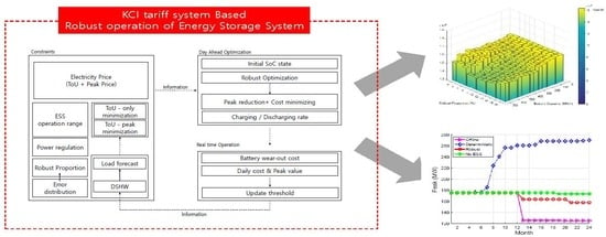
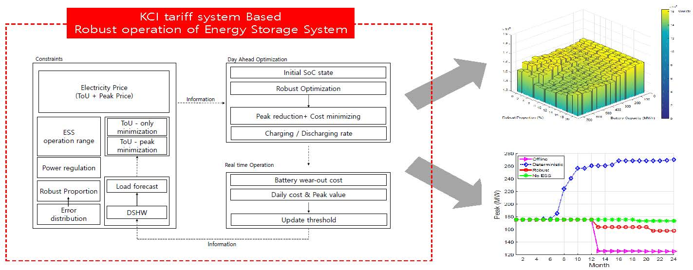
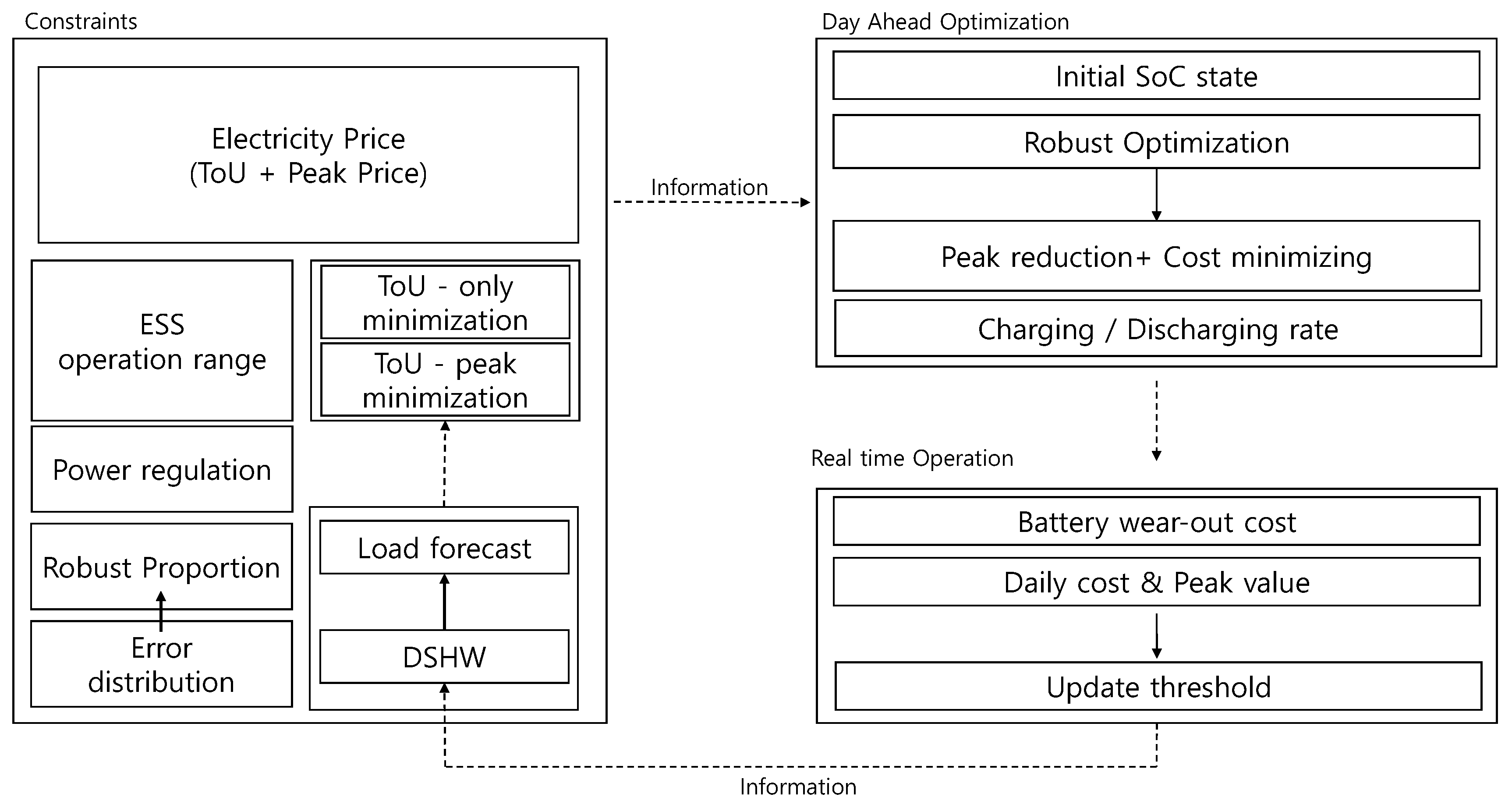
Figure 1 shows the overall structure of a robust ESS operation. Our model is specifically focused on the case of Korea commercial and industry customers, so both peak pricing and ToU are considered. Note that we have two different operational modes; ToU-only-minimization is performed when the expected peak load of the day is less than the historical peak load for the past one year. ToU-peak-minimization is performed when the monthly peak is expected to occur during the day. Such decision is based on short-term load forecasting. Even though our framework is independent of short-term load forecasting techniques, we use the double seasonal Holt–Winters (DSHW) [15], which is one of the popular time series load forecasting techniques. Note that, however, our method is compliant with any kind of load forecasting methods such as the newly developed deep neural network (DNN)-based model [16,17]. Then, we compute the error distribution between predicted and real load profiles, which is used to set robust margin, or called robust proportion hereafter. In operating ESS, state of charge (SoC) has its own recommended operational range. Sometimes, in addition, there is regional power regulation in using ESS; for example, power injection from ESS to the grid is yet allowed in Korea. Based on the constraints mentioned so far, robust optimization is performed, and ESS charging and discharging rates are computed. Finally, based on the realized load profile and ESS operation, the historical peak value is updated, and daily operational cost is computed in addition to computing realistic battery degradation cost using battery wear-out model [18].
2.2. Load Uncertainty
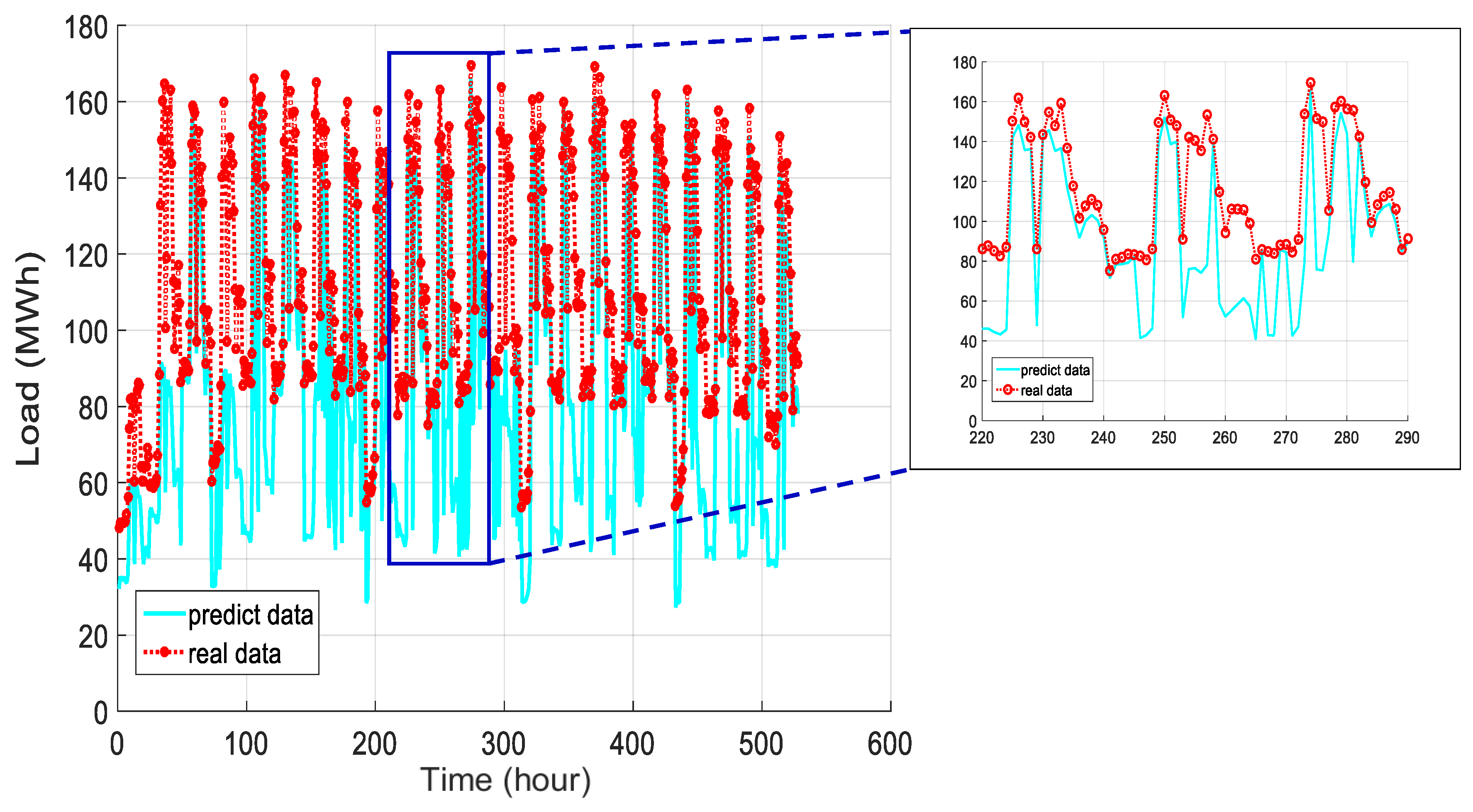
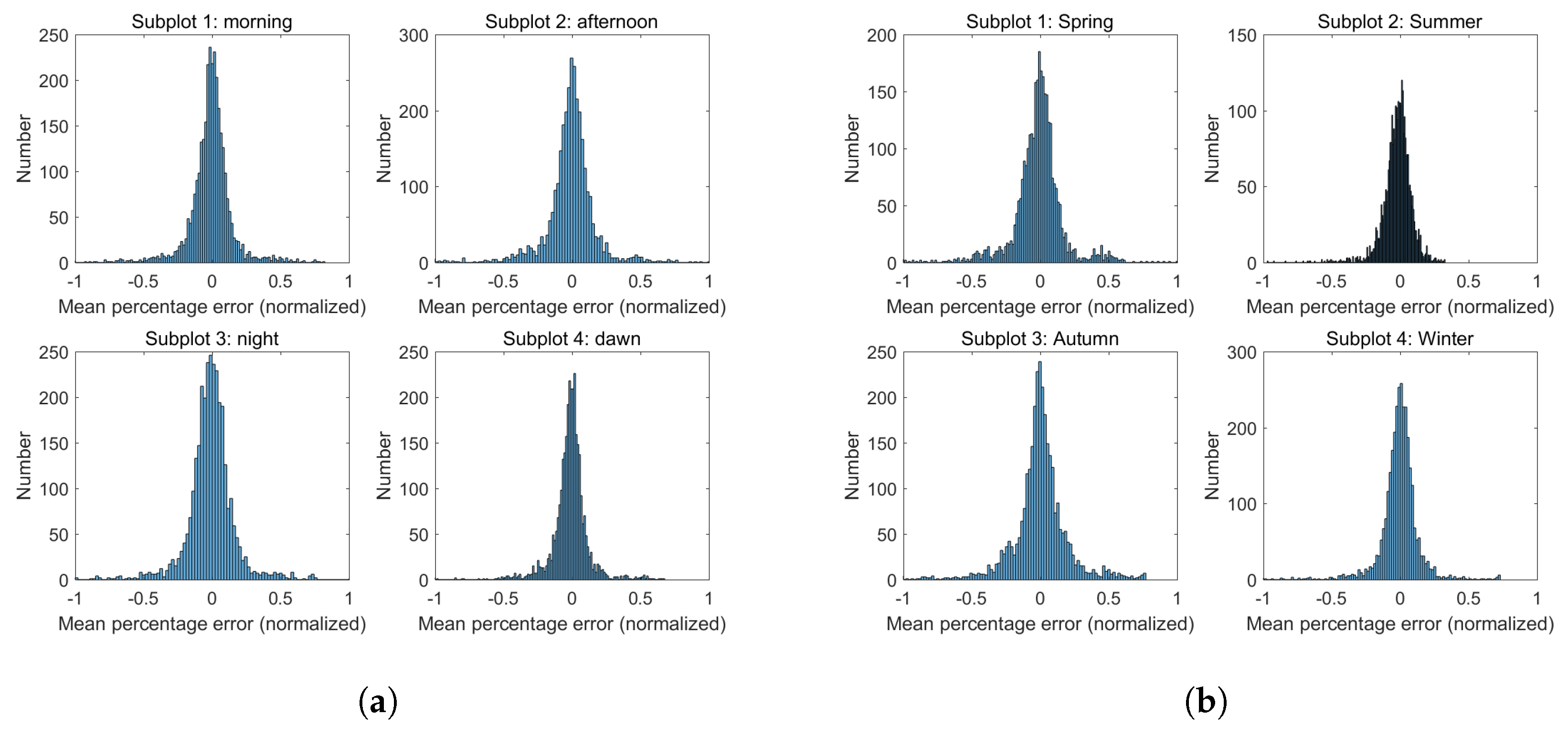
As we discussed, accurate load forecasting is essential to operate ESS, but load uncertainty inevitably exists, which depends on the type of loads, the time of day, the season of year, etc. To illustrate this we provide Figure 2a as an example of real load profile and its prediction based on DSHW [15,16]. For illustrative purpose, the unit of x-axis is chosen to be one hour. To further investigate the error distributions, we provide the distribution of mean percentage error (MPE) during a day in Figure 3a. As can be seen, errors are not negligible at all, i.e., normally a few tens of percent error exist in the morning, afternoon, night and dawn. We also check the error distributions for spring, summer, fall and winter and observe in Figure 3b that there are seasonal variations as well. These error distributions will be used to determine robust proportion to minimize risk in Section 3.3. Not that, in Figure 2, the prediction algorithm underestimates the real load for most of the time. In fact, we observe that the errors in each hour are not independent, and DSHW sometimes overestimates and sometimes underestimates for almost a whole day. However, as shown in Figure 3, when the MPE distribution is obtained for a long period of time (e.g., two years), the average of MPE is almost zero, i.e., the occurrences of overestimation and underestimation are almost same.
2.3. Daily Operation of ESS with Uncertain Load Profile
In this section we derive charging/discharging rate and the desired SoC in each time slot in a daily operation with uncertain load profile. This result will be extended to year-round operation in Section 2.4 Let denote a realized load profile of a typical day, which is a T dimensional vector, i.e., there are T time slots in a day,
Let denote the predicted load profile of ,
Let denote a normalized charging/discharging schedule vector, of which element lies on and will be obtained by optimization process.
Let . In battery operation, means battery charging and means battery discharging, . For practical operation, the SoC of battery must be within some range, i.e., between and . So we have the following constraint,
where is the initial battery state, and r is the maximum charging/discharging rate of ESS. Since the regulation in Korea currently prohibits from reselling extra energy of ESS to the grid, we have an additional constraint:
We further assume that SoC level at the beginning of each day is identical. Thus, the summation of charging and discharging rates over one day should be zero,
For notational simplicity, we define as a feasible set of that satisfies (4)–(6). Recall that the electricity bill of Korea industry has two parts: base cost that is determined by peak load of a month, and ToU cost. Thus, we consider both peak reduction and ToU pricing in our objective function and formulate linear programming as follows,
Problem 1:
where represents the ToU price at time slot i and is a weight factor to reflect the importance of base cost vs ToU cost. Since it is hard to solve min/max problem using linear programming, we transform (7) into an equivalent problem by using an auxiliary variable as follows.
Problem 2:
Problem 2 is linear programming that reflects a way to reduce peak load. As a result, ESS operates to minimize the total cost considering both the peak load and ToU. Note that the formulation (2)–(9) is valid only if all parameters are known in advance (or called determined hereafter). However, load profile needs to be predicted and thus is subject to uncertainty.
Now, under load uncertainty we exploit robust optimization for conservative operation. In order to develop robust ESS operation algorithm, we first introduce the robust optimization derived from the following nominal linear programming [19].
Robust Optimization:
where is a transpose of a cost vector , is a matrix, of which elements may have uncertainty, is a constraint vector, which will be defined later and is an all one vector. To apply robust optimization, we transform Problem 2 into the above formulation of (10)–(12). Since in (5) and (9) is uncertain, we put (5) and (9) into the following equivalent matrix form as in (13):
Note that (13) has the same structure of (11) except that is augmented by 1 to be associated with the uncertain load profile. Consequently, uncertainty only exists at column of . Now we apply the robust optimization in [19], which boils down to the Soyster’s method in our case [20] such as:
Problem 3:
where is a by matrix from (11) and (13), , and is a set of j with uncertain at ith row. It is assumed in [20] that, for , lies in the interval where serves as the uncertainty boundary of . We see that uncertainty only arises at column of because uncertainty comes from the forecasted load data in (5) and (9). When is an optimal solution of Problem 3, then [20], and thus (15) becomes:
Note that for and should be determined by analyzing historical load profiles and their prediction errors as presented in Section 2.2
Example 1 (Robust optimization).
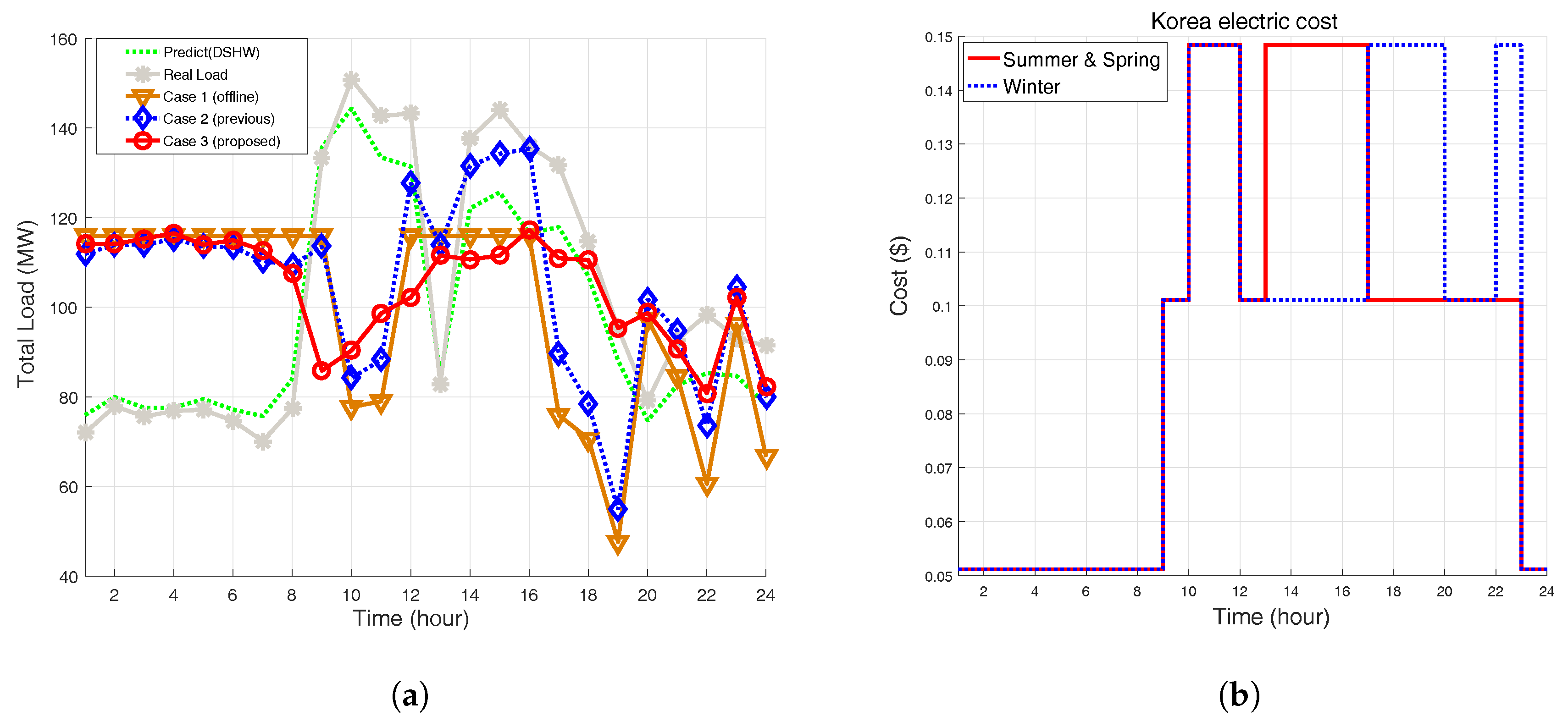
Before extending our work to year-round robust ESS operation in Section 2.4, we compare the daily results using different optimization methods in Figure 4a. Simulations parameters are same as in Section 3. As can be seen, if there were no uncertainty in load forecasting, it would have been possible to minimize peak load by 118 MW as shown in Case 1. We call it offline optimization because ESS scheduler perfectly knows the future. However, the real load during 9 AM–12 PM and 14 PM–17 PM is higher than the predicted load, which results in the peak load 138 MW as shown in Case 2. We call it deterministic optimization because ESS scheduler does not consider load uncertainty but operates in a deterministic way. To minimize risk under load uncertainty, robust proportions are set; we will discuss how to determine robust proportion in Section 3.3. As a result, robust optimization in Case 3 sustains the peak load by 119 MW, which is lower than that of deterministic case. Since the monthly base cost is determined by peak load multiplied by $8.3/kW, the customer saves more than $166,000 in a month. Note that the charging/discharging schedule of Case 3 is the result of robust optimization, which both considers ToU and peak minimization under uncertainty. As shown in Figure 4b, ToU is the lowest during 0–8 AM, so ESS charging is mostly done during that time. Interestingly, by using ESS, the load during 0–8 AM, which was the valley of the daily load pattern, becomes same to the daily peak load at 4 PM.
2.4. Year-Round Operation of ESS with Uncertain Load Profile
Based on the daily operation of ESS with uncertain load profile, we now extend it to year-round operation. Note that year-round operation is not simply the repetition of the daily operation because of the unique KCI tariff. Indeed it becomes more challenging with load uncertainty recalling that unmanaged peak load, even only for 15 min, may affect the base costs of the 12 months. Under this circumstance, to be practically applicable to industry customers, we further develop a year-round robust ESS operation algorithm as shown in Figure 5.
Let n be a day index and m be a month index. Let and denote the realized load profile and the charging/discharging rate of day n at time slot i, respectively. Then, the daily peak load is denoted by , and the monthly peak load is denoted by where is a set of working days of month m. Let denote the historical peak load from the past 12 months excluding spring and fall (which is denoted by ), and up to the day n of month m. Then, we have:
Let denote day-ahead peak load estimation of day n of month m. Then, based on , ESS determines whether to control peak load or not. If the estimated peak load is less than the historical peak , passive peak load control is performed; ESS operates just to minimize the ToU cost with the peak load constrain of . The term `passive’ implies that peak control is not in the objective function but only in the constraint (case: No in the flowchart). By contrast, if a new peak is likely to occur tomorrow, ESS operates to jointly minimize peak load as well as ToU cost in the objective function at the same time (case: Yes). The subtlety lies in that, if the realized load happens to be a lot higher than the expected value , the peak load may exceed even though it could have been kept lower than .
In order to avoid this subtle case, we conservatively design the algorithm by discounting by so that peak load control can be done more often. is then updated everyday as in (22). Let be the ToU cost of day n of month m, which is simply given by:
When n reaches the end of the month, the monthly electricity bill, which is the sum of base cost and the ToU cost is computed by:
Finally, after year-round operation, the yearly cost is computed.
3. Simulation Results
In this section, we present the simulation results based on the proposed algorithms. We compare the result based on four representative cases and analyze the performances in terms of total cost minimization and peak reduction under different experimental environments.
3.1. Experimental Set-Up
The load profile is predicted by DSHW algorithm using past two weeks of data. Based on the prediction error distribution obtained in the past, we set the robust proportion, which was explained in Section 2.1. The average power consumption is measured every 15 min so is the operational decision of ESS charging/discharging.
Figure 6 represents the load profile of the car factory which is used in whole of simulation results in Section 3. In the load profile, we see repetitive load patterns which have specific peak values that make it appropriate to use ESS in KCI tariff system.
Table 1 summarizes the simulation parameters. The unmanaged peak load is more than 150 MW, the capacity of ESS is 400 MWh, and charging/discharging efficiency of ESS is 90%. Battery operating SoC range is set between 10%–90% because battery degradation is severe when SoC level is below 10% or higher than 90% as depicted in [21]. In calculating the cost, we do not include the cost of air conditioners that is required to keep the ESS room temperature moderate assuming that customers’ load is dominant so the load of air conditioners is negligible. Weighting factor is the inverse of base electricity price. We use battery price quoted from the practical data [22], and the battery price per kWh is $150, and total cycle life is about 3500 cycles when battery is used with 80% depth of discharge (DoD).
3.2. Case 1: Comparison of Peak Reduction
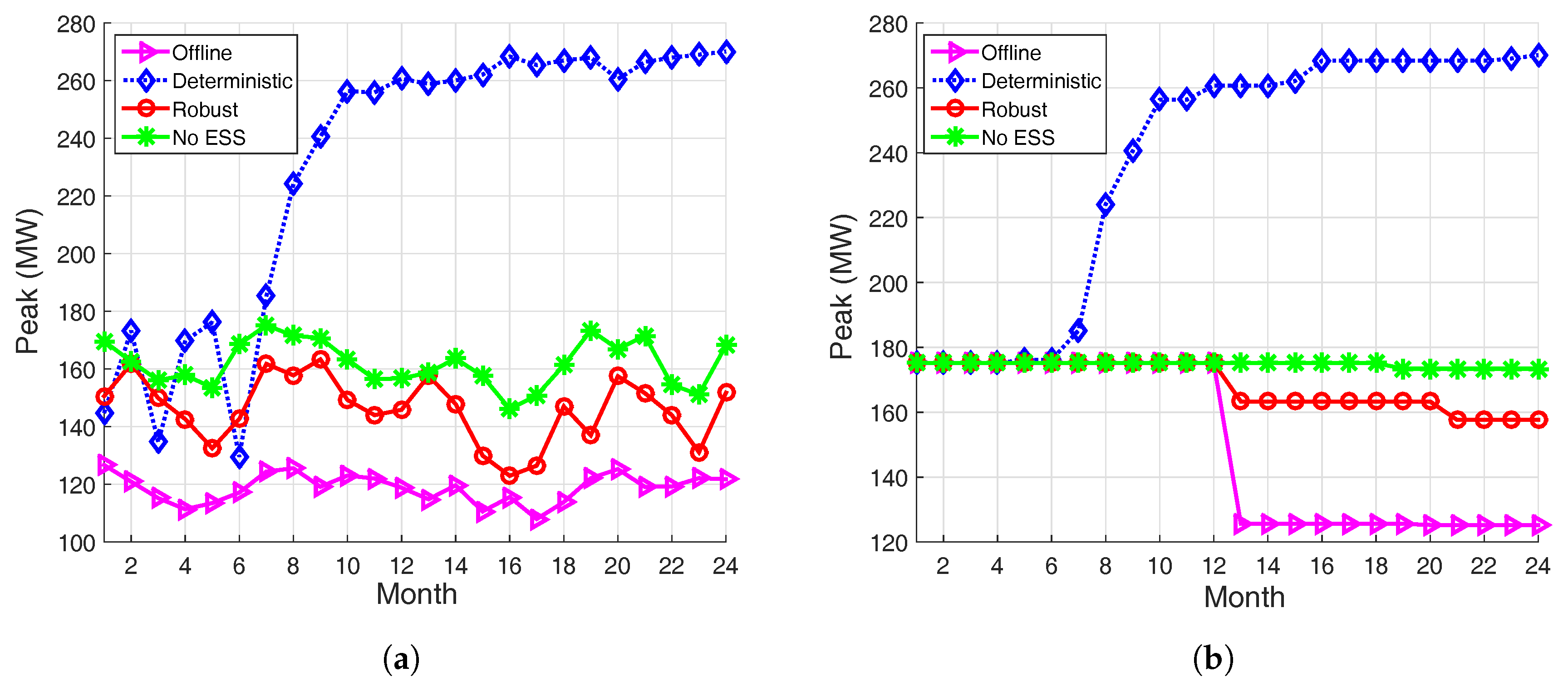
In this section, we show how appropriate robust optimization is to reduce peak load in a real situation. Figure 7a shows the monthly peak loads for two years in four different cases: offline, deterministic optimization, robust optimization and no ESS. In the case of offline, we assume that the optimizer perfectly knows the future. Offline case achieves the best result and is provided to compare the results of other algorithms. Deterministic optimization is the case when the algorithm solely relies on predicted data in a deterministically, i.e., does not consider load uncertainty. Thus, deterministic optimization can be vulnerable to prediction errors as we will see shortly. Robust optimization is the case when load prediction uncertainty is considered. No ESS is the case when ESS is not installed and thus serves as a baseline. As can be seen in Figure 7a, the monthly peak loads obtained from year-round robust operation are between no ESS and offline cases. Interestingly, however, the deterministic case is sometimes even worse than no ESS case because it is vulnerable to prediction error; when the peak load is wrongly managed due to load prediction error from August to October, the historical peak load keeps excessively high, which discourages the peak load control in the subsequent 11 months. We call it the memory effect due to the failure of peak load control.
Figure 7b shows the historical peak load, which determines the base price of each month and may last for the subsequent 11 months. It is interesting to observe that even in the offline case, the historical peak load remains around 170 MW for up-to one year. This is due to the peak load of December in the previous year (which is not shown in the figure), before the proposed algorithm is applied. This implies that it takes one year to see the effect of installing ESS and peak load control. However, the historical peak values finally decrease in the second year for the case of offline and robust optimization. By contrast, we see that deterministic optimization suffers from unexpectedly high peak load, and even worse than no ESS case.
3.3. Case 2: Monte Carlo Simulation to Determine Proper Robust Proportion
Before applying the proposed algorithm into real data, we discuss how to determine robust proportion, in (15) by analyzing the distribution of prediction errors. As shown in Figure 8, the error distribution of follows normal distribution with and (i.e., almost zero mean and around 10% of error in average). To observe the effect of prediction error distribution on peak load and to derive proper robust proportion, we perform a Monte Carlo simulation by generating a large set of load profiles that are deviated from the load prediction with varying from 0 to 0.2.
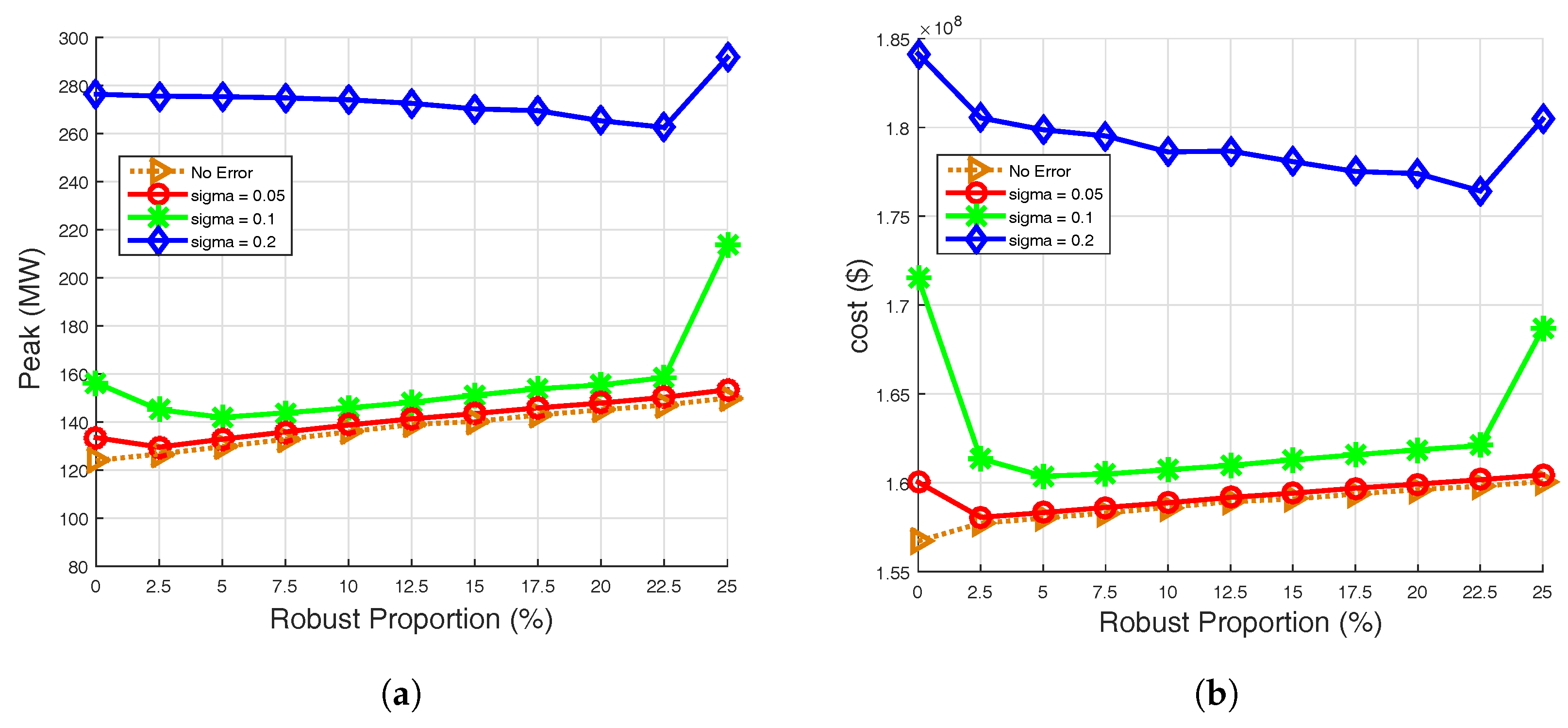
Figure 9 shows the result of peak value and electricity bill for various robust proportions and . We focus on peak value because it affects electricity bill for up-to one year. In Figure 9a, we see that robust proportion that minimizes peak load increases as grows. Furthermore, excessive robust proportion is not beneficial at all. This is because unnecessarily conservative operation makes become high. It is interesting to see that the peak values are not sensitive to the choice of robust proportion. The property of insensitivity is desirable in real operation because exact error distribution is hard to know in advance. Based on the observation in Figure 9a we set the robust proportion as 10% for operation with real data in the subsequent section. Figure 9b shows the electricity bill, which is the sum of peak cost and ToU cost. Even though electricity bill is insensitive to robust proportion, there are severe undesirable results when robust proportion is too small or too high, e.g., below than 2.5% or higher than 22.5%. This is because when the proportion is set below than 2.5%, there is not enough consideration of uncertainty to minimize peak load and cost. In addition, it is hard to reduce peak load if we set robust proportion too high because some portion of ESS is not utilized at all. This is also observable when is zero.
3.4. Case 3: Cost Comparison for Year-Round Operation
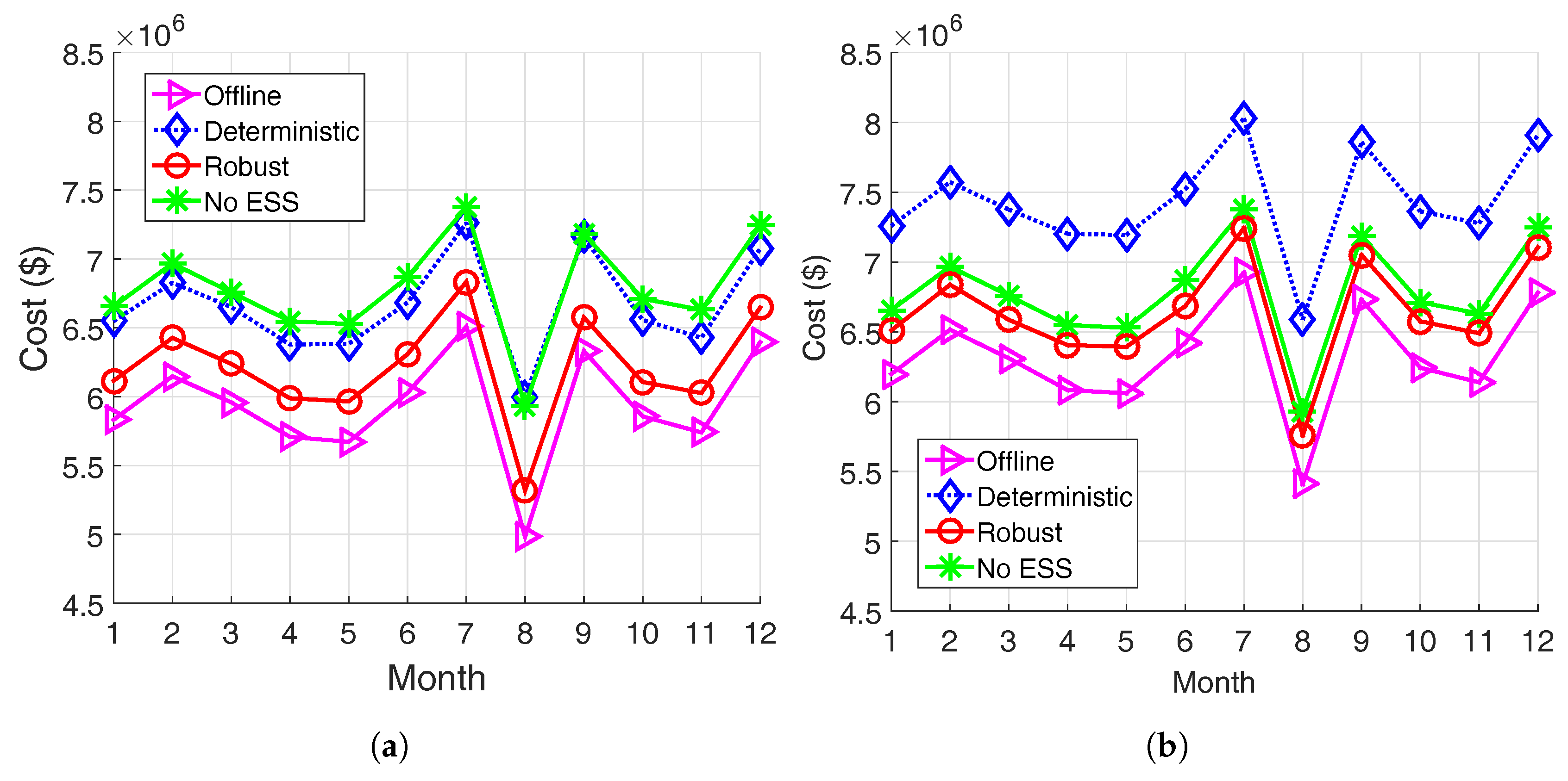
Now we present the results of total cost for year-round operation using the proposed algorithm in Section 2.4. Simulation is performed using two years’ load data. Note that we focus on the second year of operation because it takes one year to be effective due to the memory effect as explained in Section 3.2.
In Figure 10a, we compare the electricity bill without considering battery wear-out cost during operation. As can be seen, electricity bill with robust optimization lies between that of the deterministic case and the offline case. The case of deterministic optimization is almost same to no ESS case, which shows the importance of employing robust optimization. Figure 10b shows the case when battery wear-out cost is computed based on wear density function [18]:
In (25), D denotes the DoD of battery and means the battery cycle life at the level of DoD. a and b are constant variables which determine by battery characteristic. Using these variables, we could apply wear-out density function to define a battery wear-out cost in each time slot,
where denotes the charging/discharging efficiency of battery operation, and s is the SoC level. By differentiating both sides in (26), the wear-out density function is derived as follow,
In ESS optimization process, battery SoC level is calculated in each time slot which makes it possible to calculate total wear-cost by integration of in each time slot. By applying the battery wear-out density function in (27), total cost of the deterministic case becomes even higher than that of no ESS. As a result, robust optimization can save $2,004,200 per year compared with no ESS case.
3.5. Case 4: Battery Capacity and Robust Proportion to Minimize Total Cost
As discussed so far, robust optimization is a proper way to reduce total cost in a real environment. However, to minimize total cost, we should consider the proper battery capacity and robust proportion simultaneously.
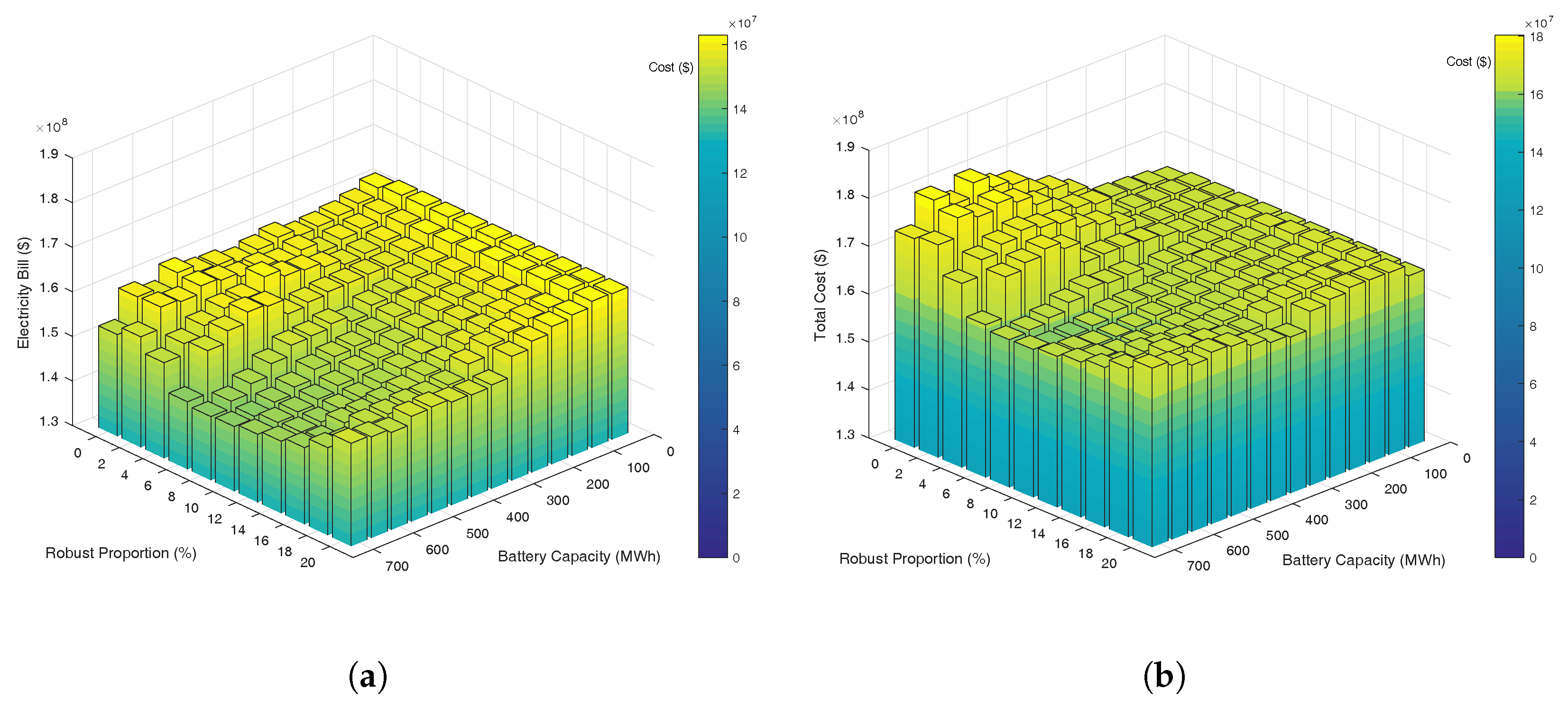
Figure 11 represents the result of electricity bill for different robust proportion and battery capacity considering battery wear-out cost in (27). In Figure 11a, the minimum electricity bill is $144,230,000 when the battery capacity is 700 MWh and robust proportion is 10%. Figure 11b shows the total cost including both electricity bill and battery wear-cost, and the minimum total cost is $165,138,000 when battery capacity is 600 MW and robust proportion is 10%. Note that the desired battery capacity is reduced because battery cost is considered.
We summarize the whole of results using different algorithms in Table 2, which shows the electricity bill, peak load of the year, ESS wear-out cost and the total cost. By using robust optimization, we save $4,585,000 per year compared with the case of no ESS. Furthermore, electricity bill is reduced by $19,840,000 per year. Considering that the ESS installation cost is $150/kWh × 400,000 kWh = $60,000,000, this result implies that return on investment is 3.02 year. The peak load is reduced by more than 3320 kW per year. Since this peak load affects for the next 11 months, the reduced peak load cost is 3320 kW × $8.3/kW × 12 months = $330,672. Since the total peak cost per year is $17,446,932, peak cost is about 10.6% out of the electricity bill case by case. When robust optimization is compared with deterministic case, $19,383,000 is saved.
4. Conclusions
In this paper we propose novel algorithms to minimize the total cost under the Korea commercial and industrial tariff system. In doing this we considered peak load as well as ToU in addition to the regulation of ESS operation. Because the monthly base cost is determined by the 15 min-average peak power consumption and it may affect for 12 months, peak load control should be performed by accurately predicting load profile. However, load prediction errors inevitably exist, and thus we leveraged robust optimization for daily ESS operation. We then extended it to year-round ESS operation based on either active or passive peak load control combined with ToU minimization. By performing Monte Carlo simulations we demonstrated that the proposed algorithm is insensitive to the choice of robust proportion, which makes our algorithm practical. We also considered battery degradation cost using battery wear-out density function. Our extensive simulation with a car manufacturing factory for 24 months confirmed that the proposed algorithm can reduce the peak load by 49.9% and the total cost by 10.8% compared to the case of deterministic optimization. Future work could address when ESS operation is combined with renewable energy, e.g., photovoltaic, which also requires the prediction of renewable generation but generation uncertainty exists.
Acknowledgments
This work was supported by the Korea Institute of Energy Technology Evaluation and Planning (KETEP) and the Ministry of Trade, industry & Energy (MOTIE) of Korea (20161210200360).
Author Contributions
Jangkyum Kim designed the algorithm, performed the simulations, and prepared the manuscript as the first author. Yohwan Choi and Seunghyoung Ryu assisted the project and managed to obtain the load data. Hongseok Kim led the project and research. All authors discussed the simulation results and approved the publication.
Conflicts of Interest
The authors declare no conflict of interest.
References
- Mohsenian-Rad, A.H.; Leon-Garcia, A. Optimal residential load control with price prediction in real-time electricity pricing environments. IEEE Trans. Smart Grid 2010, 1, 120–133. [Google Scholar] [CrossRef]
- Du, P.; Lu, N. Appliance commitment for household load scheduling. IEEE Trans. Smart Grid 2011, 2, 411–419. [Google Scholar] [CrossRef]
- Yan, Y.; Qian, Y.; Sharif, H.; Tipper, D. A survey on smart grid communication infrastructures: Motivations, requirements and challenges. IEEE Commun. Surv. Tutor. 2013, 15, 5–20. [Google Scholar] [CrossRef]
- Sun, S.; Dong, M.; Liang, B. Joint supply, demand, and energy storage management towards microgrid cost minimization. In Proceedings of the 2014 IEEE International Conference on Smart Grid Communications (SmartGridComm), Venice, Italy, 3–6 November 2014; pp. 109–114. [Google Scholar]
- Oudalov, A.; Chartouni, D.; Ohler, C. Optimizing a battery energy storage system for primary frequency control. IEEE Trans. Power Syst. 2007, 22, 1259–1266. [Google Scholar] [CrossRef]
- Isaac Herrera, V.; Gaztanaga, H.; Milo, A.; Saez-de Ibarra, A.; Etxeberria-Otadui, I.; Nieva, T. Optimal energy management and sizing of a battery-supercapacitor-based light rail vehicle with a multiobjective approach. IEEE Trans. Ind. Appl. 2016, 52, 3367–3377. [Google Scholar] [CrossRef]
- Ippolito, M.; Favuzza, S.; Sanseverino, E.; Telaretti, E.; Zizzo, G. Economic feasibility of a customer-side energy storage in the Italian electricity market. In Proceedings of the 2015 IEEE 15th International Conference on Environment and Electrical Engineering (EEEIC), Rome, Italy, 10–13 June 2015; pp. 938–943. [Google Scholar]
- Chaudhari, K.; Ukil, A. TOU pricing based energy management of public EV charging stations using energy storage system. In Proceedings of the 2016 IEEE International Conference on Industrial Technology (ICIT), Taipei, Taiwan, 14–17 March 2016; pp. 460–465. [Google Scholar]
- Erol-Kantarci, M.; Mouftah, H.T. TOU-aware energy management and wireless sensor networks for reducing peak load in smart grids. In Proceedings of the 2010 IEEE 72nd Vehicular Technology Conference Fall (VTC 2010-Fall), Ottawa, ON, Canada, 6–9 September 2010; pp. 1–5. [Google Scholar]
- Nguyen, H.K.; Song, J.B.; Han, Z. Demand side management to reduce peak-to-average ratio using game theory in smart grid. In Proceedings of the 2012 IEEE Conference on Computer Communications Workshops (INFOCOM), Orlando, FL, USA, 25–30 March 2012; pp. 91–96. [Google Scholar]
- Park, D.C.; El-Sharkawi, M.; Marks, R.; Atlas, L.; Damborg, M. Electric load forecasting using an artificial neural network. IEEE Trans. Power Syst. 1991, 6, 442–449. [Google Scholar] [CrossRef]
- Park, S.; Ryu, S.; Choi, Y.; Kim, J.; Kim, H. Data-driven baseline estimation of residential buildings for demand response. Energies 2015, 8, 10239–10259. [Google Scholar] [CrossRef]
- Nguyen, H.K.; Song, J.B.; Han, Z. Distributed demand side management with energy storage in smart grid. IEEE Trans. Parallel Distrib. Syst. 2015, 26, 3346–3357. [Google Scholar] [CrossRef]
- Jeong, M.G.; Moon, S.I.; Hwang, P.I. Indirect load control for energy storage systems using incentive pricing under time-of-use tariff. Energies 2016, 9, 558. [Google Scholar] [CrossRef]
- Taylor, J.W.; McSharry, P.E. Short-term load forecasting methods: An evaluation based on european data. IEEE Trans. Power Syst. 2007, 22, 2213–2219. [Google Scholar] [CrossRef]
- Ryu, S.; Noh, J.; Kim, H. Deep neural network based demand side short term load forecasting. In Proceedings of the 2016 IEEE International Conference on Smart Grid Communications (SmartGridComm), Sydney, Australia, 6–9 November 2016; pp. 308–313. [Google Scholar]
- Ryu, S.; Noh, J.; Kim, H. Deep neural network based demand side short term load forecasting. Energies 2017, 10, 3. [Google Scholar] [CrossRef]
- Han, S.; Han, S.; Aki, H. A practical battery wear model for electric vehicle charging applications. Appl. Energy 2014, 113, 1100–1108. [Google Scholar] [CrossRef]
- Bertsimas, D.; Sim, M. The price of robustness. Oper. Res. 2004, 52, 35–53. [Google Scholar] [CrossRef]
- Soyster, A.L. Technical note convex programming with set-inclusive constraints and applications to inexact linear programming. Oper. Res. 1973, 21, 1154–1157. [Google Scholar] [CrossRef]
- Kim, K.; Choi, Y.; Kim, H. Data-driven battery degradation model leveraging average degradation function fitting. Electron. Lett. 2016, 53, 102–104. [Google Scholar] [CrossRef]
- Choi, Y.; Kim, H. Optimal scheduling of energy storage system for self-sustainable base station operation considering battery wear-out cost. Energies 2016, 9, 462. [Google Scholar] [CrossRef]
Figure 1.
Overall structure of ESS operation.

Figure 2.
An example of predicted load profile of a car factory.

Figure 3.
Analyze the prediction error distribution. (a) Daily error distributions; and (b) seasonal error distributions.
Figure 3.
Analyze the prediction error distribution. (a) Daily error distributions; and (b) seasonal error distributions.

Figure 4.
Result of ESS operation and electric cost in Korea. (a) ESS operation in different algorithms; and (b) time of use pricing in Korea.
Figure 4.
Result of ESS operation and electric cost in Korea. (a) ESS operation in different algorithms; and (b) time of use pricing in Korea.

Figure 5.
Overall structure of year-round operation of ESS.
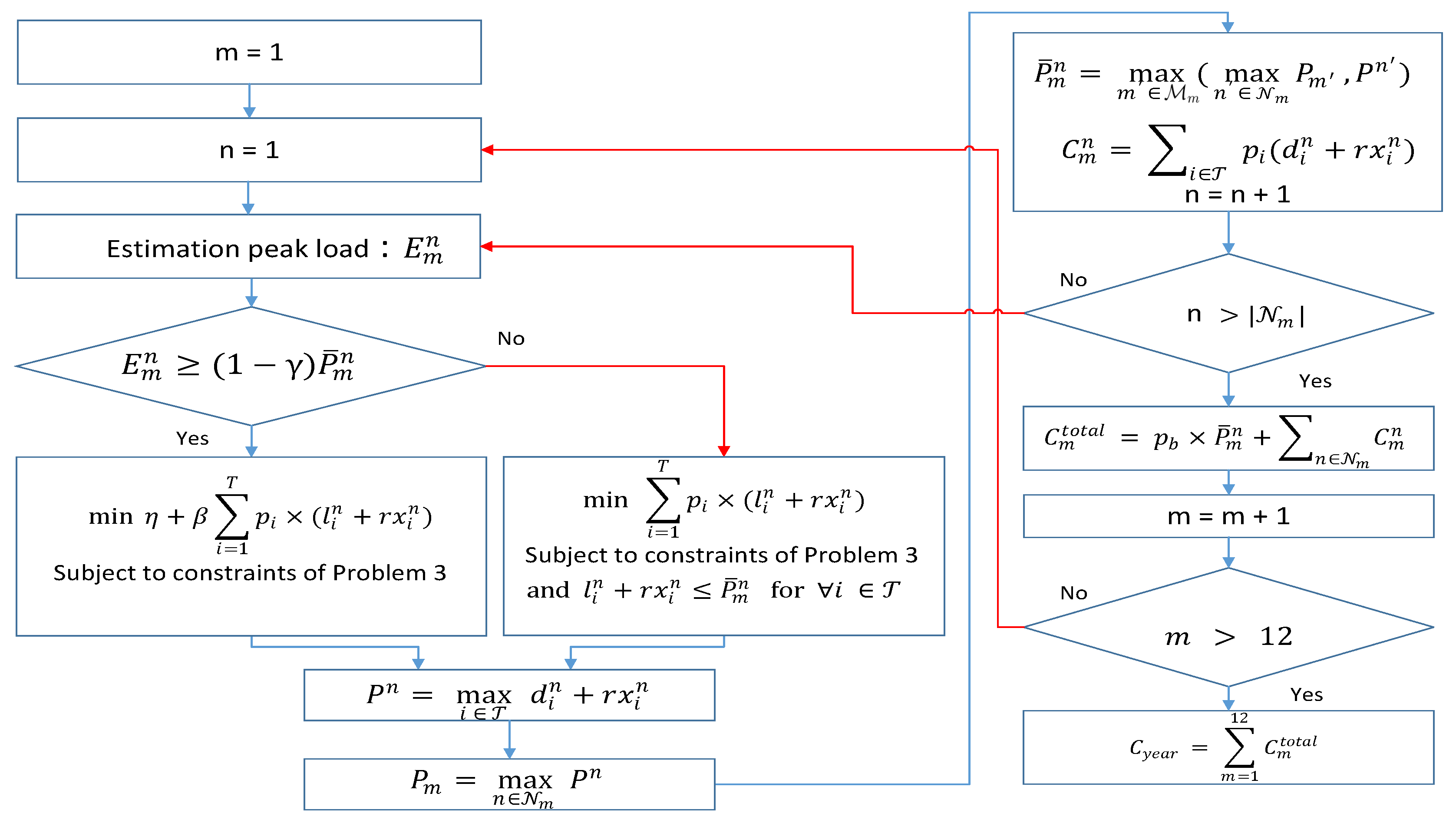
Figure 6.
Real load profile in car factory.
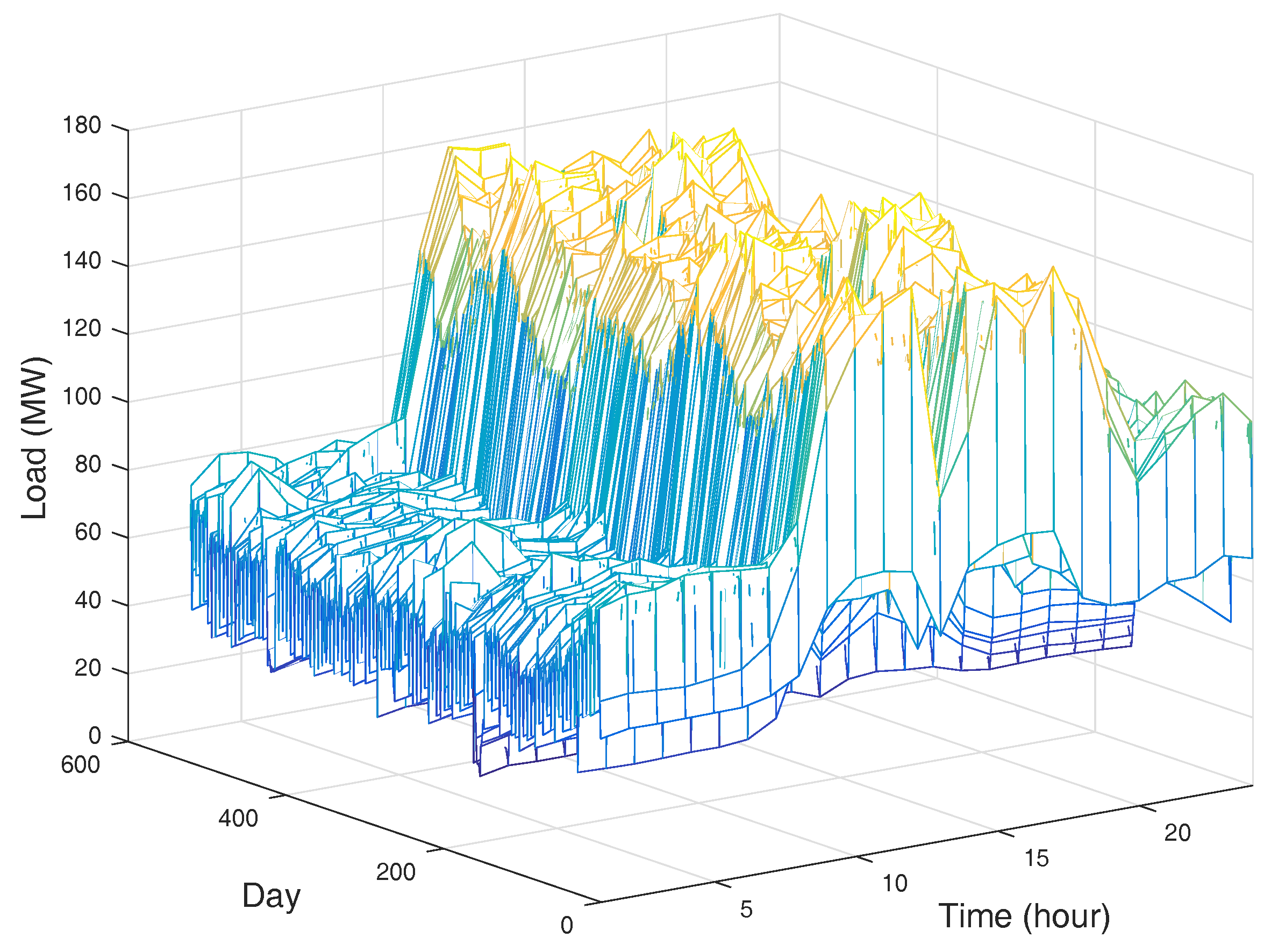
Figure 7.
Peak load control comparison. (a) Monthly peak load; and (b) peak load within one year historical peak load.
Figure 7.
Peak load control comparison. (a) Monthly peak load; and (b) peak load within one year historical peak load.

Figure 8.
Error distribution of load profile.
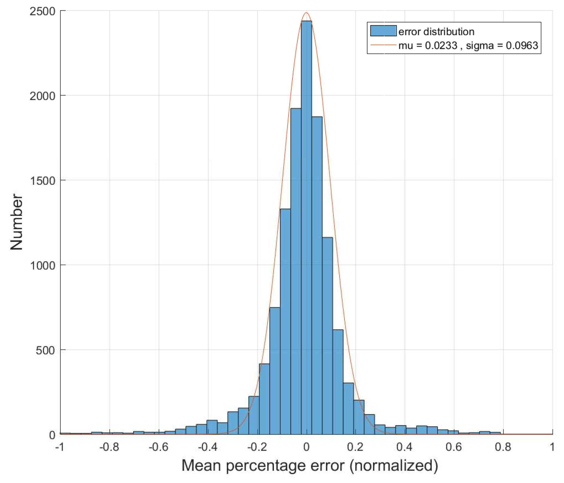
Figure 9.
Result of Monte Carlo simulation. (a) Peak load; and (b) electricity bill in different robust proportion.
Figure 9.
Result of Monte Carlo simulation. (a) Peak load; and (b) electricity bill in different robust proportion.

Figure 10.
Cost comparison in different cases. (a) Electricity bill; and (b) total cost including battery wear-out cost.
Figure 10.
Cost comparison in different cases. (a) Electricity bill; and (b) total cost including battery wear-out cost.

Figure 11.
Cost comparison depending on ESS capacity and robust proportion. (a) Electricity bill; and (b) total cost including battery wear-out cost.
Figure 11.
Cost comparison depending on ESS capacity and robust proportion. (a) Electricity bill; and (b) total cost including battery wear-out cost.

Table 1.
Simulation parameters for case studies.
| Parameters | Symbols | Values (Unit) |
|---|---|---|
| Time interval | − | 15 min |
| Time slot | i | 1–96 (based on 24 h) |
| Battery price | − | $150/kWh |
| Battery type | − | Battery C [22] |
| Battery efficiency | − | 90% |
| Operational SoC range | − | 10%–90% |
| Weighting factor | 1/base electricity price | |
| Initial SOC | 10% | |
| Battery capacity | B | 400 MWh |
| Maximum battery power rate | r | 200 MW |
| Base electricity price | $8.3/kW | |
| Time of Use Pricing | $0.05–0.15/kWh |
Table 2.
Comparison of different algorithms.
| Algorithms | Electricity Bill ($) | Max Peak Load (kW) | ESS Wear-Out Cost ($) | Total Cost ($) |
|---|---|---|---|---|
| Offline | 142,520,000 | 145,530 | 14,490,000 | 157,010,000 |
| Deterministic | 159,760,000 | 342,870 | 19,788,000 | 179,548,000 |
| Robust | 144,910,000 | 171,850 | 15,255,000 | 160,165,000 |
| No ESS | 164,750,000 | 175,170 | 0 | 164,750,000 |
© 2017 by the authors. Licensee MDPI, Basel, Switzerland. This article is an open access article distributed under the terms and conditions of the Creative Commons Attribution (CC BY) license (http://creativecommons.org/licenses/by/4.0/).
Share and Cite
MDPI and ACS Style
Kim, J.; Choi, Y.; Ryu, S.; Kim, H. Robust Operation of Energy Storage System with Uncertain Load Profiles. Energies 2017, 10, 416. https://doi.org/10.3390/en10040416
AMA Style
Kim J, Choi Y, Ryu S, Kim H. Robust Operation of Energy Storage System with Uncertain Load Profiles. Energies. 2017; 10(4):416. https://doi.org/10.3390/en10040416
Chicago/Turabian StyleKim, Jangkyum, Yohwan Choi, Seunghyoung Ryu, and Hongseok Kim. 2017. "Robust Operation of Energy Storage System with Uncertain Load Profiles" Energies 10, no. 4: 416. https://doi.org/10.3390/en10040416
Note that from the first issue of 2016, this journal uses article numbers instead of page numbers. See further details here.