
Research on Control Strategies of an Open-End Winding Permanent Magnet Synchronous Driving Motor (OW-PMSM)-Equipped Dual Inverter with a Switchable Winding Mode for Electric Vehicles

 , ,
, ,
Abstract
:1. Introduction
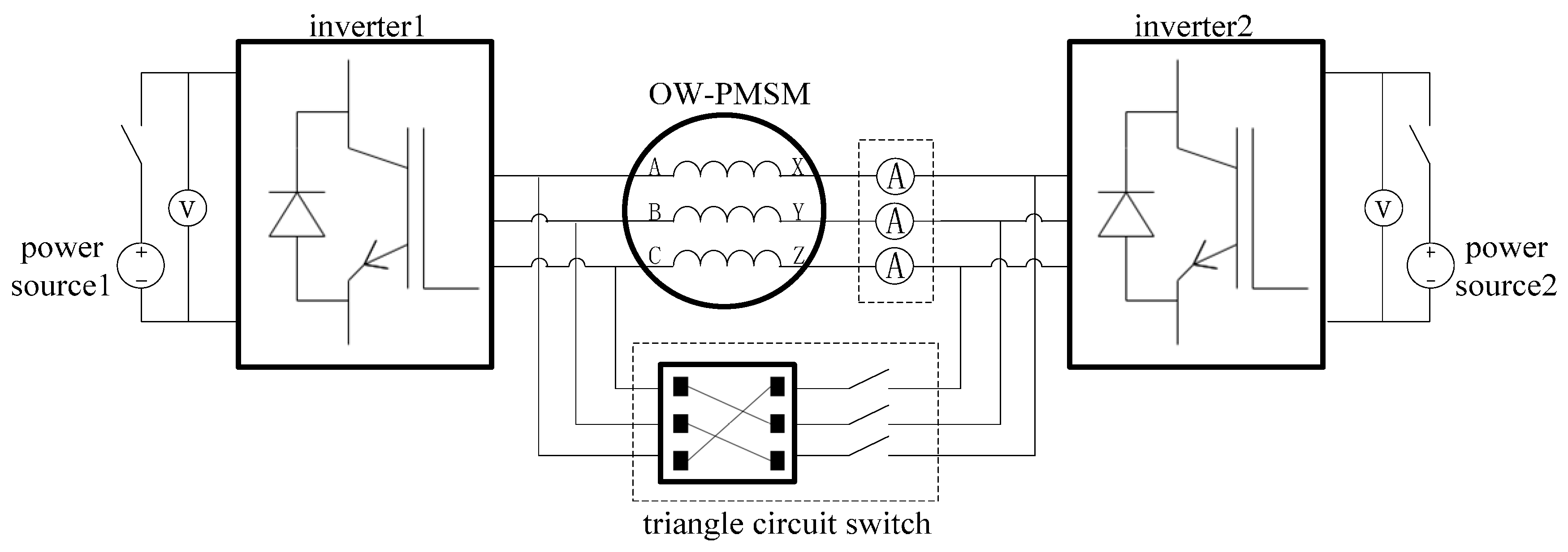
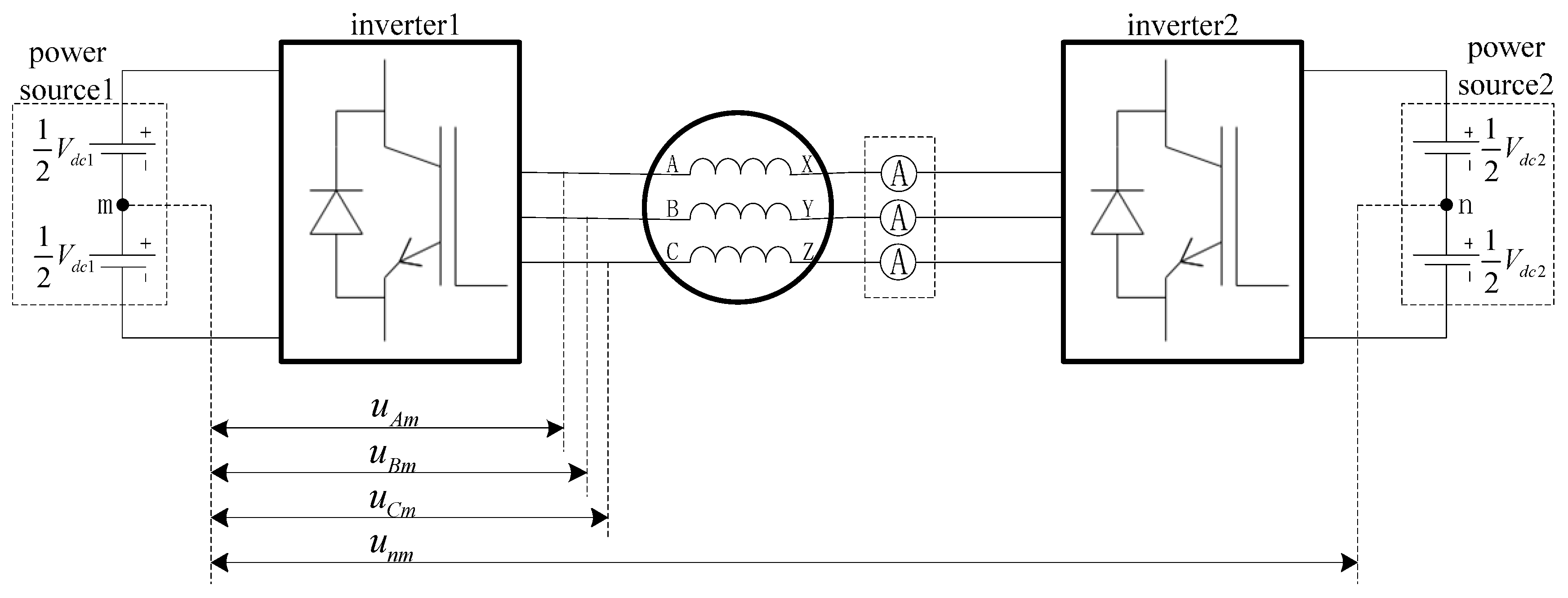
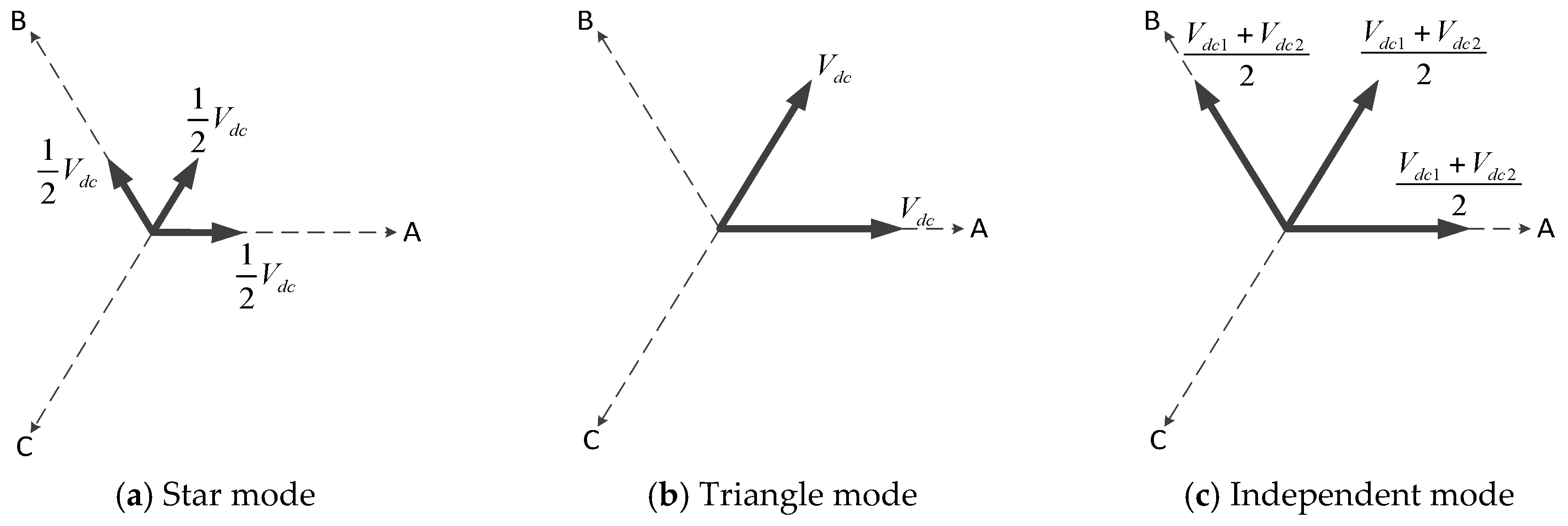
2. Winding Mode Features Analysis and Switching Strategy
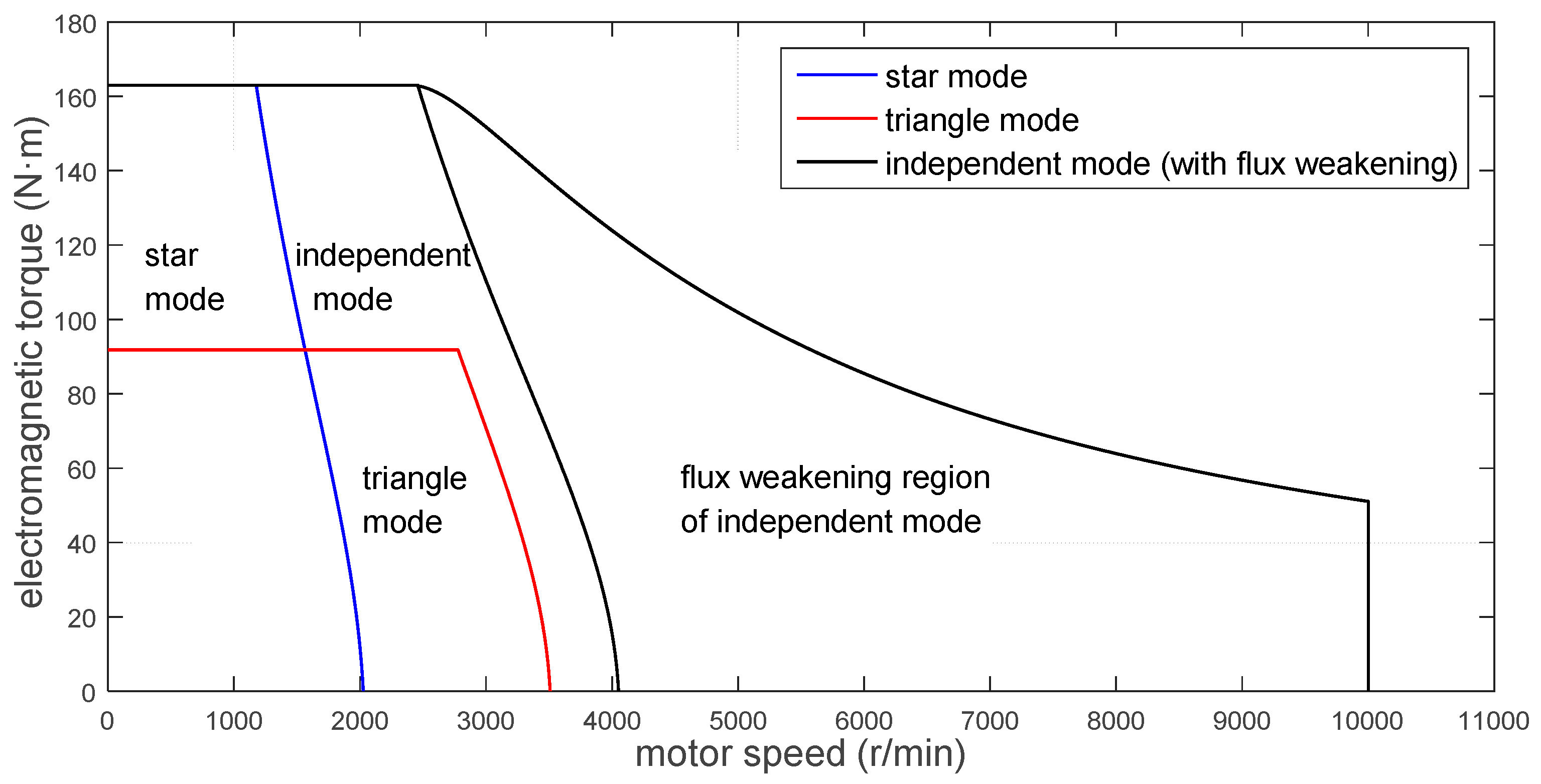
2.1. Winding Mode Features Analysis
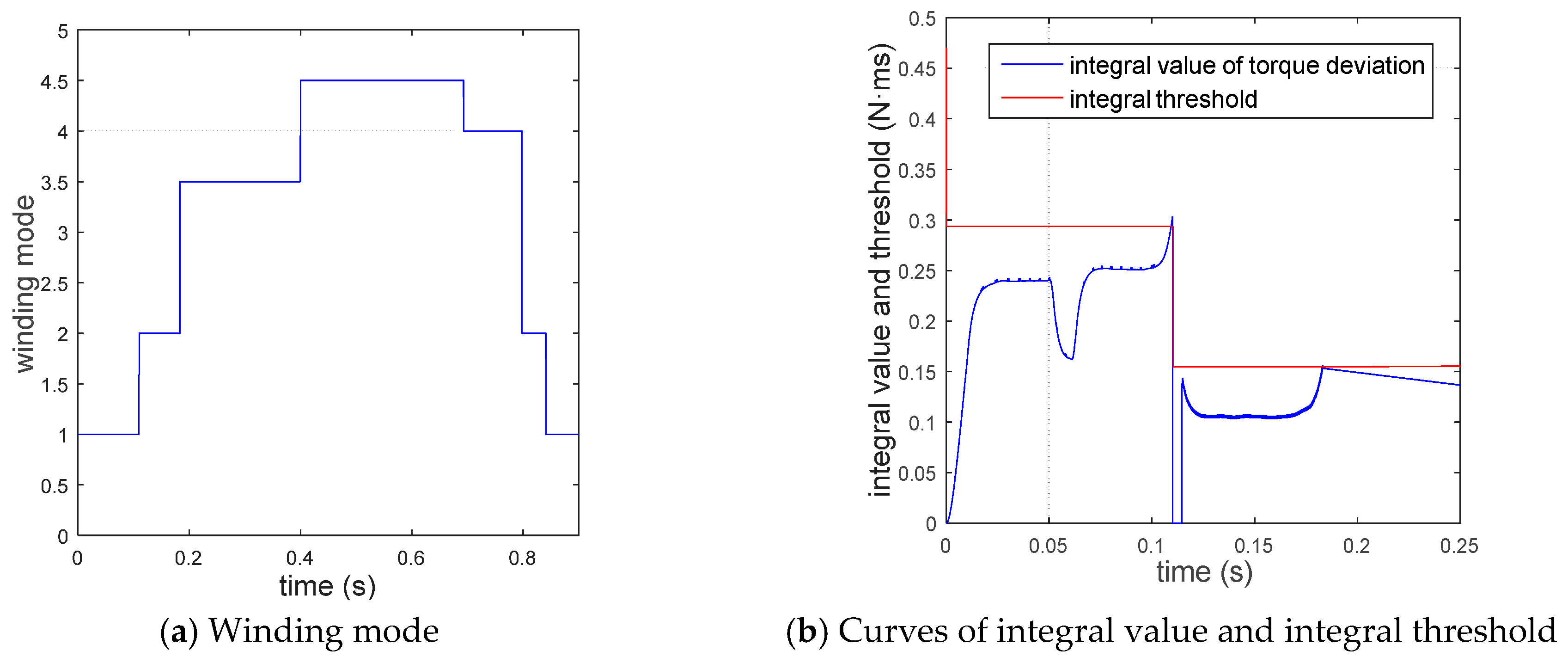
2.2. Winding Modes Switching Strategy
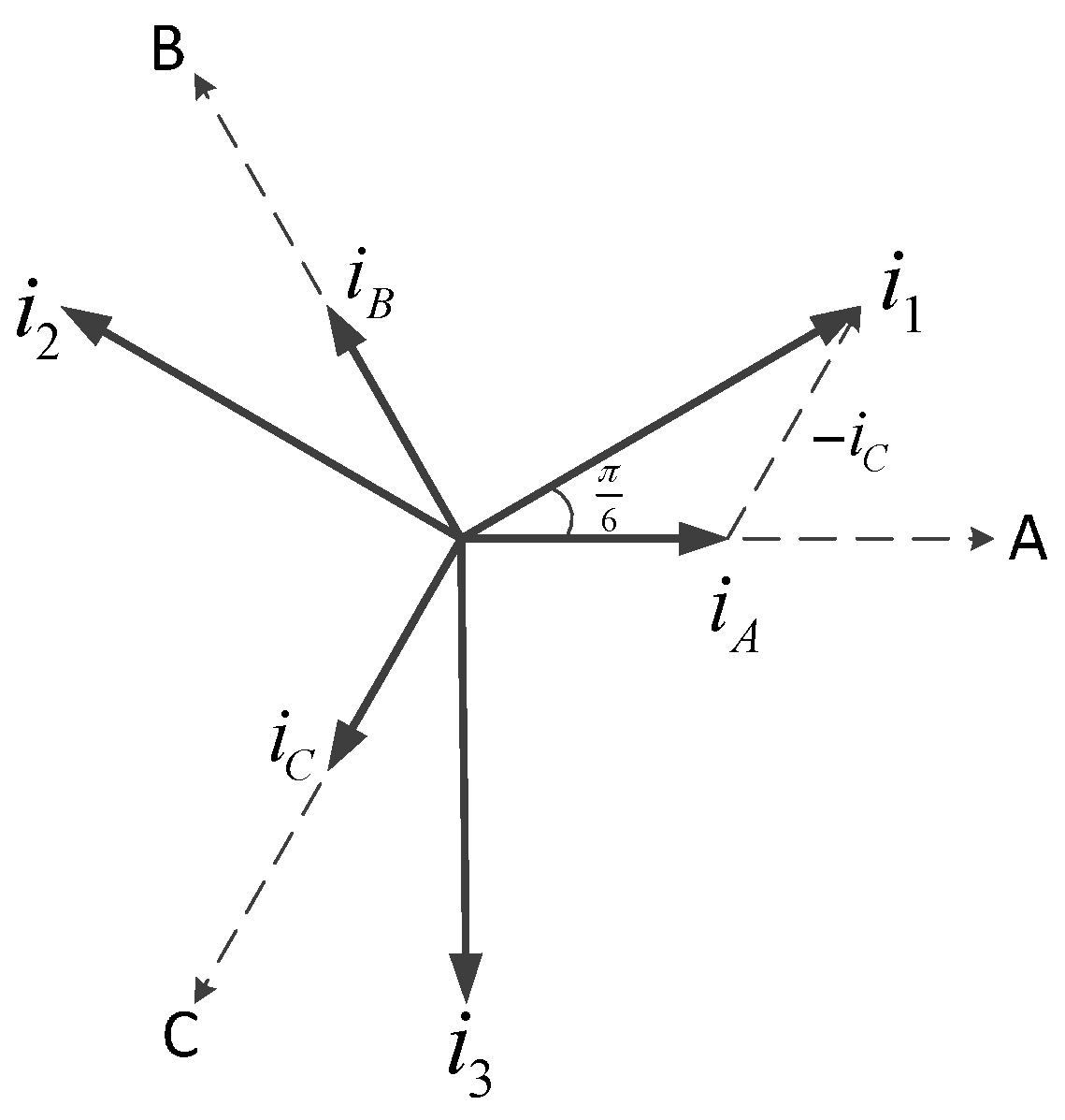
3. Dual Inverters’ Current Modulation Method
3.1. Current Modulation Method in Star and Triangle Modes
3.2. Current Modulation Method in Independent Mode
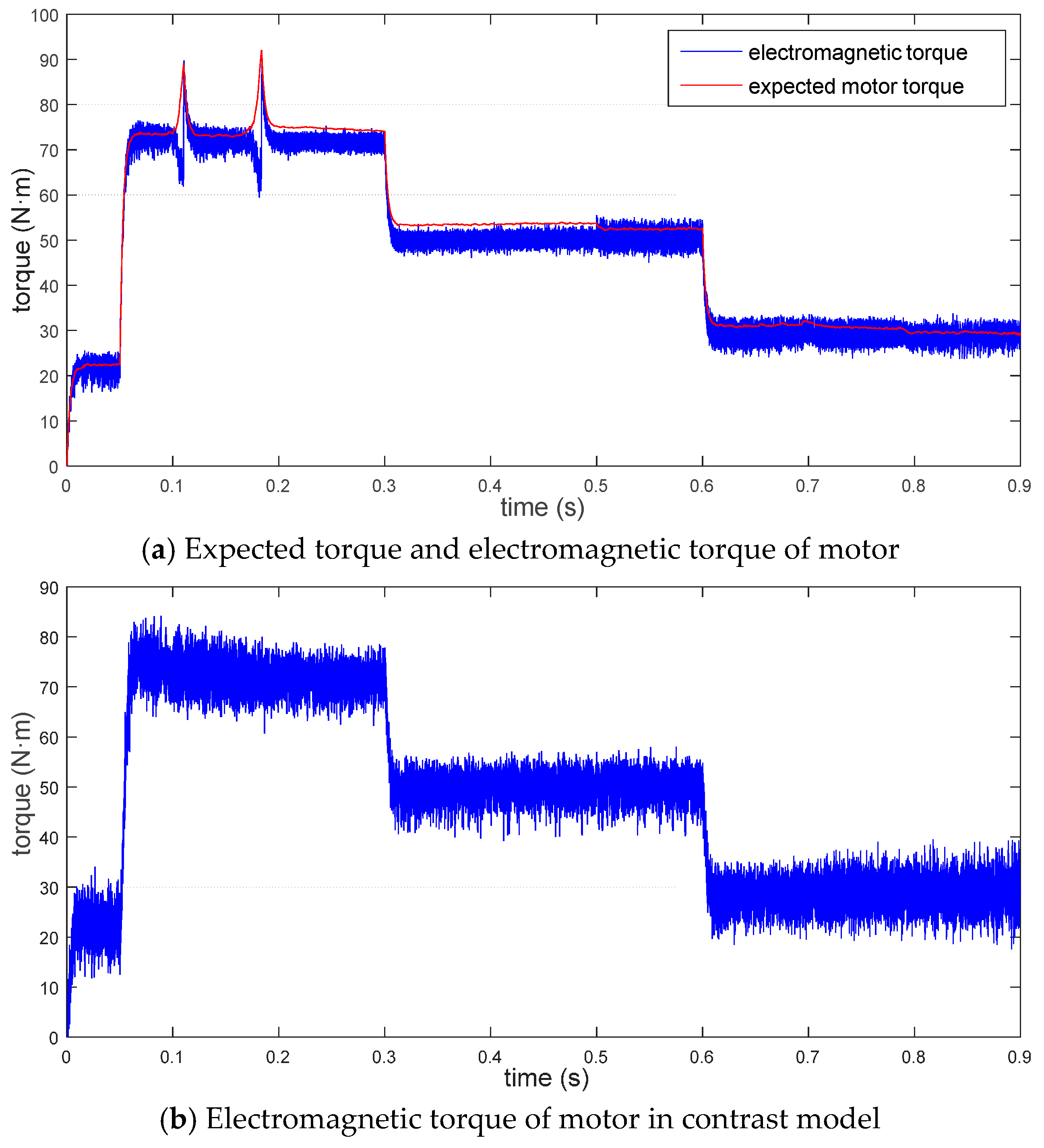
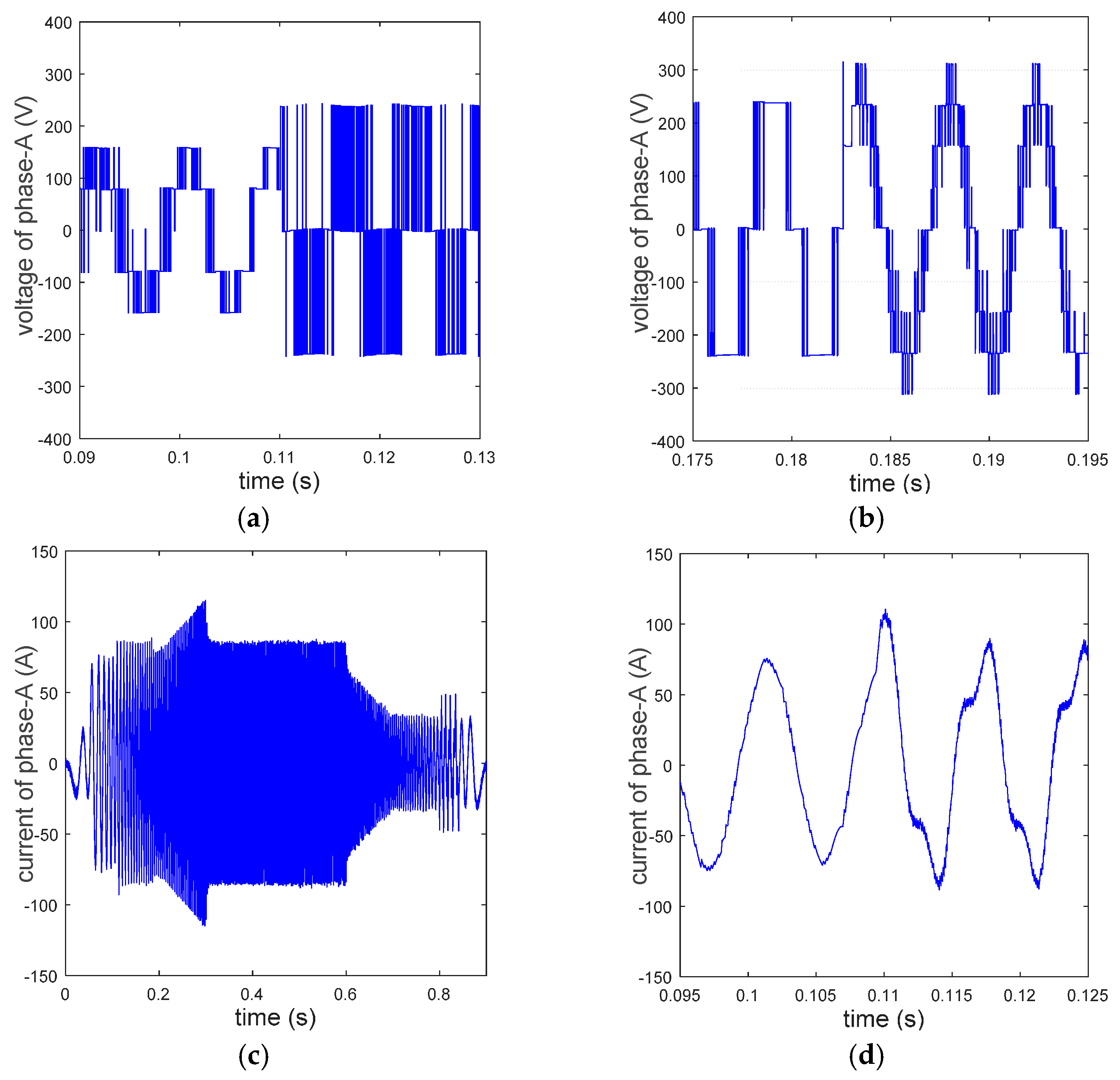
4. Results of Simulations of OW-PMSM Drive System
5. Conclusions
Acknowledgments
Author Contributions
Conflicts of Interest
References
- Chowdhury, S.; Wheeler, P.; Patel, C.; Gerada, C. A multilevel converter with a floating bridge for open-ended winding motor drive applications. IEEE Trans. Ind. Electron. 2016, 63, 5366–5375. [Google Scholar] [CrossRef]
- Loncarski, J.; Leijon, M.; Srndovic, M.; Rossi, C.; Grandi, G. Comparison of output current ripple in single and dual three-phase inverters for electric vehicle motor drives. Energies 2015, 8, 3832–3848. [Google Scholar] [CrossRef]
- Welchko, B.A.; Nagashima, J.M. A comparative evaluation of motor drive topologies for low-voltage, high-power EV/HEV propulsion systems. In Proceedings of the IEEE International Symposium on Industrial Electronics, Rio De Janeiro, Brazil, 9–11 June 2003; pp. 379–384. [Google Scholar]
- An, Q.T.; Duan, M.H.; Sun, L.; Wang, G.L. SVPWM strategy of post-fault reconfigured dual inverter in open-end winding motor drive systems. Electron. Lett. 2014, 50, 1238–1240. [Google Scholar] [CrossRef]
- Engelmann, G.; Kowal, M.; De Doncker, R.W. A highly integrated drive inverter using direct FETs and ceramic dc-link capacitors for open-end winding machines in electric vehicles. In Proceedings of the Applied Power Electronics Conference and Exposition, Charlotte, NC, USA, 15–19 March 2015; pp. 290–296. [Google Scholar]
- Sandulescu, P.; Meinguet, F.; Kestelyn, X.; Semail, E.; Bruyere, E. Control strategies for open-end winding drives operating in the flux-weakening region. Power Electron. IEEE Trans. 2014, 29, 4829–4842. [Google Scholar] [CrossRef]
- An, Q.; Liu, J.; Peng, Z.; Sun, L.; Sun, L. Dual-space vector control of open-end winding permanent magnet synchronous motor drive fed by dual inverter. IEEE Trans. Power Electron. 2016, 31, 8329–8342. [Google Scholar] [CrossRef]
- An, Q.; Sun, L.; Sun, L. Research on novel open-end winding permanent magnet synchronous motor vector control systems. Proc. CSEE 2015, 22, 5891–5898. [Google Scholar]
- Park, J.S.; Nam, K. Dual inverter strategy for high speed operation of HEV permanent magnet synchronous motor. In Proceedings of the Industry Applications Conference 2006, Ias Meeting, Tampa, FL, USA, 8–12 October 2006; pp. 488–494. [Google Scholar]
- Kwak, M.S.; Sul, S.K. Flux weakening control of an open winding machine with isolated dual inverters. In Proceedings of the Industry Applications Conference 2007, Ias Meeting, New Orleans, LA, USA, 23–27 September 2007; pp. 251–255. [Google Scholar]
- Rossi, C.; Grandi, G.; Corbelli, P.; Casadei, D. Generation system for series hybrid powertrain based on the dual two-level inverter. In Proceedings of the European Power Electronic Conferences, Barcelona, Spain, 8–10 September 2009; pp. 1–10. [Google Scholar]
- Griva, G.; Oleschuk, V.; Profumo, F. Hybrid traction drive with symmetrical split-phase motor controlled by synchronized PWM. In Proceedings of the International Symposium on Power Electronics, Electrical Drives, Automation and Motion, Ischia, Italy, 11–13 June 2008; pp. 1033–1037. [Google Scholar]
- Deng, Q.; Wei, J.; Zhou, B.; Han, C.; Chen, C. Research on control strategies of open-winding permanent magnetic generator. In Proceedings of the International Conference on Electrical Machines and Systems, Beijing, China, 20–23 August 2011; pp. 1–6. [Google Scholar]
- Lee, Y.; Ha, J.I. Hybrid modulation of dual inverter for open-end permanent magnet synchronous motor. IEEE Trans. Power Electron. 2015, 30, 3286–3299. [Google Scholar] [CrossRef]
- Casadei, D.; Grandi, G.; Lega, A.; Rossi, C. Multilevel operation and input power balancing for a dual two-level inverter with insulated DC sources. IEEE Trans. Ind. Appl. 2008, 44, 1815–1824. [Google Scholar] [CrossRef]
- Welchko, B.A. A double-ended inverter system for the combined propulsion and energy management functions in hybrid vehicles with energy storage. In Proceedings of the Industrial Electronics Society 2005, IECON 2005, Raleigh, NC, USA, 6–10 November 2005. [Google Scholar]
- Nipp, E. Permanent Magnet Motor Drives With Switched Stator Windings. Ph.D. Thesis, Royal Institute of Techonology, Stockholm, Sweden, May 1999. [Google Scholar]
- Nguyen, N.K.; Semail, E.; Meinguet, F.; Sandulescu, P.; Kestelyn, X.; Aslan, B. Different virtual stator winding configurations of open-end winding five-phase PM machines for wide speed range without flux weakening operation. In Proceedings of the European Conference on Power Electronics and Applications, Lille, France, 2–6 September 2013; pp. 1–8. [Google Scholar]
- Welchko, B.; Nagashima, J.M. The influence of topology selection on the design of EV/HEV propulsion systems. IEEE Power Electron. Lett. 2003, 99, 36–40. [Google Scholar] [CrossRef]
- Nguyen, N.; Meinguet, F.; Semail, E.; Kestelyn, X. Fault-tolerant operation of an open-end winding five-phase PMSM drive with short-circuit inverter fault. IEEE Trans. Ind. Electron. 2014, 63, 595–605. [Google Scholar] [CrossRef]
- Gu, C.; Zhao, W.; Zhang, B. Simplified minimum copper loss remedial control of a five-phase fault-tolerant permanent-magnet vernier machine under short-circuit fault. Energies 2016, 9, 860. [Google Scholar] [CrossRef]
- Zhao, J.; Gao, X.; Li, B.; Liu, X.; Guan, X. Open-phase fault tolerance techniques of five-phase dual-rotor permanent magnet synchronous motor. Energies 2015, 8, 12810–12838. [Google Scholar] [CrossRef]
- Zhan, H.; Zhu, Z.Q.; Odavic, M.; Li, Y.X. A novel zero sequence model based sensorless method for open-winding PMSM with common DC bus. IEEE Trans. Ind. Electron. 2016, 63, 6777–6789. [Google Scholar] [CrossRef]
- Heng, N.; Zeng, H.; Zhou, Y. Zero sequence current suppression strategy for open winding permanent magnet synchronous motor with common DC bus. Trans. China Electrotech. Soc. 2015, 30, 40–48. [Google Scholar]
- Sun, T.; Wang, J.; Chen, X. Maximum torque per ampere (MTPA) control for interior permanent magnet synchronous machine drives based on virtual signal injection. IEEE Trans. Power Electron. 2015, 30, 5036–5045. [Google Scholar] [CrossRef]
- Zhang, Y.; Cao, W.; Mcloone, S.; Morrow, J. Design and flux-weakening control of an interior permanent magnet synchronous motor for electric vehicles. IEEE Trans. Appl. Supercond. 2016, 26, 1–6. [Google Scholar] [CrossRef]


| Items | Parameters |
|---|---|
| Motor type | Interior open-end winding PMSM |
| Number of pole pairs | 4 |
| Stator resistance /Ω | 0.3 |
| Equivalent iron loss resistance /Ω | 90 |
| Fundamental amplitude and third harmonic amplitude of permanent magnet flux linkage [, ]/Wb | [0.2, 0.01] |
| d-axis inductance /F | 0.0012 |
| q-axis inductance /F | 0.0015 |
| Zero sequence inductance /F | 0.0003 |
| Rotational inertia of rotor /kgm−2 | 0.011 |
| Cullen resistance coefficient and viscous resistance coefficient | [0.001, 0.0005] |
| DC bus voltage of power source 1 /V | 240 |
| DC bus voltage of power source 2 /V | 230 |
| Current capacity of inverter device /A | 160 |
| Switching Goal | Star Mode | Triangle Mode | Independent Mode | |
|---|---|---|---|---|
| Starting Mode | ||||
| Star mode | NA | Positive torque saturation decision and | Positive torque saturation decision and | |
| Triangle mode | NA | Positive torque saturation decision | ||
| Independent mode | and | NA | ||
| Direction of Phase Current | |||
|---|---|---|---|
| Inverter Switching States | |||
| Boundary potentials | (01) | Both power sources discharging | Both power sources charging |
| (10) | Both power sources charging | Both power sources discharging | |
| Intermediate potentials | (00) | Power source 1 discharging | Power source 1 charging |
| Power source 2 charging | Power source 2 discharging | ||
| (11) | Power source 1 charging | Power source 1 discharging | |
| Power source 2 discharging | Power source 2 charging |
| Modulation Pattern | Low Switching Frequency Method | High Power Difference Method | |
|---|---|---|---|
| Inverter Switching States | |||
| Boundary potentials | (01) | is in the area of | is in the area of |
| (10) | is in the area of | is in the area of | |
| Intermediate potentials | (00) | crossed control line and switching state of inverter bridge on major power source’s side is 0 | crossed control line and when power source 1 is major power source: phrase current ; when power source 2 is major power source: phrase current |
| (11) | crossed control line and switching state of inverter bridge on major power source’s side is 1 | crossed control line and when power source 1 is major power source: phrase current ; when power source 2 is major power source: phrase current |
| Module Affiliation | Item | Parameters |
|---|---|---|
| Model as a whole | Time step /s | 5 × 10⁻⁷ |
| Inverter devices | On-resistance /Ω | 0.01 |
| Forward voltage drop of IGBT /V | 0.8 | |
| Forward voltage drop of diode /V | 0.8 | |
| Current fall time /s | 1 × 10⁻⁶ | |
| Current tailing time /s | 1.5 × 10⁻⁶ | |
| Winding mode controller | Sampling time /s | 1 × 10⁻⁴ |
| Sensitivity coefficient of rotor speed | [0.9, 0.9] | |
| Sensitivity coefficient of integral threshold | [0.35, 0.75] | |
| PI controller of motor speed | Sampling time /s | 1 × 10⁻⁴ |
| Proportionality coefficient | 0.4 | |
| Integral coefficient | 4 | |
| MTPA and flux weakening controller | Sampling time /s | 1 × 10⁻⁴ |
| Voltage saturation coefficient | 0.95 | |
| Current hysteresis controller | Sampling time /s | 1 × 10⁻⁵ |
| Half width of hysteresis band /A | 3 | |
| Maximum switching frequency of devices /Hz | 1 × 10⁴ |
| Items | Parameters |
|---|---|
| Vehicle weight /kg | 950 |
| Drag coefficient | 0.30 |
| Windward area /m2 | 2.11 |
| Reduction gear ratio | 8.4 |
| Rolling radius /m | 0.307 |
| Rotational mass conversion factor | 1.1 |
| Rolling resistance coefficient | 0.015 |
| Transmission efficiency | 0.95 |
| Rate of braking energy regeneration | 0.6 |
| Driving Cycles | Efficiency Distribution/% | Power Consumption/kWh 100 km−1 | |||||
|---|---|---|---|---|---|---|---|
| ≥0.85 | 0.8–0.85 | 0.7–0.8 | 0.5–0.7 | <0.5 | |||
| Proposed drive system | NEDC | 32.55 | 38.20 | 2.57 | 2.11 | 24.57 | 11.33 |
| UDDS | 44.21 | 14.97 | 9.71 | 7.08 | 24.02 | 10.26 | |
| JC08 | 46.62 | 9.71 | 6.31 | 5.52 | 31.84 | 15.17 | |
| HWFET | 28.41 | 42.52 | 19.33 | 5.36 | 4.38 | 12.52 | |
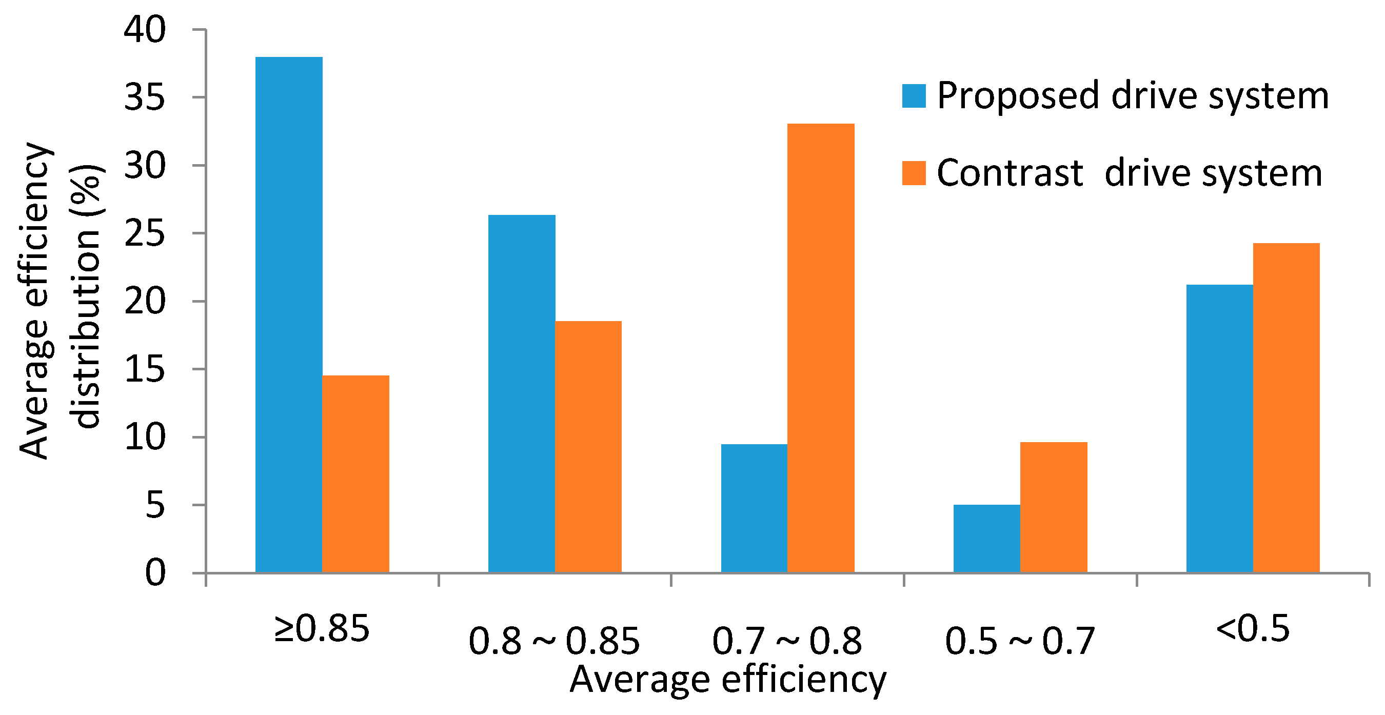
| Average | 37.95 | 26.35 | 9.48 | 5.02 | 21.20 | 12.32 | |
| Contrast drive system | NEDC | 9.79 | 12.92 | 43.18 | 8.15 | 25.96 | 12.18 |
| UDDS | 17.49 | 19.75 | 22.86 | 10.37 | 29.54 | 11.17 | |
| JC08 | 24.66 | 17.14 | 13.74 | 9.55 | 34.91 | 16.23 | |
| HWFET | 6.14 | 24.30 | 52.51 | 10.45 | 6.60 | 13.27 | |
| Average | 14.52 | 18.53 | 33.07 | 9.63 | 24.25 | 13.21 | |
© 2017 by the authors. Licensee MDPI, Basel, Switzerland. This article is an open access article distributed under the terms and conditions of the Creative Commons Attribution (CC BY) license (http://creativecommons.org/licenses/by/4.0/).
Share and Cite
Chu, L.; Jia, Y.-f.; Chen, D.-s.; Xu, N.; Wang, Y.-w.; Tang, X.; Xu, Z. Research on Control Strategies of an Open-End Winding Permanent Magnet Synchronous Driving Motor (OW-PMSM)-Equipped Dual Inverter with a Switchable Winding Mode for Electric Vehicles. Energies 2017, 10, 616. https://doi.org/10.3390/en10050616
Chu L, Jia Y-f, Chen D-s, Xu N, Wang Y-w, Tang X, Xu Z. Research on Control Strategies of an Open-End Winding Permanent Magnet Synchronous Driving Motor (OW-PMSM)-Equipped Dual Inverter with a Switchable Winding Mode for Electric Vehicles. Energies. 2017; 10(5):616. https://doi.org/10.3390/en10050616
Chicago/Turabian StyleChu, Liang, Yi-fan Jia, Dong-sheng Chen, Nan Xu, Yan-wei Wang, Xin Tang, and Zhe Xu. 2017. "Research on Control Strategies of an Open-End Winding Permanent Magnet Synchronous Driving Motor (OW-PMSM)-Equipped Dual Inverter with a Switchable Winding Mode for Electric Vehicles" Energies 10, no. 5: 616. https://doi.org/10.3390/en10050616