
Multi-Objective Dynamic Economic Dispatch with Demand Side Management of Residential Loads and Electric Vehicles


1
Department of electrical and computer engineering, Missouri University of Science and Technology, Rolla, MO 65401, USA
2
Lawrence Berkeley National Laboratory, Berkeley, CA 94720, USA
*
Author to whom correspondence should be addressed.
Energies 2017, 10(5), 624; https://doi.org/10.3390/en10050624
Submission received: 22 January 2017
/
Revised: 26 April 2017
/
Accepted: 27 April 2017
/
Published: 3 May 2017
(This article belongs to the Section F: Electrical Engineering)
Abstract
:In this paper, a multi-objective optimization method based on the normal boundary intersection is proposed to solve the dynamic economic dispatch with demand side management of individual residential loads and electric vehicles. The proposed approach specifically addresses consumer comfort through acceptable appliance deferral times and electric vehicle charging requirements. The multi-objectives of minimizing generation costs, emissions, and energy loss in the system are balanced in a Pareto front approach in which a fuzzy decision making method has been implemented to find the best compromise solution based on desired system operating conditions. The normal boundary intersection method is described and validated.
1. Introduction
Demand side management is an approach through which consumer demand can be shaped to improve power system generation and load balance [1,2]. In addition, demand side management (DSM) programs may be implemented to improve load factors or to defer capital investment in system expansion. In the United States, demand response programs during 2011 generated approximately $6 billion in direct revenues for local businesses, industry, and households through investment costs avoidance [3]. For example, the Pennsylvania-Jersy-Maryland (PJM) seasonal peak was reduced by 7% through the implementation of regional DSM [3].
The majority of current DSM applications target large industrial consumers due to ease of coordination coupled with a large return on investment [4]. However, advances in communication technologies as well as load control at end-use points are expected to encourage further implementation of demand side management among smaller customers in residential and commercial sectors [5,6]. Home energy management systems will provide improved capabilities to coordinate load demand with market incentives through appliance load and Plug-in electric vehicle (EV) charging deferral and aggregation.
EV may become a significant portion of the future distribution load, and may also play a large role in DSM programs due to their flexibility in charging schedules. The penetration of EVs is expected to increase drastically in the next few years, which can reach one million by 2015 in US [7]. It is because of their undeniable benefits such as reducing the emission level [8,9]. However, increasing the penetration level of EVs can burden the grid and, in the absence of a proper charging control strategies, it can easily overload the electricity grid at peak hours. In addition, uncoordinated charging of electric vehicles by the customers can impose problems on the distribution network like increasing the peak demand, voltage sags, congestion, thereby leading to increased losses, reduced component lives and bringing up of costly generators to serve the excess load. This might eventually result in a need for infrastructural reinforcements, increase in the price of electricity and power quality problems.
A good solution for preventing problems imposed by the EVs on the grid is to devise effective coordination techniques to optimally charge the vehicles on one hand and incentivize the customers to get enrolled in such programs on the other. An optimal charging strategy is one that charges the vehicle within the time available as per the customer’s convenience while considering the network loading e.g., reducing the peak-time connections and filling the valley in the load profile during night. This study proposed a charging model for EVs, which is explained in detail in the following section.
All of the above positive effects of DSM and EV coordination charging depend on customer participation in the load shifting programs. Financial incentives are not wholly sufficient to guarantee consumer participation in DSM programs; consumer comfort must not be significantly degraded, which requires assurances of appliance and vehicle availability. Therefore, the load shaping aspect of DSM requires an optimization that incorporates multiple, and possibly competing, constraints. In addition to load management, the utility provider may also desire to reduce operating costs and/or other functionalities such as carbon emissions or energy loss. Therefore, to fully exploit the load shaping capabilities of DSM programs, the DSM must be simultaneously coupled with an economic dispatch approach such that the overall system is optimized. Thus, a unified optimization must provide simultaneous schedules for both the generation and load, requiring a unified multi-objective approach to balance competing schemes for different considered objectives—here, generation cost, emission, and energy loss.
Over the past few years, rising concern over the environmental issues and the passage of the US Clean Air Act amendments of 1990 has forced the utilities to modify their operation strategies for generating the electric power at a lower pollution. In the past, some techniques have been presented to reduce the emission in power plant such as utilization of low-emission fuels, alternate energy resources, and emissions dispatching. In addition, flattening the load profile using demand response programs can preclude bringing up of high polluted generators to serve the excess load [10]. The first two solutions require modification of the existing power plant or installation of some equipment, which require a large investment. Furthermore, the necessity of emission dispatching is changing the most economic generation schemes from an economic dispatch point of view. Therefore, the last solution can be more appropriate for reducing emissions compared with other techniques.
Another important issue in power system operation is the loss reduction, in which the system operator tries their best to minimize it as much as possible. In the process of transmitting the generated power, an estimated four percent of the total energy produced is lost. The economic viability of power systems, especially in a competitive energy market, demands an optimum mix of all of the parameters that influence power generation and transmission. An approach to achieving this optimum is to include the transmission losses as one of the objectives in the economic dispatch (ED) problem [11]. To this, DSM is employed to reduce energy loss, besides generation cost and emission in this approach. Our proposed model aims to minimize the total electricity cost, loss, and emissions while considering user comfort, EV travel patterns, and EV electricity demand. Therefore, it is necessary to combine the demand side management and dynamic economic dispatch (DED) to take the generation and the demand into account.
Tons of studies have been dedicated to the dynamic economic dispatch problem and the effect of deferrable loads on power system operation during the past few years. Shao et al. presented a load shaping tool based on DR strategy to reduce the impact of EV on the distribution grid. They take customer preferences, comfort level and load priority into account [12]. Their method is able to manage the total demand, preventing the transformer from being overloaded. However, the studied system is limited to a residential transformer serving three homes. In addition, EV contribution is included through a simple policy with no modeling of EV load management.
Abdi et al. proposed dynamic economic dispatch problem integrated with demand response. They derived economic models of the linear and nonlinear responsive loads for time-based and incentive-based demand response programs and integrated them with DED. However, the customer comfort and EV coordination is not considered in their approach [13]. Papavasiliou and Oren proposed the unit commitment model for assessing the reserve requirements resulting from the large-scale integration of renewable energy sources and deferrable demand in power systems. They presented a demand response paradigm for assessing the benefits of shifting deferrable loads [14]. Muratori et al. reviewed market-related problems of modern electric grids and possible solutions to address them. Specifically, they proposed a techno-economical solution, namely, residential demand response programs enabled by a smart grid [15].
In our previous works [16,17], the effect of demand side management of appliances on the reliability, loss, and voltage profile of power systems are studied. Even though the customer comfort is taken into consideration, the economic aspects of the DSM are not evaluated. The impact of EVs on the demand profile is analyzed in [18,19], and the authors try to consider EV and demand response strategies. In both studies, EV contribution is considered through simple policies without mathematical modeling for EV coordination. In [20], a game theoretic approach is proposed to schedule EV charging for load profile management. Vehicle-to-grid (V2G) capability has been considered in [21], for developing an optimization problem in order to manage the load profile. Oviedo et al. [22] proposed a coordination mechanism to allocate EV charging efficiently. An optimization-based model is presented in [23] to perform load shifting in the smart grid environment. In this model, different agents for load, generation and storage management are defined and V2G is considered.
Efficient EV charging strategies are derived using EV traveling pattern in [24,25]. Rotering et al. proposed a dynamic programming based optimization method for one EV using available electricity prices and EV driving patterns [26]. Wu et al. considered load scheduling and dispatch problem for a fleet of EVs in both the day-ahead market and real-time energy market [27]. Nguyen and Le presented the joint optimization of electric vehicle (EV) and home energy scheduling in order to minimize the total electricity cost while considering user comfort preferences [28]. Paterakis et al. presented a home energy management system for determining the optimal day-ahead appliance scheduling under hourly pricing and peak power limit based strategies [29].
Muratori and Rizzoni presented a dynamic energy management framework to simulate automated residential demand response. The optimal schedule of all the controllable appliances, including electric vehicles, is found by minimizing consumer electricity-related expenditures [30]. Mahmoodi et al. introduced a distributed economic dispatch strategy for microgrids with multiple energy storage systems. Their strategy overcomes the challenges of dynamic couplings among all decision variables and stochastic variables in a centralized dispatching formulation [31]. Shamsi et al. proposed an agent based community microgrid for solving the dynamic economic dispatch (ED) problem in which each agent is capable of trading electricity with other agents through a local energy market [32]. However, they didn’t take the DSM and EV effects into account.
The appliance scheduling and electric vehicle charging problems are often addressed separately in the literature, and, to the best of our knowledge, none of the previous works have considered a multi-objective based approach for detailed design and joint optimization of EV and building energy management. To this end, we propose a unified optimization model that jointly optimizes the scheduling of EVs and household appliances while different constraints including generator limits, load balance, and load shifting are observed. There are several techniques mentioned in articles to solve multi-objective problems such as reducing the multi-objective problem into a single objective one by treating other objectives as a constraint, or uniting all the objectives into a single objective function. There are some drawbacks associated with these methods, such as the limitation of the available choices and their prior selection need of weights or targets for each of the objective functions. In addition, the weighted sum method is often preferred to form the tradeoff surface. However, two major disadvantages exist: if the Pareto set is non-convex, the Pareto points on the concave parts of the trade-off surface will be missed and, for an even spread of the weights, the optimal solutions in the criterion space are not usually evenly distributed. To this end, a Pareto-based approach that can obtain a set of optimal solutions instead one is employed. In addition, this paper takes advantage of a fuzzy decision method to find the best Pareto optimal solution among all of the Pareto solutions based on the operator desire. Power system operators can select one of these solutions in accordance with their previous experience.
The proposed study focuses on the load rescheduling where there is no net reduction in the load, but it is rescheduled to different times over the time horizon. In general, if the consumption profile of a load is going to be manipulated, there must be some slack in its energy consumption. Slack is a measure of the potential of an energy load to be advanced or deferred without affecting earlier or later operations or outcomes. With this in mind loads, it can be divided into on demand, deferrable, and flexible loads categories. On demand loads are often directly connected with consumer action and must be supplied when requested, such as turning on lights, providing zero slack in operation. Deferrable loads may permit scheduling of the energy consuming action, with little physical consideration or cost associated with deferring or initiating the action; these are often atomic actions that once started run to completion, like a washing machine load. Flexible loads permit some elasticity in consumption, within certain constraints often associated with the physics of the process; charging a battery is an example [33]. For brevity, only deferrable loads are considered in this study. Furthermore, postponing the process or load activities is easy because the load is discarded at a critical time so the process has to catch up later. To this purpose, just the postponing process has been considered for deferrable loads.
Some DSM methods proposed in literature affected the overall system demand only and did not use detailed load models in the network [29], which can disturb the customer comfort. As a matter of fact, the success of a demand response program is directly tied to occupants’ perceived comfort and satisfaction. To this end, the proposed approach explicitly models these constraints in the optimization process by the consumers’ acceptable delay times (ADTs) and the penetration level of active consumers, which is the portion of responsive customers to total customers. An ADT presents the maximum period of time by which the operation of the associated appliance can be prolonged without disrupting the customers’ comfort. It is notable that the ADT for nondeferable loads is zero, since customers’ comfort will be sacrificed by any delay in their operation. Information on the ADT value for different appliances can be derived by exploring consumers’ preferences from questionnaires and survey data. In addition, the penetration level of active customers is defined as the average customers’ willingness to respond. Indeed, penetration level is the ratio of the number of active customers to the total number of consumers [34]. An active customer is one who simply changes consumption of its responsive appliances upon receiving a signal from the load aggregator [35]. It is worth noting that there are different ways to shift the loads such as rescheduling business operations to off-peak hours or at night, or immediate interruptions on operating machines in business premises for approximately one to two hours. Therefore, both forward and backward load shifting can be implemented to shave the loads. However, postponing the process or load activities is easy because the load is discarded at a critical time so the process has to catch up later. However, the quality of the process may not be consistent. Toward this end, only the postponing load shifting process is considered in this study.
In order to implement the proposed approach, every house should receive relevant input information from Load Serving Entities (LSE) and plans the operation of all electrical equipments [35], which can be easily done by the recent technology. The proposed energy management framework introduced in this paper is centralized in the sense that all households receive a signal from the electric utility and simultaneously optimize their demand. We believe that a centralized solution is the preferred approach under current technological capabilities. Furthermore, since the control signal is sent by the aggregator, adaptation will be easier. Lastly, it can be contended that consumer confidence can be won through pricing incentives. Thus, in this study, a centralized scheduling approach has been presented.
The contribution of the proposed study is introducing a centralized multi-objective model for implementing the demand side management, without sacrificing customers’ comfort, to optimize the generation cost, loss, and emission in power system. Furthermore, the proposed approach is simple in concept and easy to implement. In addition, it can be expanded easily to implement in a larger case study with more generators and households.
2. Modeling
The basic approach in the unified optimization model is to minimize the costs of generation, emissions, and energy loss subject to the DSM load shaping constraints.
2.1. Generation
The optimal solution is a constrained minimization. The cost of generation, emissions, and transmission losses may all be modeled as a function of the individual (ith) generator outputs . The costs are then minimized over the time intervals of interest for The individual time increments may be arbitrarily selected, but are typically taken as an hour, or a fraction thereof. The proposed problem includes minimization of three objective functions expressed as follows:
- (1)
- Generation cost
- (2)
- Emission
- (3)
- Energy loss
subject to
while simultaneously shaping the system load through DSM to achieve this minimum. This requires determining a schedule in which home appliances may be deferred up to their acceptable delay times (to ensure consumer comfort) and an acceptable EV charging schedule in which all vehicles are fully charged by the time the consumer commuter leaves home. The total generation cost is given in Equation (1), where , , are the cost function coefficients of the ith unit, respectively. is the active power generation of the ith generator at the tth time interval. Equation (2) determines the total emissions, where , , and are the emission cost coefficients of the ith unit. The emissions objective function can incorporate multiple types of generator output with suitable parameters. Equation (3) is the energy loss in the system over the time interval of interest. The active power losses at time t, , are modeled by the quadratic loss formula:
where , , and are the loss coefficients such that is a matrix, is an vector, and is a scalar constant. The generator outputs are subject to inequality constraints describing the physical output limits of the generators:
where and are the maximum and minimum active power output limits of the ith generator. Furthermore, the change in generator output of all online units is restricted by its ramp rate during each dispatch period:
where and are the power outputs (in MW) of unit i at the tth and st time intervals. and are the up and down ramp-rate limits of each unit in MW/hour.
2.2. Deferrable Appliances
The approach used in this paper is generalized from several previous studies. The approach proposed in this paper merges and extends the results of [29,30] to develop a comprehensive flexible load model. The deferrable appliance load model is predicated on the assumption that the energy requirement of the load may be shifted to a different time period within the acceptable time horizon. The load energy requirement is not reduced by deferral; it is merely delayed. The load flexibility is modeled by consumers’ acceptable delay times (ADTs) and the penetration level of active consumers. A household load typically consists of both deferrable and nondeferrable loads. A participating, or active customer, is one whose responsive appliances modify their consumption based on a command from the load aggregator, or Load Serving Entity (LSE) [35]. Four types of appliances including dishwashers, clothes washers, clothes dryers, and heating and ventilation systems are considered as responsive loads. Their ADT values are provided in Table 1. An ADT of 2 h for the heating and ventilation load implies that this load may be deferred up to 2 h without adversely impacting consumer comfort. The load is considered to be non-elastic, which implies that the energy requirement does not increase nor decrease by being delayed. Characterization of the ADT values for different appliances can be obtained from consumer questionnaires, survey data, or program enrollment conditions [34]. The ADT values can be varied for different users and considering the same ADT for all customers can be a kind of oversimplification. However, the proposed approach is easily expandable to consider multiple customers with different ADTs.
The constraint equations describing the system load is:
where at time t is composed of : non-deferrable load, : normally scheduled deferrable load, : load that has been shifted into or out of interval t. Note that, by this definition, may be positive or negative. The (constant) is the sum of the individual appliance loads in the set A of all deferrable appliances normally scheduled at time t:
where “normally scheduled load” refers to the load that would occur during a given time interval if no load shifting occurred. The shifted load is the sum of all loads shifted into time t from previous times less the sum of flexible loads shifted to future times
where is the load of appliance a that is shifted from to and is the acceptable delay time of appliance a. The first summation on the right-hand side of Equation (11) represents the normally scheduled load that has been shifted from previous time intervals to the current time interval, whereas the second summation represents the normally scheduled load that has been shifted from the current time interval to future time intervals. Furthermore, load may only be delayed and may not be shifted to an earlier time interval. Therefore,
Lastly, to ensure the shifted load cannot exceed the normally scheduled deferrable load:
2.3. Electric Vehicle Loads
Electric vehicles (EVs) are becoming increasingly more prevalent due to their environmental benefits and costs. However, the increased penetration level of EVs can burden the grid and can easily overload the electricity grid during peak hours if not properly coordinated. Uncoordinated charging of electric vehicles can result in problems in the distribution network such as increased peak demand, decreased component life, voltage sags, and congestion. One solution for preventing the problems imposed by the EVs on the grid is to develop individual charging strategies to minimize their cumulative impact. To accomplish this goal, EVs can be coupled with demand response by treating the EVs as deferrable loads. However, since EV energy requirements are typically much higher and longer than household appliances, special considerations are required for their inclusion in DSM. The impacts of EVs on the demand profile have been initially addressed in [18,19], in which the EVs are incorporated into the demand response strategies. In these studies, the EV contribution is deployed through simple heuristic policies without explicit mathematical modeling of the EV load management. Similarly, in [20], a game theoretic approach is proposed to schedule EV charging for load profile management and [22] proposes a coordination mechanism to allocate EV charging efficiently. Using these preliminary studies as a starting point, the EV and demand response approaches will be extended and generalized for a more comprehensive approach to load profile optimization. To incorporate the EVs into the optimization Equations (1)–(13), they must first be modeled in an appropriate manner for inclusion in the mathematical framework. The first step is to use an aggregation technique to group vehicles with similar energy requirements together. This aggregation assists in permitting each group to be treated like an appliance with an acceptable delay time. For example, if a vehicle requires 4 h of charging, it has an ADT of 8 h in a 12 h charging window. All vehicles with the same charging requirements impose similar loads on the system. This is analogous to an appliance with certain energy requirement every hour and a user-defined ADT. It is noteworthy that the stochastic EV scheduling has not been considered in this study, as the proposed problem itself has been designed as a deterministic day-ahead problem. However, considering the stochastic nature of the EVs is a desirable avenue of research that authors have in mind for the future work. Interested readers are directed to [36,37] for more information about the stochastic modeling of EVs. To model the vehicle load, the following assumptions are made:
- The charging window is fixed between hour 8:00 p.m. and hour 8:00 a.m. Because the majority of vehicles are available for residential charging at this time, we assume that there are 12 possible connection times within the charging time frame (on the hour), but this can be expanded to any number of possible connection times without loss of generality (e.g., every 15 min), with added computational complexity [38],
- all information on the driving profiles is available,
- the vehicles are charged at home with a Type-1 charger with a maximum rating of 1.44 kW,
- the number of EV households is the same as those participating in the appliance deferral DSM program.
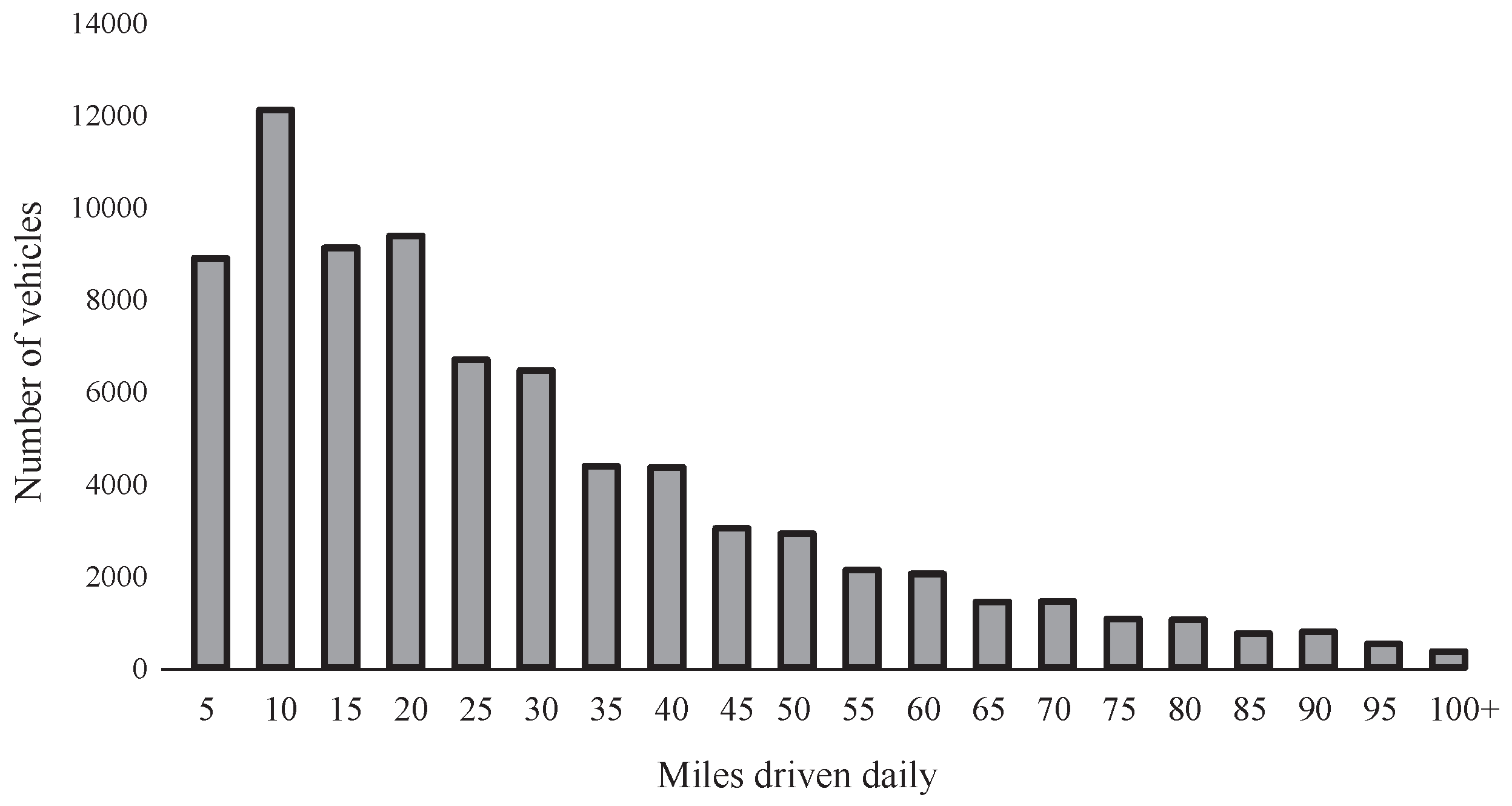
Based on data taken from the 2009 National Household Travel Survey, the EVs have been aggregated into 20 groups based on their daily commute distances. The groups are shown in Figure 1. Note that the majority of commutes are less than 35 miles per day. Each group j is assigned an average traveled distance . This is calculated by averaging the total distance traveled by all the vehicles belonging to the group over the number of vehicles in the group. Thus, each vehicle belonging to a group has similar driving characteristics and therefore the same charging energy requirements.
Based on the maximum miles driven daily, each group is assigned a battery type, as shown in Table 2 [38]. The battery is chosen deterministically to meet the driving needs of the vehicles in that group. The energy requirement of each vehicle in a group is calculated using:
Since the energy requirements in each group are similar, the energy assignment per hour is made using the maximum rating of the charger. Thus, for any group j, the maximum energy assignment for any hour t is kWh.
3. Solution Methodology
In Multi-Objective Mathematical Programming (MOMP), there is more than one objective function, and there is usually no single optimal solution that simultaneously optimizes all of the objective functions. Therefore, the “most preferred” solution is sought, as opposed to a single optimal solution. In MOMP, the concept of optimality is replaced with Pareto optimality. Pareto optimal solutions are the solutions that cannot be improved in one objective function without deteriorating their performance in at least one of the remaining functions [39]. There are several different methods to obtain the Pareto optimal solutions. Among these methods, the normal boundary intersection (NBI) is able to deal with nonconvex Pareto Front (PF), and it also provides an even spread of Pareto optimal points for the optimization problems. To this end, it is employed to solve the proposed multi-objective optimization problem. Two following subsections present a method to solve the multi-objective optimization problem and a mechanism to select the "preferred" solution between Pareto optimal solutions, respectively.
3.1. Normal Boundary Intersection Method
The normal boundary intersection (NBI) method is an approach to compute distributed points on the Pareto front for the MOMP [40]. The first step in solving a MOMP by the NBI method is to form the payoff matrix by computing the individual minima for all of the objective functions. The which minimizes the objective function is then assigned to obtain the remaining objective function values. The anchor points, given in Equation (16), comprise the ith column of the payoff table. An anchor point corresponds to the optimal value of one and only one objective function in the feasible space. Thus, n objective functions result in n anchor points:
where subject to , where is the decision variable space. The columns of the anchors points taken together yield the payoff table:
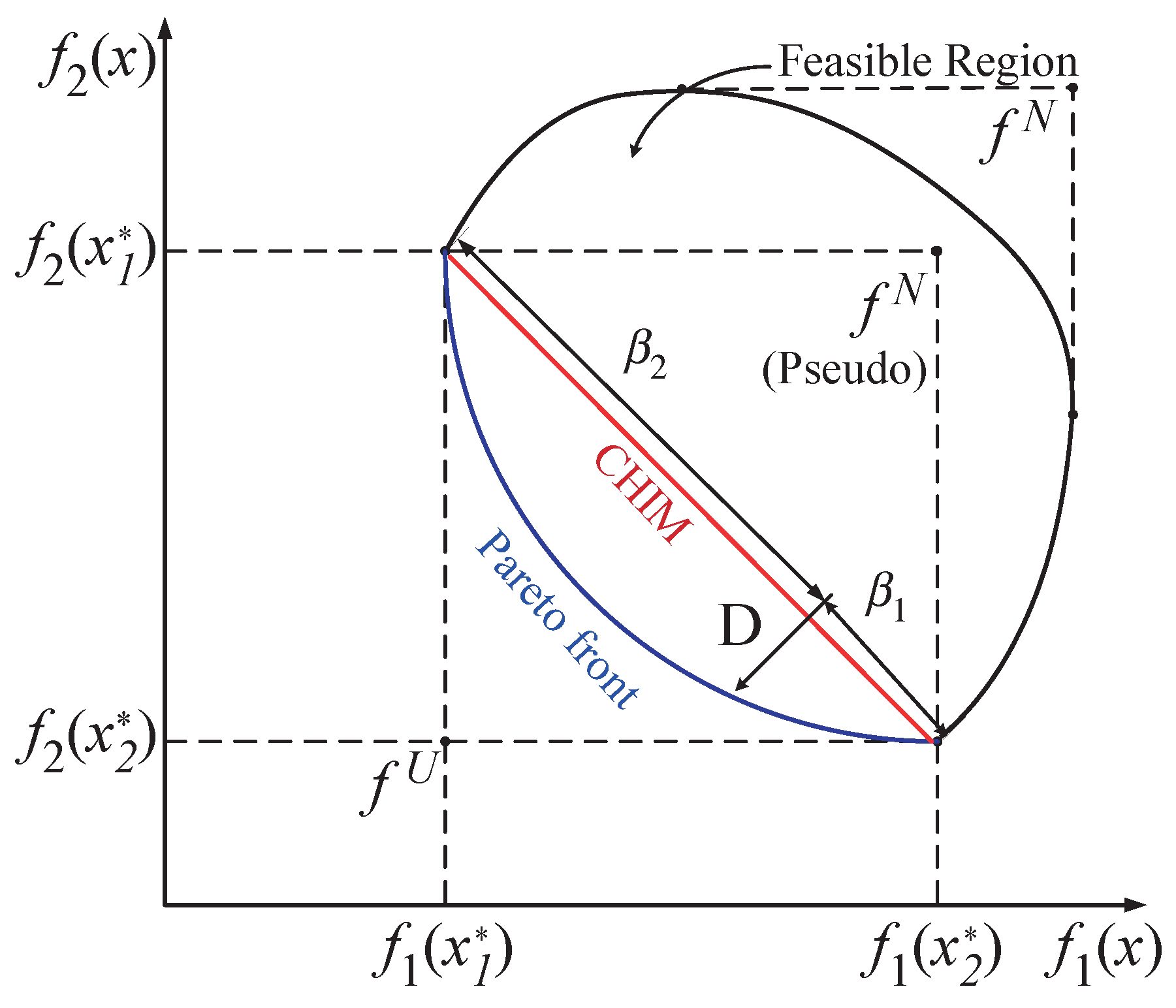
An arbitrary MOMP problem with two objective functions is depicted in Figure 2. The ith row of the payoff table consists of the obtained values for the ith objective function in which the maximum and the minimum values show the upper and lower limits of this objective function. These values will be used later to normalize the objective function space [41].
The utopia point is the point depicted in Figure 2 that corresponds to the best solution for all of the objectives simultaneously:
It generally lies outside of the feasible region. The nadir point is also shown in Figure 2. This point corresponds to the worst solution for all the objectives considered simultaneously, and is given by:
where
subject to . It generally lies outside of the feasible region as well. Therefore, a pseudo nadir point is defined as
As shown in Figure 2, the pseudo nadir point is the point with the worst design objective values of the anchor points within the feasible region. If the objective function values are not in the same numerical range, then they must be normalized to obtain a well represented set of Pareto solutions. The normalized value of the objective function (denoted as ) can be calculated using the utopia point and pseudo nadir point as follows:
After obtaining a normalized value for each objective function, a normalized payoff matrix can be constructed. The next step is to construct the shifted convex hull of the individual minima (CHIM), which are the convex combinations of each row of the payoff table. Any point in the normalized space on the CHIM line is expressed as:
Let be the unit normal to the CHIM towards the origin; then, represents the set of points on that normal. As a result, the original optimization problem is transformed into a set of parameterized single-objective optimization problems with the objective to maximize the distance between the utopia line and the Pareto surface. Finally, the closest intersection point of the normal and the boundary of feasible region to the origin is the global solution of the following sub-problem (NBI) [42]:
where . By solving Equation (24) for different values of , a point-wise approximation of the Pareto surface can be obtained.
3.2. Fuzzy Decision Making Method
The Pareto optimal solutions obtained are sorted by a fuzzy decision making method. The value of the functions in Equation (16) are computed for all of the saved solutions in the repository and consequently the solution with the highest value is considered as the best compromise solution [10]:
where is the weight factor for the kth objective function and M is the number of the non-dominant solutions. The weight factor can be selected by the operator to reflect operating preferences. The solution with the maximum membership function is the most preferred compromise solution based on the adopted weight factors and is selected as the best Pareto optimal solution to the problem.
4. Applications
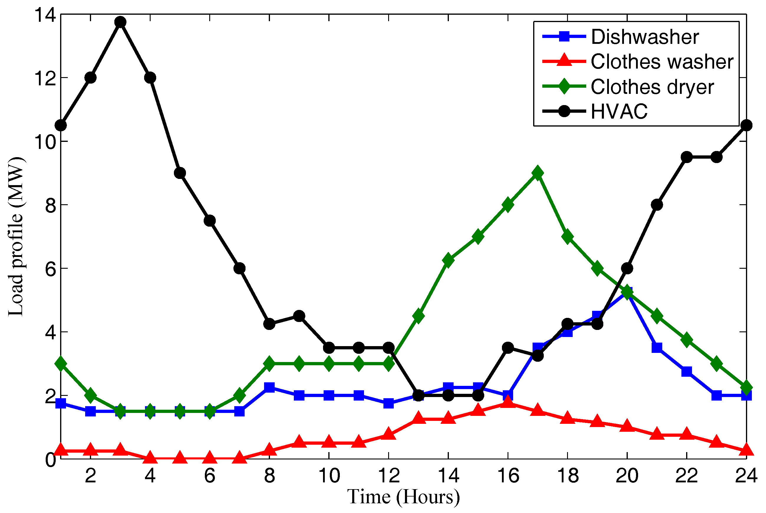
The proposed optimization process is validated on the six-generator test system detailed in [43]. The lower limit of all generators’ outputs has been changed in this study since it is not possible to turn off a generator in the DED problem and the total load must be less than or equal to the minimum generation limit of the system at each time interval. The optimization is performed using the General Algebraic Modeling System (GAMS), which is a high-level modeling system for mathematical programming and optimization. The coefficients for computing the generation cost and emissions, accompanied with the minimum and maximum generation limits for generators are given in Table 3. To implement the DSM, a load profile is specified for each load in the system. For each appliance, a normalized load profile based on the customer consumption pattern is defined. The total load at each time step is then computed as the product of the normalized load profile, the maximum power consumption of the appliance, and the number of participating DSM customers. The aggregated load profile across all consumers is shown in Figure 3. This load profile is for winter, so the peak load of the HVAC is during the evening. Load aggregators can gather the individual load profiles and responsive load values for all customers. Although similar appliance load profiles are assumed for all customers in this study, the general approach can be extended to include diverse load profiles for different customers.
To compare the effect of EVs and appliances on different objective functions, several scenarios including combinations of EVs and appliances as deferrable or nondeferrable loads are illustrated. The payoff table for the base case scenario (no deferrable loads) is given in Table 4. Table 5 gives the payoff table in the fully deferrable case. The payoff table values for varying ratios of EVs and loads will lie between these table values. Since the trend between the different objectives is inversely proportional, this implies that the combined objective functions form a Pareto front.
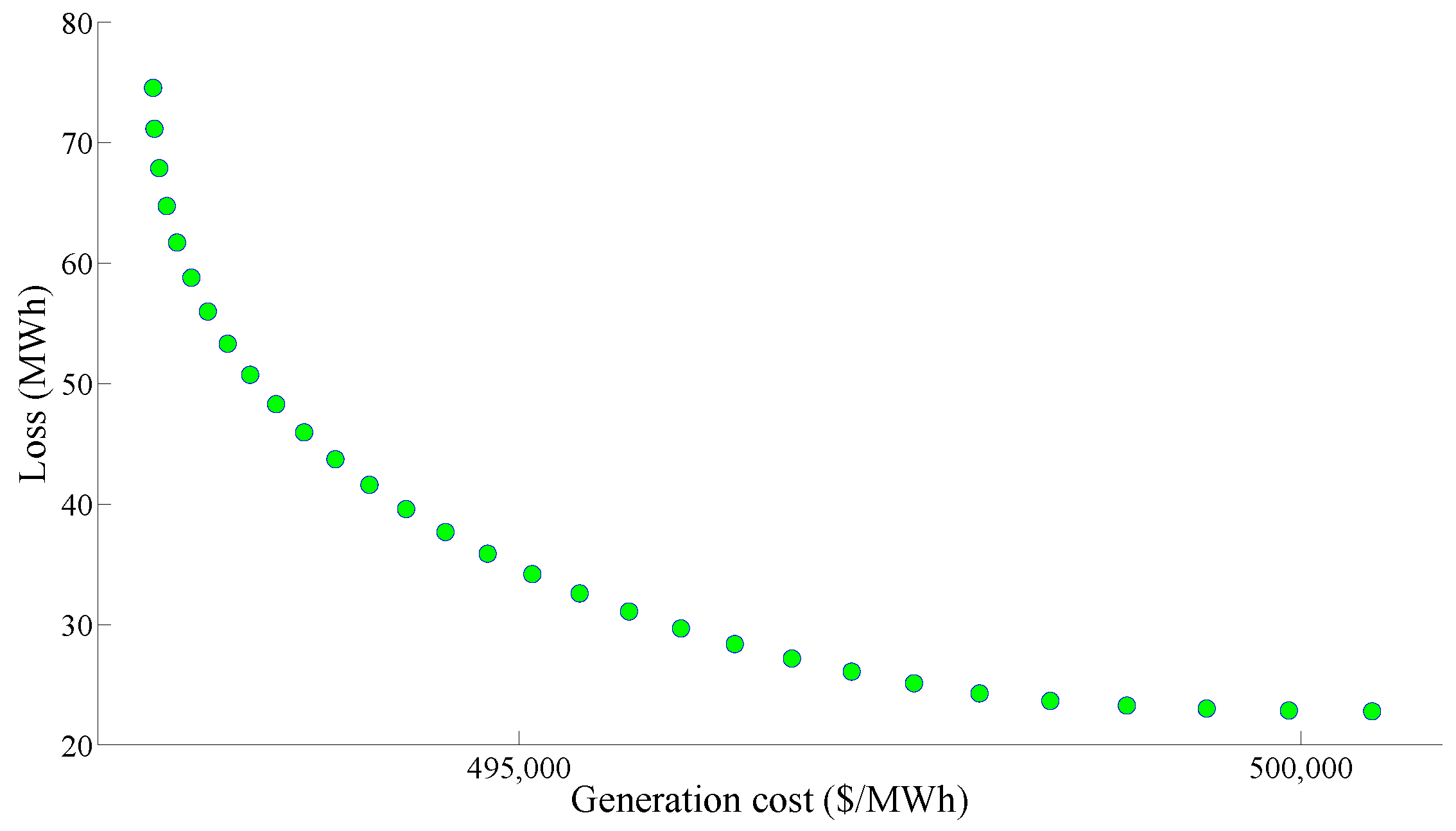
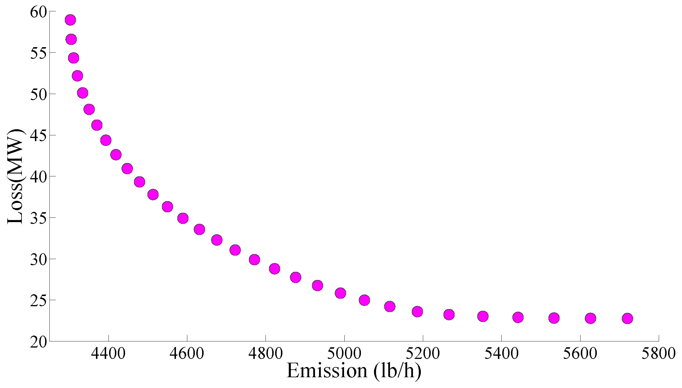
Since there are three objectives, three different combinations of objective functions can be obtained for two-dimensional Pareto fronts. These combinations are (a) generation costs and emissions, (b) generation costs and energy loss, and (c) energy loss and emissions. The Pareto fronts are shown in Figure 4, Figure 5 and Figure 6 for the first scenario.
Each Pareto optimal solution is a valid choice for the system, depending on the operating objectives. The best compromise solution for each multi-objective case is given in Table 6 and Table 7 for different scenarios. A compromise solution is one in which two of the three objectives are minimized. The power system operator can select the best compromise solution based on the policy preference. Different Pareto optimal solutions, instead of one optimal solution, can give the system operator and/or policy makers multiple choices, and assess the tradeoffs between different objectives.
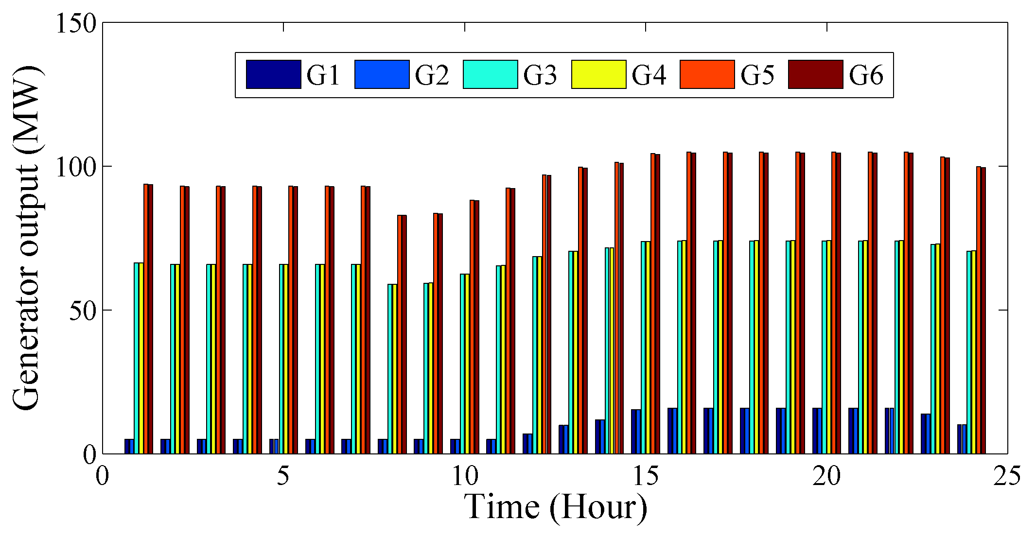
Given the same load profile, the generator outputs will be different depending on the optimization criteria. For example, Figure 7 shows the generator dispatch curves for the case in which the emissions criterion has greater emphasis than generation cost (Figure 8). When the dominant objective is to minimize emissions, the low emission units (G1–G3) produce more power throughout the day. However, when generation cost is the dominant factor, the low cost units (G4–G6) provide a much larger fraction of the overall generation.
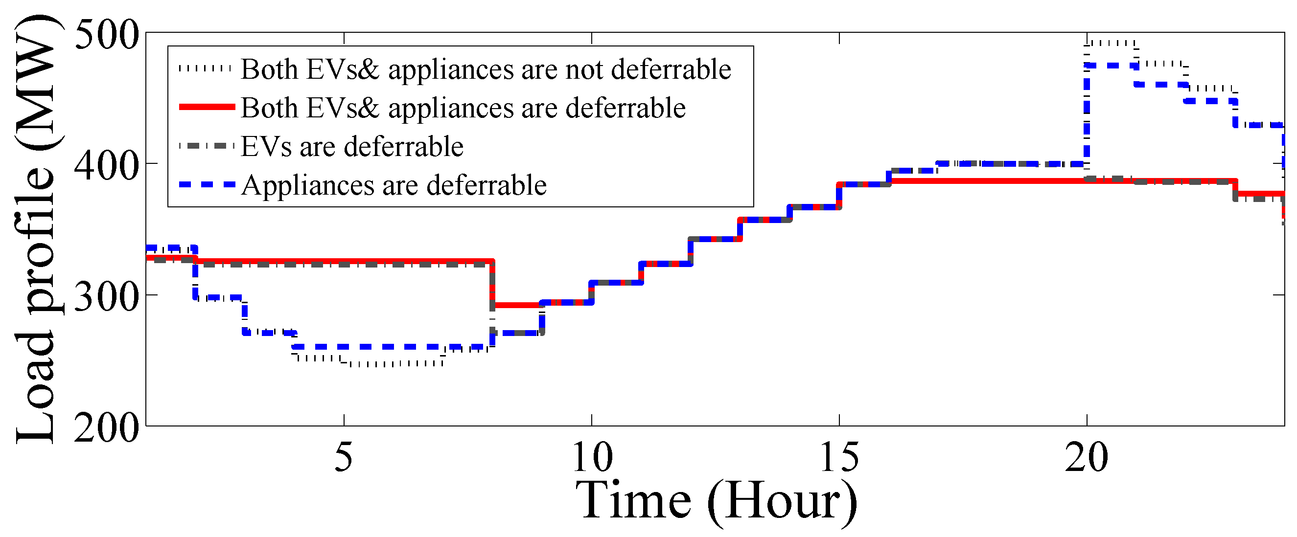
In all cases, however, the optimal results are obtained when there is a significant amount of deferrable loads. Figure 9 shows four cases:
- Base case (no deferrable loads)
- Only EV deferrable
- Only appliances deferrable
- Both EV and appliances deferrable
Figure 9 shows that the EV load dominates and its inclusion in the optimization yields improved results. Note when the EVs are not deferrable loads, there is a sharp peak at 7:00 p.m. due to the uncoordinated EV charging. By considering the EVs as deferrable loads, the load profile is significantly flattened and the severe peak is reduced. However, the total energy requirement over 24 h remains the same regardless of the load type (deferrable or nondeferrable).
5. Conclusions
In this paper, the normal boundary intersection method has been successfully implemented to solve the centralized multi-objective dynamic economic dispatch with demand side management of individual residential loads and electric vehicles. The proposed multi-objective optimization method minimizes the combination of generation costs, emissions, and energy loss while considering customers’ comfort by limiting acceptable delay times of household appliances. Applying the normal boundary intersection method provides a simple relation between the multiple objectives. It also facilitates finding the appropriate weighting factors with different orders of magnitudes for multiple objectives. A fuzzy decision making method has been implemented to find the best compromise solution based on the decision maker’s operating policy. This provides an effective tool to the power system operator to make decisions as needed. By combining these objectives, the solution is capable of incorporating both economics of the generation and transmission systems, and environmental effects into account. The proposed approach is simple in concept and easy to implement. In addition, it can be expanded easily to implement in larger case studies with more generators and households.
Acknowledgments
We would also like to show our gratitude to three “anonymous” reviewers for their so-called insights.
Author Contributions
All authors contributed equally to this work.
Conflicts of Interest
The authors declare no conflict of interest.
References
- Ma, J.; Chen, H.; Song, L.; Li, Y. Residential load scheduling in smart grid: A cost efficiency perspective. IEEE Trans. Smart Grid 2016, 7, 771–784. [Google Scholar] [CrossRef]
- Safdarian, A.; Degefa, M.Z.; Lehtonen, M.; Fotuhi-Firuzabad, M. Distribution network reliability improvements in presence of demand response. IET Gener. Transm. Distrib. 2014, 8, 2027–2035. [Google Scholar] [CrossRef]
- Smart Energy Demand Coalition. The Demand Response Snapshot the Reality for Demand Response Providers Working in Europe Today; Smart Energy Demand Coalition: Brussels, Belgium, 2011. [Google Scholar]
- Paulus, M.; Borggrefe, F. The potential of demand-side management in energy intensive industries for electricity markets in Germany. Appl. Energy 2011, 8, 432–441. [Google Scholar] [CrossRef]
- Hayes, J.B.; Hernando-Gil, I.; Collin, A.; Harrison, G.; Djokić, S. Optimal power flow for maximizing network benefits from demand-side management. IEEE Trans. Power Syst. 2014, 29, 1739–1747. [Google Scholar] [CrossRef]
- Huang, D.; Billinton, R. Effects of load sector demand side management applications in generating capacity adequacy assessment. IEEE Trans. Power Syst. 2012, 27, 335–343. [Google Scholar] [CrossRef]
- The U.S. General Services Administration Website. Available online: http://www.gsa.gov/portal/content/281581 (accessed on 15 September 2015).
- Orsi, F.; Muratori, M.; Rocco, M.; Colombo, E.; Rizzoni, G. A multi-dimensional well-to-wheels analysis of passenger vehicles in different regions: Primary energy consumption, CO2 emissions, and economic cost. Appl. Energy 2016, 169, 197–209. [Google Scholar] [CrossRef]
- Karabasoglu, O.; Michalek, J. Influence of driving patterns on life cycle cost and emissions of hybrid and plug-in electric vehicle power trains. Energy Policy 2013, 60, 445–461. [Google Scholar] [CrossRef]
- Narimani, M.R.; Azizipanah-Abarghooee, R.; Zoghdar-Moghadam-Shahrekohne, B.; Gholami, K. A novel approach to multi-objective optimal power flow by a new hybrid optimization algorithm considering generator constraints and multi-fuel type. Energy 2013, 49, 119–136. [Google Scholar] [CrossRef]
- Jubril, A.M.; Komolafe, O.A.; Alawode, K.O. Solving multi-objective economic dispatch problem via semidefinite programming. IEEE Trans. Power Syst. 2013, 28, 2056–2064. [Google Scholar] [CrossRef]
- Shao, S.; Pipattanasomporn, M.; Rahman, S. Demand response as a load shaping tool in an intelligent grid with electric vehicles. IEEE Trans. Smart Grid 2011, 2, 624. [Google Scholar] [CrossRef]
- Abdi, H.; Dehnavi, E.; Mohammadi, F. Dynamic economic dispatch problem integrated with demand response (DEDDR) considering nonlinear responsive load models. IEEE Trans. Smart Grid 2016. [Google Scholar] [CrossRef]
- Papavasiliou, A.; Oren, S.S. A stochastic unit commitment model for integrating renewable supply and demand response. In Proceedings of the 2012 IEEE Power and Energy Society General Meeting, San Diego, CA, USA, 22–26 July 2012. [Google Scholar] [CrossRef]
- Muratori, M.; Schuelke-Leech, B.; Rizzoni, G. Role of residential demand response in modern electricity markets. Renew. Sustain. Energ. Rev. 2014, 33, 546–553. [Google Scholar] [CrossRef]
- Narimani, M.R.; Nauert, P.J.; Joo, J.Y.; Crow, M.L. Reliability assesment of power system at the presence of demand side management. In Proceedings of the Power and Energy Conference at Illinois (PECI), Champaign, IL, USA, 19–20 February 2016. [Google Scholar] [CrossRef]
- Narimani, M.R.; Joo, J.Y.; Crow, M.L. The effect of demand response on distribution system operation. In Proceedings of the Power and Energy Conference at Illinois (PECI), Champaign, IL, USA, 20–21 February 2015. [Google Scholar] [CrossRef]
- Darabi, Z.; Ferdowsi, M.; Rahman, S. Aggregated impact of plug-in hybrid electric vehicles on electricity demand profile. IEEE Trans. Sustain. Energy 2011, 2, 501–508. [Google Scholar] [CrossRef]
- Shao, S.; Pipattanasomporn, M.; Rahman, S. Grid integration of electric vehicles and demand response with customer choice. IEEE Trans. Smart Grid 2012, 3, 543–550. [Google Scholar] [CrossRef]
- Sheikhi, A.; Bahrami, S.; Ranjbar, A.; Oraee, H. Strategic charging method for plugged in hybrid electric vehicles in smart grids: A game theoretic approach. Int. J. Electr. Power Energy Syst. 2013, 53, 499–506. [Google Scholar] [CrossRef]
- Wang, Z.; Wang, S. Grid power peak shaving and valley filling using vehicle-to-grid systems. IEEE Trans. Power Deliv. 2013, 28, 1822–1829. [Google Scholar] [CrossRef]
- Oviedo, R.M.; Fan, Z.; Gormus, S.; Kulkarni, P. A residential PHEV load coordination mechanism with renewable sources in smart grids. Int. J. Electr. Power Energy Syst. 2014, 55, 511–521. [Google Scholar] [CrossRef]
- López, M.A.; la Torre, S.D.; Martin, S.; Aguado, J.A. Demand-side management in smart grid operation considering electric vehicles load shifting and vehicle-to-grid support. Electr. Power Energy Syst. 2015, 64, 689–698. [Google Scholar] [CrossRef]
- Wu, D.; Aliprantis, D.C.; Gkritza, K. Electric energy and power consumption by light-duty plug-in electric vehicles. IEEE Trans. Power Syst. 2011, 26, 738–746. [Google Scholar] [CrossRef]
- Ashtari, A.; Bibeau, E.; Shahidinejad, S.; Molinski, T. PEV charging profile prediction and analysis based on vehicle usage data. IEEE Trans. Smart Grid 2012, 3, 341–350. [Google Scholar] [CrossRef]
- Rotering, N.; Ilic, M. Optimal charge control of plug-in hybrid electric vehicles in deregulated electricity markets. IEEE Trans. Power Syst. 2011, 26, 1021–1029. [Google Scholar] [CrossRef]
- Wu, D.; Aliprantis, D.C.; Ying, L. Load scheduling and dispatch for aggregators of plug-in electric vehicles. IEEE Trans. Smart Grid 2012, 3, 368–376. [Google Scholar] [CrossRef]
- Nguyen, D.T.; Le, L.B. Joint optimization of electric vehicle and home energy scheduling considering user comfort preference. IEEE Trans. Smart Grid 2014, 5, 188–199. [Google Scholar] [CrossRef]
- Paterakis, N.G.; Erdinc, O.; Bakirtzis, A.G.; Catalão, J.P.S. Optimal household appliances scheduling under day-ahead pricing and load-shaping demand response strategies. IEEE Trans. Ind. Inform. 2015, 11, 1509–1519. [Google Scholar] [CrossRef]
- Muratori, M.; Rizzoni, G. Residential demand response: Dynamic energy management and time-varying electricity pricing. IEEE Trans. Power Syst. 2016. [Google Scholar] [CrossRef]
- Mahmoodi, M.; Shamsi, P.; Fahimi, B. Economic dispatch of a hybrid microgrid with distributed energy storage. IEEE Trans. Smart Grid 2015, 6, 2607–2614. [Google Scholar] [CrossRef]
- Shamsi, P.; Xie, H.; Longe, A.; Joo, J.Y. Economic dispatch for an agent-based community microgrid. IEEE Trans. Smart Grid 2016, 7, 2317–2324. [Google Scholar] [CrossRef]
- Taneja, J.; Lutz, K.; Culler, D. The Impact of Flexible Loads in Increasingly Renewable Grids. In Proceedings of the IEEE International Conference on Smart Grid Communications, Vancouver, BC, Canada, 21–24 October 2013. [Google Scholar]
- Safdarian, A.; Fotuhi-Firuzabad, M.; Lehtonen, M. Benefits of demand response on operation of distribution networks: A case study. IEEE Syst. J. 2016, 10, 189–197. [Google Scholar] [CrossRef]
- Narimani, M.R.; Joo, J.Y.; Crow, M.L. Dynamic economic dispatch with demand side management of individual residential loads. In Proceedings of the North American Power Symposium, Charlotte, NC, USA, 4–6 October 2015. [Google Scholar] [CrossRef]
- Bai, X.; Qiao, W. Robust optimization for bidirectional dispatch coordination of large-scale V2G. IEEE Trans. Smart Grid 2015, 6, 1944–1954. [Google Scholar] [CrossRef]
- Wang, Y.; Wang, B.; Chu, C.C.; Pota, H.; Gadh, R. Energy management for a commercial building microgrid with stationary and mobile battery storage. Energy Build. 2016, 116, 141–150. [Google Scholar] [CrossRef]
- Maigha; Crow, M.L. Economic scheduling of residential plug-in (hybrid) electric vehicle (PHEV) charging. Energies 2014, 7, 1876–1898. [Google Scholar] [CrossRef]
- Deb, K. Multiobjective Optimization Using Evolutionary Algorithms; Wiley: New York, NY, USA, 2001. [Google Scholar]
- Ahmadi, A.; Moghimi, H.; Nezhad, A.E.; Agelidis, V.G.; Sharaf, A.M. Multi-objective economic emission dispatch considering combined heat and power by normal boundary intersection method. Electr. Power Syst. Res. 2015, 129, 32–43. [Google Scholar] [CrossRef]
- Vahidinasab, V.; Jadid, S. Normal boundary intersection method for suppliers’ strategic bidding in electricity markets: An environmental/economic approach. Energy Convers. Manag. 2010, 51, 1111–1119. [Google Scholar] [CrossRef]
- Das, I.; Dennis, J.E. Normal boundary intersection: A new method for generating the Pareto surface in nonlinear multicriteria optimization problems. SIAM J. Optim. 1998, 8, 631–657. [Google Scholar] [CrossRef]
- Roy, P.K.; Bhui, S. Multi-objective quasi-oppositional teaching learning based optimization for economic emission load dispatch problem. Electr. Power Energy Syst. 2013, 53, 937–948. [Google Scholar] [CrossRef]
Figure 1.
Average driving distances (miles).

Figure 2.
Normal boundary intersection (NBI) method for obtaining Pareto front.

Figure 3.
Load profiles of different deferrable loads.

Figure 4.
Pareto front for generation cost and emission objective functions when both EVs and appliances are deferrable.
Figure 4.
Pareto front for generation cost and emission objective functions when both EVs and appliances are deferrable.
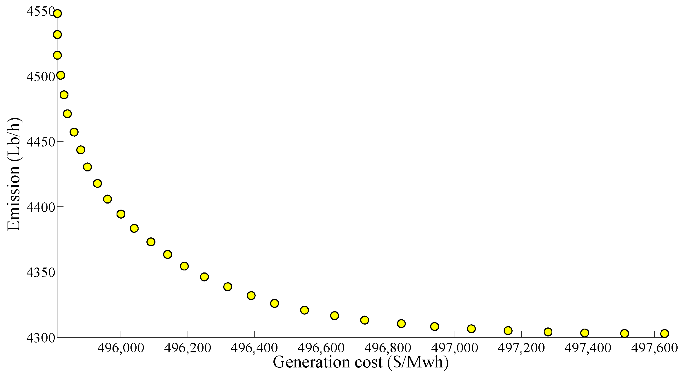
Figure 5.
Pareto front for generation cost and energy loss objective functions when both EVs and appliances are deferrable.
Figure 5.
Pareto front for generation cost and energy loss objective functions when both EVs and appliances are deferrable.

Figure 6.
Pareto front for energy loss and emission objective functions when both EVs and appliances are deferrable.
Figure 6.
Pareto front for energy loss and emission objective functions when both EVs and appliances are deferrable.

Figure 7.
Generator outputs for best emission and worst generation cost.

Figure 8.
Generator outputs for best generation cost and worst emission.
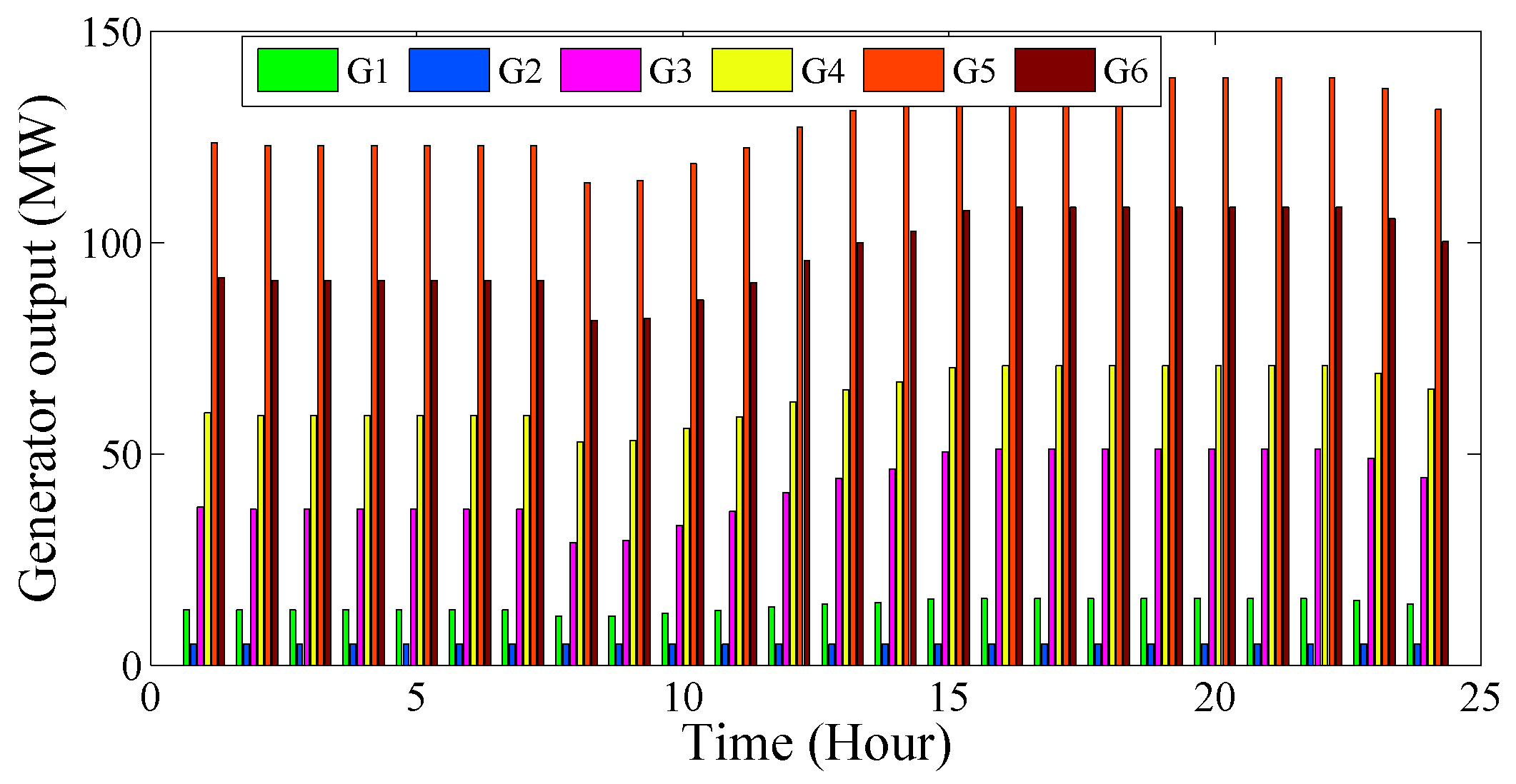
Figure 9.
Total load profiles for different scenarios.

Table 1.
Acceptable delay times (ADT) for different appliances.
| Appliances | ADT (h) |
|---|---|
| Heating, ventilation, and air-conditioning (HVAC) | 2 |
| Clothes washer | 3 |
| Clothes dryer | 3 |
| Dishwasher | 4 |
Table 2.
Battery characteristics.
| Battery Capacity (kWh) | All Electric Range |
|---|---|
| 11 | 30 |
| 12 | 40 |
| 16 | 70 |
| 18 | 80 |
| 24 | 100 |
Table 3.
Generator coefficients.
| Generator Information | G1 | G2 | G3 | G4 | G5 | G6 |
|---|---|---|---|---|---|---|
| a | 0.153 | 0.106 | 0.036 | 0.028 | 0.018 | 0.021 |
| b | 38.539 | 46.159 | 38.306 | 40.397 | 38.270 | 36.328 |
| c | 756.8 | 451.3 | 1243.5 | 1050.0 | 1356.7 | 1658.6 |
| 5 | 5 | 20 | 20 | 50 | 50 | |
| 125 | 150 | 210 | 225 | 325 | 325 | |
| 13.859 | 13.859 | 40.267 | 40.267 | 42.896 | 42.896 | |
| 0.328 | 0.3278 | |||||
| 0.0042 | 0.0042 | 0.0068 | 0.0068 | 0.0046 | 0.0046 |
Table 4.
Payoff table when neither appliances nor electric vehicles (EVs) are deferrable loads (base case).
Table 4.
Payoff table when neither appliances nor electric vehicles (EVs) are deferrable loads (base case).
| Objective Functions | Generation Cost | Energy Loss | Emission |
|---|---|---|---|
| ($/MWh) | (MWh) | (lb/h) | |
| Generation Cost | 496,504 | 76.5 | 4681 |
| Energy Loss | 517,013 | 23.3 | 5934 |
| Emissions | 498,929 | 58.2 | 4408 |
Table 5.
Payoff table for objective functions when both EVs and appliances are deferrable loads.
| Objective Functions | Generation Cost | Energy Loss | Emission |
|---|---|---|---|
| ($/MWh) | (MWh) | (lb/h) | |
| Generation Cost | 495,805 | 74.5 | 4548 |
| Energy Loss | 515,230 | 22.8 | 5720 |
| Emissions | 497,632 | 59.0 | 4303 |
Table 6.
Best compromise solutions for different objective functions (base case).
| Objective Functions | Best Compromise Solution |
|---|---|
| Generation Cost and Emissions | 497,390 ($/MWh), 4436 (lb/h) |
| Generation Cost and Energy Loss | 502,340 ($/MWh), 34.9 (MWh) |
| Emissions and Energy Loss | 4848 (lb/h), 31.0 (MWh) |
Table 7.
Best compromise solutions for different objective functions when both EVs and appliances are deferrable.
Table 7.
Best compromise solutions for different objective functions when both EVs and appliances are deferrable.
| Objective Functions | Best Compromise Solution |
|---|---|
| Generation Cost and Emissions | 496,470 ($/MWh), 4339 (lb/h) |
| Generation Cost and Energy Loss | 501,380 ($/MWh), 34.2 (MWh) |
| Emissions and Energy Loss | 4722 (lb/h), 31.1 (MWh) |
© 2017 by the authors. Licensee MDPI, Basel, Switzerland. This article is an open access article distributed under the terms and conditions of the Creative Commons Attribution (CC BY) license (http://creativecommons.org/licenses/by/4.0/).
Share and Cite
MDPI and ACS Style
Narimani, M.R.; Maigha; Joo, J.-Y.; Crow, M. Multi-Objective Dynamic Economic Dispatch with Demand Side Management of Residential Loads and Electric Vehicles. Energies 2017, 10, 624. https://doi.org/10.3390/en10050624
AMA Style
Narimani MR, Maigha, Joo J-Y, Crow M. Multi-Objective Dynamic Economic Dispatch with Demand Side Management of Residential Loads and Electric Vehicles. Energies. 2017; 10(5):624. https://doi.org/10.3390/en10050624
Chicago/Turabian StyleNarimani, Mohammad Rasoul, Maigha, Jhi-Young Joo, and Mariesa Crow. 2017. "Multi-Objective Dynamic Economic Dispatch with Demand Side Management of Residential Loads and Electric Vehicles" Energies 10, no. 5: 624. https://doi.org/10.3390/en10050624
Note that from the first issue of 2016, this journal uses article numbers instead of page numbers. See further details here.