Using SF₆ Decomposed Component Analysis for the Diagnosis of Partial Discharge Severity Initiated by Free Metal Particle Defect

Abstract

The decomposition characteristics of a SF₆ gas-insulated medium were used to diagnose the partial discharge (PD) severity in DC gas-insulated equipment (DC-GIE). First, the PD characteristics of the whole process were studied from the initial PD to the breakdown initiated by a free metal particle defect. The average discharge magnitude in a second was used to characterize the PD severity and the PD was divided into three levels: mild PD, medium PD, and dangerous PD. Second, two kinds of voltage in each of the above PD levels were selected for the decomposition experiments of SF₆. Results show that the negative DC-PD in these six experiments decomposes the SF₆ gas and generates five stable decomposed components, namely, CF₄, CO₂, SO₂F₂, SOF₂, and SO₂. The concentrations and concentration ratios of the SF₆ decomposed components can be associated with the PD severity. A minimum-redundancy-maximum-relevance (mRMR)-based feature selection algorithm was used to sort the concentrations and concentration ratios of the SF₆ decomposed components. Back propagation neural network (BPNN) and support vector machine (SVM) algorithms were used to diagnose the PD severity. The use of C(CO₂)/CT₁, C(CF₄)/C(SO₂), C(CO₂)/C(SOF₂), and C(CF₄)/C(CO₂) shows good performance in diagnosing PD severity. This finding serves as a foundation in using the SF₆ decomposed component analysis (DCA) method to diagnose the insulation faults in DC-GIE and assess its insulation status.

1. Introduction

SF₆ possesses excellent insulating and arc-extinguishing performance and is widely used as a medium in gas-insulated equipment (GIE) because of its ability to greatly reduce the equipment size and improve system reliability [1,2,3,4,5]. DC-GIE received much attention due to the rapid development of high-voltage DC (HVDC) transmission and flexible HVDC technologies [6,7,8,9,10,11]. However, when partial discharge (PD) occurs inside the equipment, this phenomenon can decompose SF₆ and generate a series of low-fluorine sulfides (such as SF₅, SF₄, SF₃, and SF₂). These low-fluorine sulfides then react with the trace moisture and oxygen that inevitably exist in the equipment, thus generating some stable decomposition products, such as SO₂F₂, SOF₂, SO₂, CF₄, CO₂, HF, and H₂S and resulting in the insulation performance degradation of SF₆ [12,13,14,15,16,17]. Using SF₆ decomposed component analysis (DCA) to diagnose the insulation faults in DC-GIE and assess its insulation status can effectively avoid the complex electromagnetic interference in the substation; this method has recently become a popular topic for researchers around the world [18,19,20,21].

The decomposition characteristics of SF₆ under four typical PD types in GIE were studied based on the DCA method [22,23,24,25], and the three-ratio method, which was similar to oil chromatographic analysis, was proposed for the recognition of the PD type. In addition to determining the discharge type, the discharge severity should be defined when assessing the insulation status of GIE. Parameters, such as apparent discharge magnitude, discharge repetition rate, and discharge time interval measured by pulse current method (PCM) are important features that characterize the discharge severity under DC conditions. However, PCM cannot be used to diagnose discharge severity in the field due to the multi-point grounding of real GIE. A large number of studies [22,23,24,25,26,27] reported the close relationships between the decomposition characteristics of the SF₆ gas-insulated medium and the type, energy consumption, and development trend of PD in GIE. Therefore, the SF₆ DCA method can be used to diagnose the PD severity in DC-GIE; however, no relevant study has been conducted about this topic.

This research develops a ball-bowl electrode to simulate the free metal particle insulation defect in DC-GIE and studies the PD characteristics of the whole process from the initial PD to the breakdown by using the built experimental platform. Based on the PD characteristics, the PD initiated by free metal particles is divided into three levels: mild PD, medium PD, and dangerous PD. Two kinds of voltage in each of the above PD levels are selected for the decomposition experiments of SF₆, and the decomposed components are measured by gas chromatography/mass spectrometry (GC/MS). A minimum-redundancy-maximum-relevance (mRMR)-based feature selection algorithm [28,29,30,31,32,33] is used to sort the concentrations and concentration ratios of SF₆ decomposed components. Back propagation neural network (BPNN) [24,34,35,36,37,38,39,40,41] and support vector machine (SVM) [41,42,43,44,45,46,47] algorithms are used to diagnose the PD severity. This research proposes the feature subset that can effectively characterize the PD severity and serves as a foundation for using the DCA method to diagnose the insulation faults in DC-GIE and assess its insulation status.

2. Experiment

2.1. Experimental Platform

The experimental platform of SF₆ decomposition under negative DC-PD is shown in Figure 1, which mainly includes four parts: the HVDC supply system, PD gas chamber, decomposed component detection system, and PD signal detection system.

The HVDC supply system mainly includes: voltage regulator (T₁: 0–380 V), testing transformer (T₂: 50 kVA/100 kV), HV silicon stack (D_s: 100 kV/5 A), filter capacitor (C_f: 0.2 μF), protective resistor (R₁: 20 kΩ, R₂: 20 kΩ), capacitive voltage divider (C_v, capacitance of HV arm: 500 pF, capacitance of low-voltage (LV) arm: 0.5 μF), and resistive voltage divider (R_v, resistance of HV arm: 220 MΩ, resistance of LV arm: 22 kΩ).

The PD gas chamber is made of stainless steel, has volume of 60 L that can withstand 0.7 MPa gas pressure, and has a good sealing performance as shown in Figure 2.

The decomposed component detection system uses the GC/MS (Shimadzu QP-2010Ultra, precision: 0.01 ppm, accuracy: ±10%, Shimadzu, Kyoto, Japan) to quantitatively measure the sample gas. The working conditions of GC/MS are as follows: injection port temperature: 220 °C; sample volume: 1 mL; total flow: 16.2 mL/min; pillar flow: 1.20 mL/min; linear velocity: 28.0 cm/s; blow flow: 3.0 mL/min; split ratio 10:1; connecter temperature: 220 °C; ion source: 200 °C; and ionization pattern: electron impact. The external standard method is used for the quantitative indication of SF₆ decomposed components [22]. The retention time and absolute calibration factor K_i of CF₄, CO₂, SO₂F₂, SOF₂, and SO₂ are shown in

Table 1. The retention time and absolute calibration factor K_i.

Decomposed Components	Retention Time/s	Ki/10−5	R2
CF4	4.320	2.838	0.999
CO2	4.815	2.525	0.999
SO2F2	5.055	2.670	0.999
SOF2	5.425	3.575	0.999
SO2	7.095	2.472	0.999

.

In the PD signal detection system, the coupling capacitor (C_k) is used to extract the pulse current, and the non-inductive impedance (Z_m) is used to convert this pulse current into a pulse voltage, which is sent to the digital storage oscilloscope (DSO, WavePro 7100XL, Lecroy, New York, NY, USA, analogue band: 1 GHz, sampling rate: 20 GHz, memory depth: 48 MB). This research uses the PD calibration circuit recommended by IEC 60270:2000 to calibrate the PD magnitude [48], and the calibration curve obtained is shown in Figure 3.

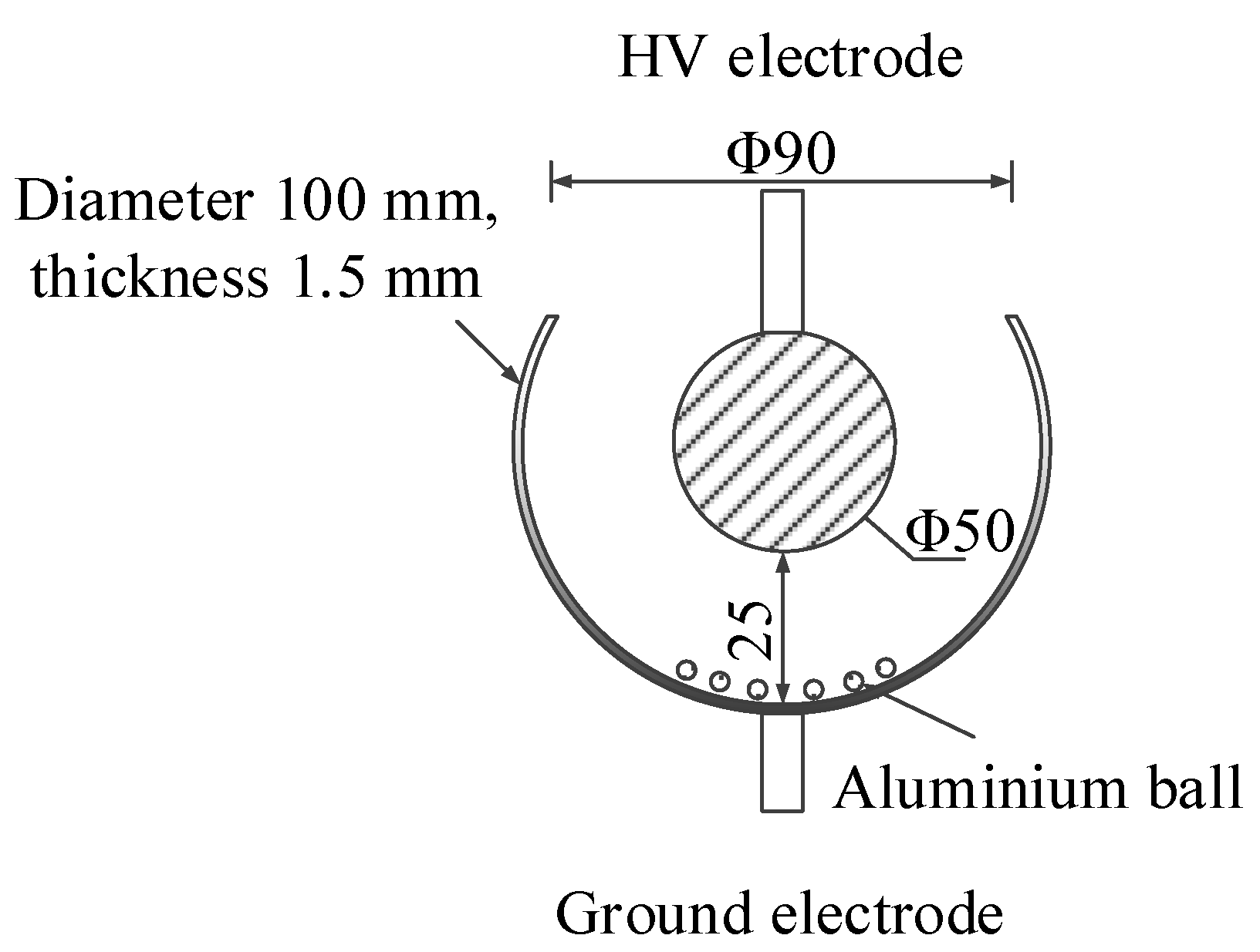
2.2. Insulation Defect Model

Many types of insulation defects might occur in DC-GIE; however, the most common defect is free metal particles, which is metal powder that can move freely in a cavity. As shown in Figure 4, a ball-bowl electrode, which consists of a ball electrode, a bowl electrode, and 20 aluminum balls (mass fraction of C element: 0.88%), is developed to simulate the particle defect. The ball and bowl electrodes form a concentric sphere structure and are made of stainless steel (mass fraction of C element: 0.10%). The diameter of the ball electrode is 50 mm. A hollow sphere is cut to obtain the bowl electrode with a thickness of 1.5 mm. The diameters of the hollow sphere, circular incision, and aluminum ball are 100, 90, and 3 mm, respectively.

2.3. Experimental Method

All experiments are conducted under the same conditions: the laboratory temperature and relative humidity are maintained at 20 °C and 50%, respectively. The purity of new SF₆ gas is 99.9995%. The specific experimental steps are listed as follows:

(1)

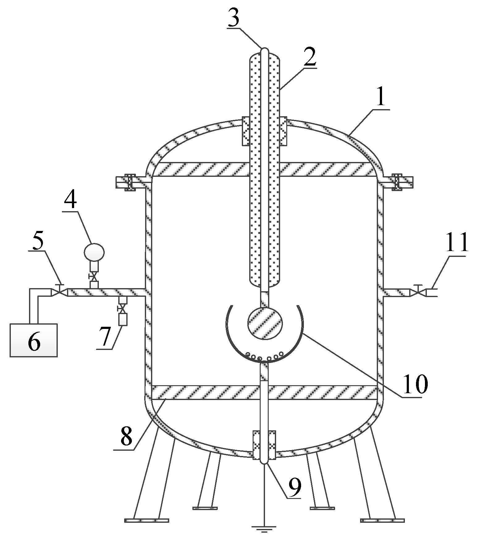
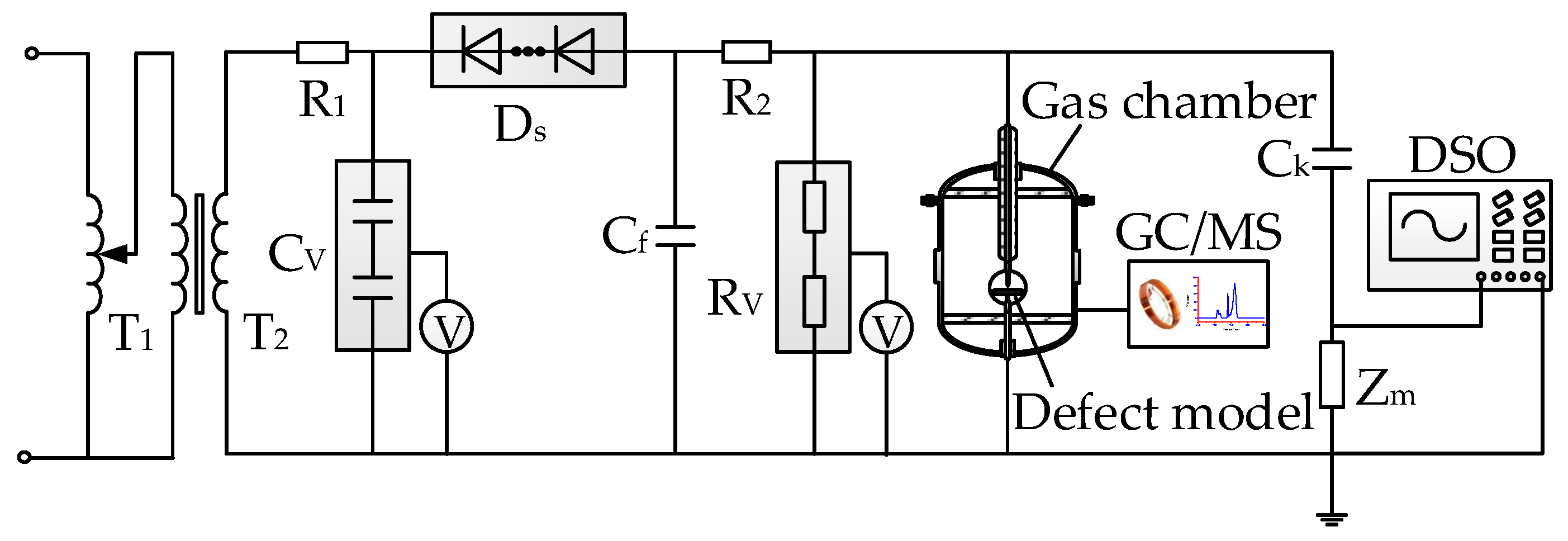
The experimental platform is connected as shown in Figure 1. The absolute alcohol is used to scrub the insulation defect model and the inner wall of the PD gas chamber. The chamber is set aside for 1 h to completely volatize the alcohol. The defect model is placed in the gas chamber.

(2)

The PD gas chamber is vacuumed and then filled with 0.3 MPa new SF₆ gas. This process is repeated several times for purification. A GE600 mirror dew-point meter is used to measure the H₂O concentration, and a GPR-1200 ppm portable oxygen analyzer is used to measure the O₂ concentration in the chamber. The concentrations of H₂O and O₂ are ensured to satisfy the industrial standard of DL/T 596-1996 [49].

(3)

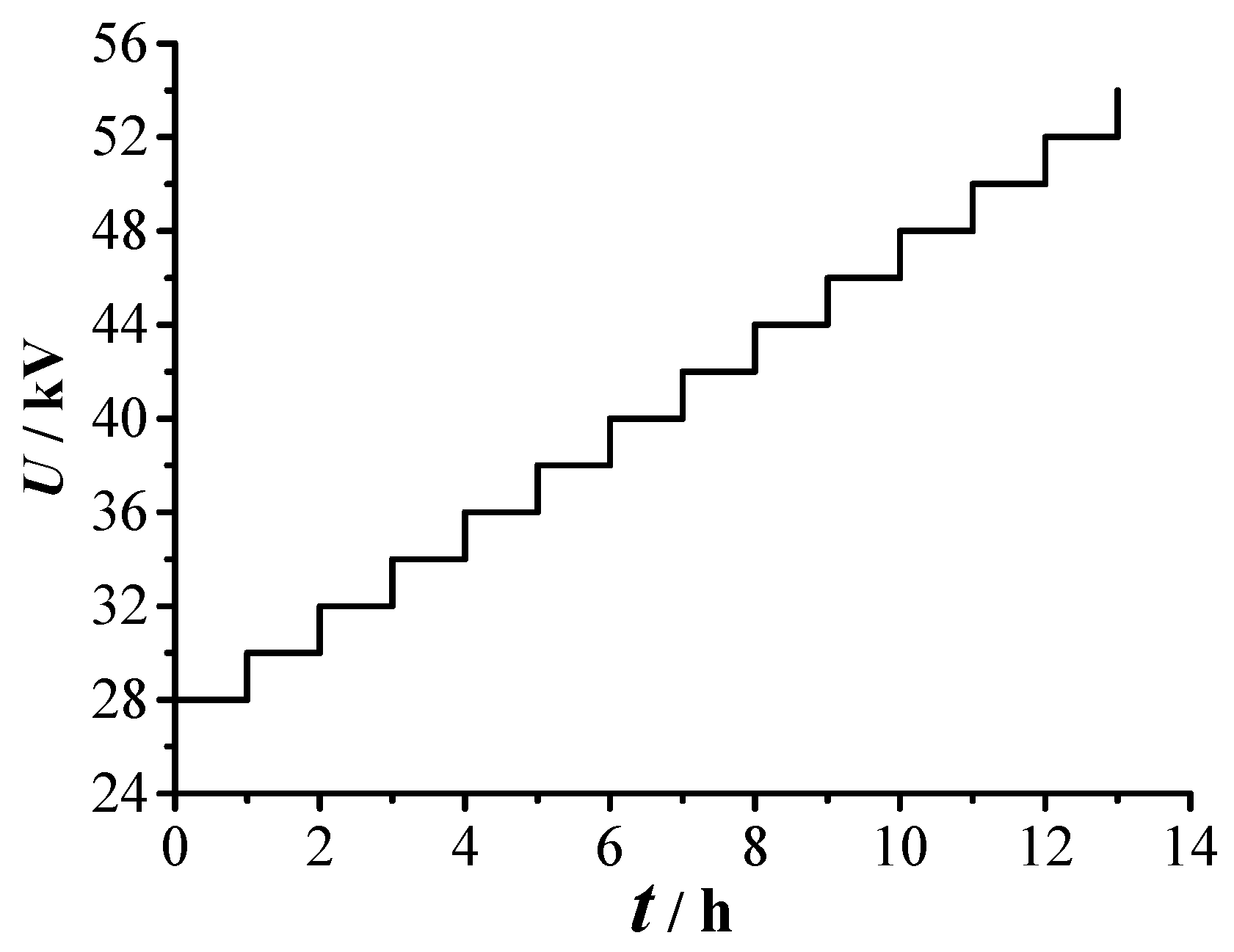
The voltage applied is gradually increased to the required experimental voltage. The decomposition experiment of SF₆ is conducted for 96 h under each voltage value. The SF₆ decomposed components are collected every 12 h. GC/MS is used to measure the concentrations of the decomposed components, and DSO is used to display and store the PD signals.

3. Experimental Results

3.1. PD Severity Division

The initial PD voltage U_g of the equipment without the particle defect is 82.2 kV. After placing the defect in the gas chamber, the initial PD voltage U₀ and breakdown voltage U_b of the equipment are 27.5 and 53.8 kV, respectively. The PD experiment is conducted under the grading voltage (Figure 5) to study the PD characteristics of the whole process when the applied voltage is increased. A total of 100 groups of PD signals are collected under each voltage value, and the PD parameters are obtained by averaging the three repeated experiments to ensure that the experimental results are statistically significant. Among the PD parameters, the discharge amplitude and repetition rate are two important features that can characterize the PD severity. The average discharge magnitude in a second (Q_sec, unit: pC/s) is selected as the characteristic quantity of PD severity to comprehensively consider the influence of these two parameters on PD development [26,27]. Q_sec is calculated using Equation (1).

$$Q_{\mathrm{s}\mathrm{e}\mathrm{c}}=Q_{\mathrm{a}\mathrm{v}\mathrm{g}}\times N$$

(1)

where Q_avg is the average charge of all single pulse within the measuring time (unit: pC/pulse) and N is the PD repetition rate (unit: pulse/s).

The change curves of three PD parameters with voltage applied are shown in Figure 6. With increasing experimental voltage, Q_sec gradually increases from about 3000 to 178,000 pC/s. This paper divides the PD into three levels according to Q_sec (region I: mild PD, region II: medium PD, and region III: dangerous PD) as shown in

Table 2. Division of PD severity.

Qsec (pC/s)	U/kV	Region	PD Severity
0–6 × 104	28, 30, 32, 34, 36, 38	I	Mild PD
6 × 104–12 × 104	40, 42, 44	II	Medium PD
12 × 104–18 × 104	46, 48, 50, 52	III	Dangerous PD

. When the applied voltage is slightly higher than the initial PD voltage (initial PD stage: from 28 to 30 kV), Q_avg and N grow rapidly. If the initial PD stage is excluded from region I, then the average growth rate of N in region II is the largest (reaching 35.58 pulse/(s·kV)), and the average growth rate of Q_avg in region III is the largest (reaching 9.99 pC/(pulse·kV)). Therefore, the division method for PD severity is reasonable.

3.2. Analysis of SF₆ Decomposed Characteristics

Considering the limitations of the experimental conditions, two kinds of voltage in each abovementioned PD level are used for the decomposition experiment of SF₆. The total concentration of SF₆ decomposed components is small when the applied voltage is less than 30 kV. Therefore, six kinds of voltage (mild PD: 32, 36 kV; medium PD: 40, 44 kV; and dangerous PD: 48, 52 kV) are used for the experiments, and SF₆ decomposed characteristics are used to diagnose the PD severity. Experimental results show that five stable decomposed components, namely, CF₄, CO₂, SO₂F₂, SOF₂, and SO₂ are detected under each voltage value.

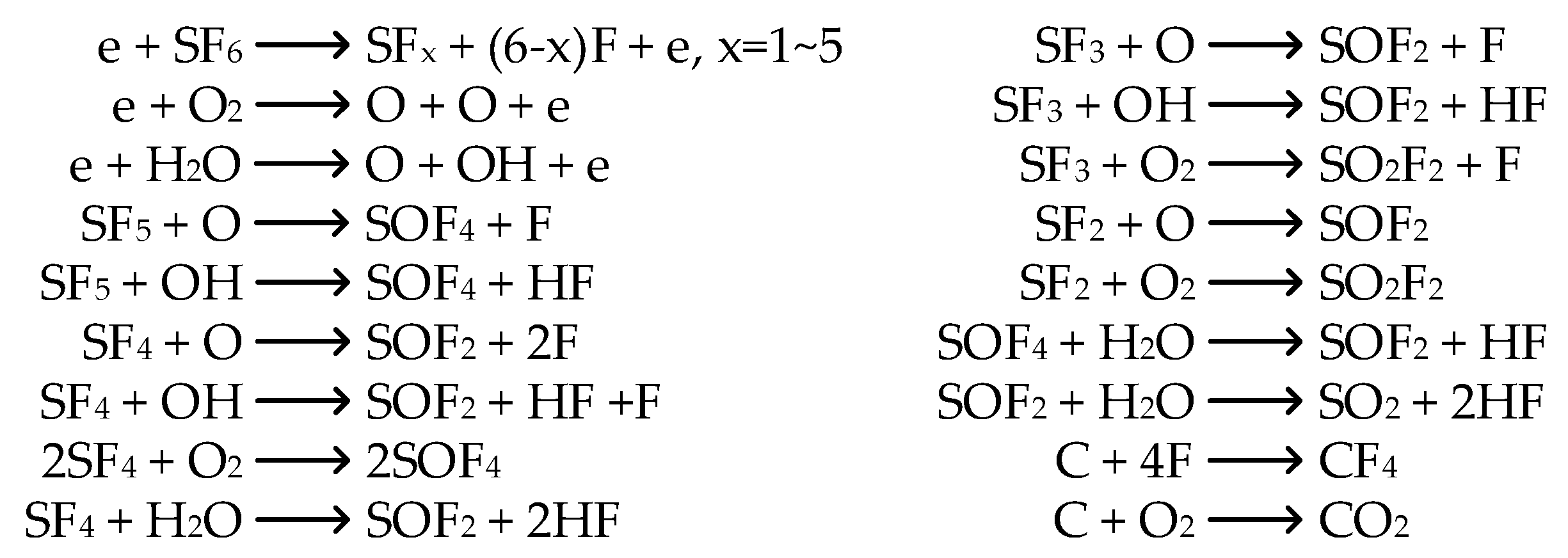
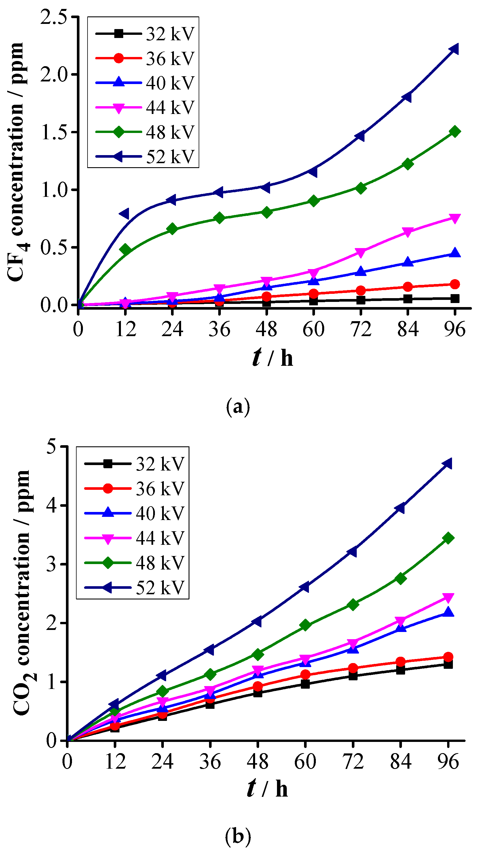
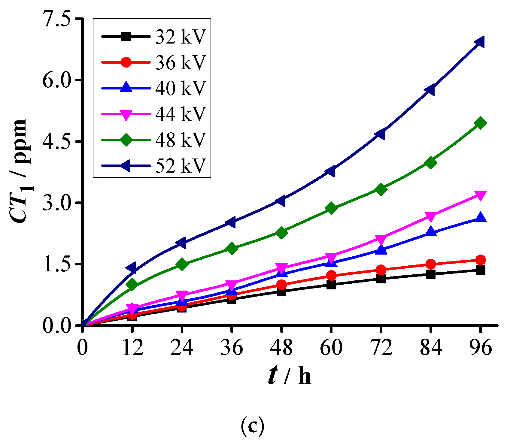
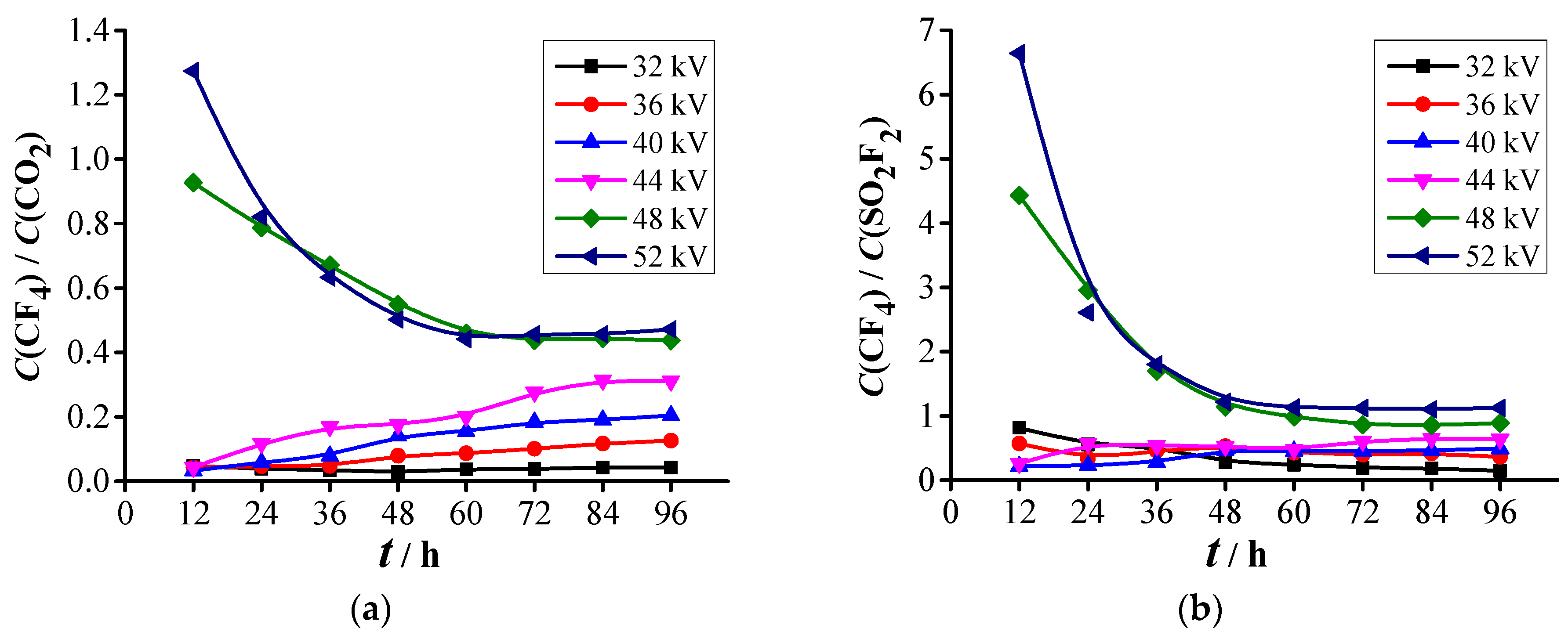
3.2.1. Formation Characteristics of Carbon-Containing Components

The formation process of SF₆ decomposed components is shown in Figure 7 [24]. CF₄ is generated through the reaction of C atom with F atom. Under the effect of the electric field, the charged particles hit the surface of the stainless-steel electrodes and aluminum balls to release the C atoms, as well as hit the SF₆ molecules and break six S-F bonds to generate F atoms; both processes require high-energy collision ionization. By calculation [50], the energy of the charged particle is low when the voltage U ≤ 36 kV [26,27]. Therefore, when the voltage U ≤ 36 kV, only a small amount of C atoms and F atoms are generated from the collision ionization, and the CF₄ concentration increases slowly with time (Figure 8a). When the voltage U > 36 kV, the energy of the charged particle increases. Thus, the growth rate of CF₄ concentration also increases. In particular, the CF₄ concentration quickly increases after 60 h. Limited F atoms are produced within 60 h. Thus, these limited F atoms have high possibility of reacting with metal and generate metal fluoride as compared with C atoms. This phenomenon limits the formation of CF₄ to some extent. After 60 h, the formed C atoms and F atoms continue to accumulate, and the excess F atoms will react with the C atoms and produce CF₄. Thus, the growth rate of CF₄ concentration accelerates.

The C atoms react with O₂ to generate CO₂. As shown in Figure 8b, the CO₂ concentration shows a saturated growth trend after 60 h when the voltage U ≤ 36 kV. The C atoms in the surface of the stainless-steel electrodes and aluminum balls are gradually inspired with time, and only high-energy charged particles can inspire the C atoms in the deep layer. However, the energy of the charged particle at this stage is low, which inhibits the formation of CO₂. Thus, the CO₂ concentration presents a saturated growth trend. When the voltage U > 36 kV, the CO₂ concentration shows an approximately linear growth trend with time, which indicates that the charged particles at this stage can stimulate the deeper C atoms under the surface of the stainless-steel electrodes and aluminum balls.

No organic insulating material exists near the PD area initiated by the particle defect. Thus, the concentration of (CF₄ + CO₂) can be used to characterize the amount of the carbon-containing metal involved in the reactions. CT₁ is defined to characterize the deterioration degree of carbon-containing metal in DC-GIE, and its formula is as follows:

$$C{T}_1=C(\mathrm{C}{\mathrm{F}}_4)+C(\mathrm{C}{\mathrm{O}}_2)$$

(2)

where C(CF₄) and C(CO₂) represent the concentrations of CF₄ and CO₂ (unit: ppm), respectively. As shown in Figure 8c, when mild PD (32 and 36 kV) occurs, CT₁ shows a saturated growth trend at the end of the experiment. When medium PD (40 and 44 kV) occurs, CT₁ presents an approximately linear growth trend with time. When dangerous PD (48 and 52 kV) occurs, CT₁ shows an approximately “J” growth trend at the end of the experiment. The change curves of CT₁ differ under three different PD levels. Thus, CT₁ can be associated with the PD severity.

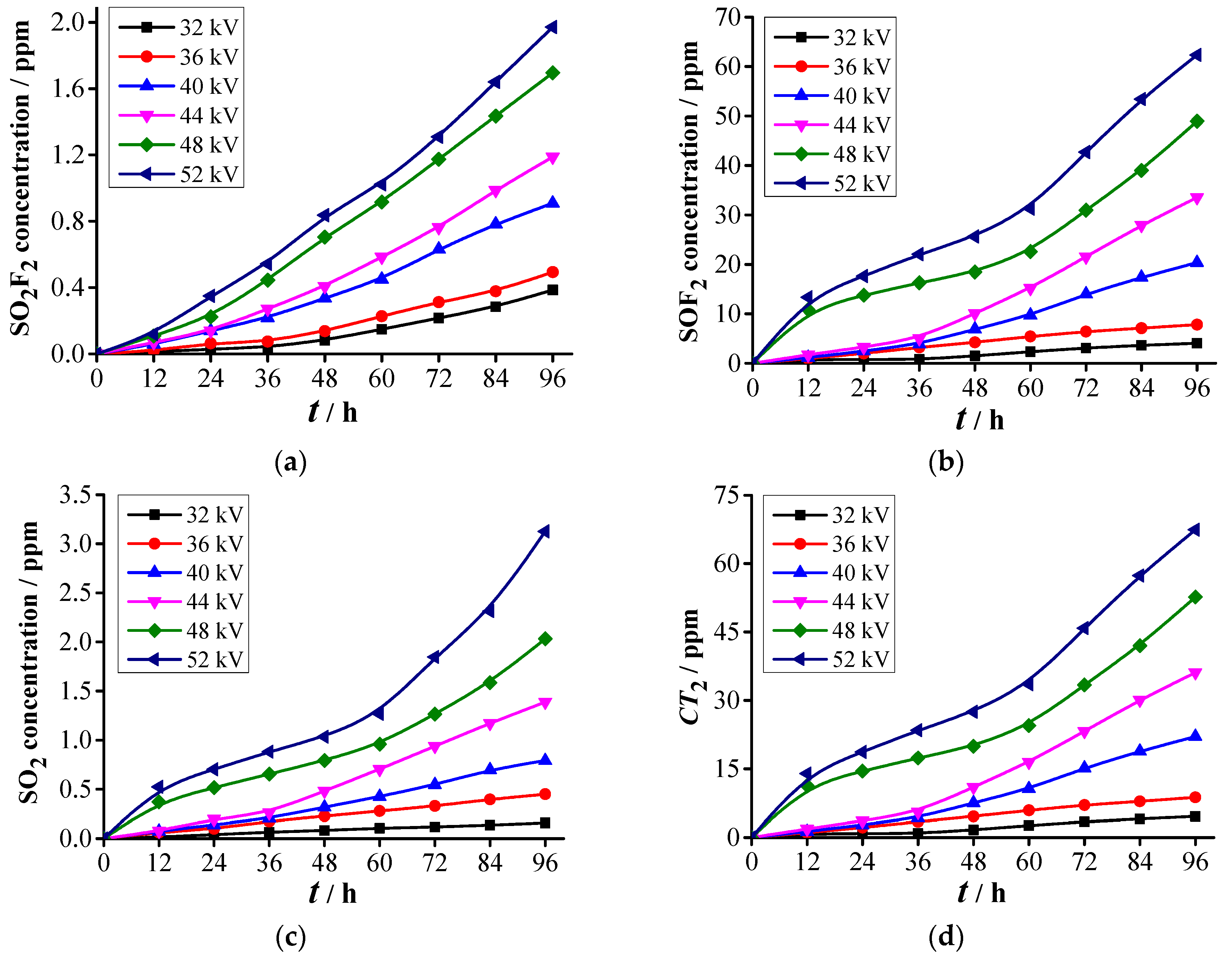
3.2.2. Formation Characteristics of Sulfur-Containing Components

SO₂F₂ is mainly produced through the reaction of SF₂ with O₂. The average O₂ concentration on the six experiments in the gas chamber is 1080 ppm. The sum of the concentration of the oxygen-containing components (CO₂, SO₂F₂, SOF₂, and SO₂) is less than 72 ppm, which indicates that O₂ is abundant in the formation of SO₂F₂. Thus, the formation characteristic of SO₂F₂ is mainly determined by the SF₂ concentration produced. Under the effect of the electric field, the charged particles hit the SF₆ molecules and break four S-F bonds to generate SF₂, which requires high-energy collision ionization [26,51]. The energy of the charged particle is not high when the voltage U ≤ 48 kV (Figure 9a). Therefore, the amount of the produced SF₂ is small, and the SO₂F₂ concentration grows slowly within 24 h. However, the SF₂ formed continues to accumulate with time, and the SO₂F₂ concentration presents an approximately linear growth trend after 36 h. When the voltage increases to 52 kV, the SO₂F₂ concentration shows an approximately linear increase with time. However, when the experimental voltage U ≤ 52 kV, with increasing voltage, the SO₂F₂ concentration remains less than 2 ppm, which illustrates that the SF₂ generated under the PD initiated by the particle defect can only produce a small amount of SO₂F₂.

SOF₂ is mainly generated through the reaction of SF₄ with H₂O. In the early stage of the experiment (t ≤ 36 h), when the voltage U ≤ 44 kV, the formation of SF₄ is limited by the PD energy to some extent, thus the SOF₂ concentration increases slowly (Figure 9b). When the voltage U > 44 kV, the increase rate of SOF₂ concentration accelerates, however, the increase rate within 12 h < t ≤ 36 h is lower than that within t ≤ 12 h. Which can be explained by two points: (1) with the increase in the applied voltage, the collision ionizations intensify, thus the SF₄ concentration grows rapidly; (2) the H₂O near the PD area are gradually consumed with time, which inhibits the formation of SOF₂ when 12 h < t ≤ 36 h. In the late stage of the experiment (t ≥ 60 h), the SF₄ produced continues to accumulate, gradually spreads into the main gas chamber area, and reacts with the H₂O in this area. The average H₂O concentration of six experiments in the gas chamber is 313 ppm. The highest concentration of SOF₂ in Figure 9b is 62.3 ppm. The H₂O concentration is five times higher than the SOF₂ concentration, which can satisfy the requirement for generating SOF₂. Therefore, the growth rate of SOF₂ concentration accelerates, and the SOF₂ concentration shows an approximately linear increase with time.

As shown in Figure 9c, the growth trend of SO₂ concentration with time is similar to that of SOF₂ concentration under the same voltage. SOF₂ reacts with H₂O to generate SO₂ and HF. The SO₂ concentration at 96 h is 2.03 ppm under 52 kV, which is much lower than the H₂O concentration (313 ppm) in the gas chamber. Therefore, the formation characteristic of SO₂ is mainly determined by the produced SOF₂, as in, the growth trend of SO₂ concentration is similar to that of SOF₂ concentration.

The concentration of (SO₂F₂ + SOF₂ + SO₂) can roughly reflect the amount of SF₆ gas decomposed by the PD. Therefore, CT₂ is defined to characterize the deterioration degree of SF₆ gas-insulated medium in DC-GIE, and its formula is as follows:

$$C{T}_2=C(\mathrm{S}{\mathrm{O}}_2{\mathrm{F}}_2)+C(\mathrm{S}\mathrm{O}{\mathrm{F}}_2)+C(\mathrm{S}{\mathrm{O}}_2)$$

(3)

where C(SO₂F₂), C(SOF₂), and C(SO₂) represent the concentrations of SO₂F₂, SOF₂, and SO₂ (unit: ppm), respectively. As shown in Figure 9, the growth trend of CT₂ with time is similar to that of SOF₂ concentration under the same voltage. When the voltage applied is 52 kV, the SOF₂ concentration is nearly 30 times the SO₂F₂ concentration and 20 times the SO₂ concentration at 96 h. Thus, the change trend of CT₂ is mainly determined by the SOF₂ produced. The change curves of CT₂ are different under three different PD levels. Thus, CT₂ can be associated with the PD severity.

4. PD Severity Diagnosis

The concentration ratios of SF₆ decomposed components for the PD recognition in GIE are proposed according to the three-ratio method used in oil chromatographic analysis to eliminate the influence of the volume effect and time effect on the fault diagnosis [22,23,24]. These concentration ratios have definite physical meaning but are not necessarily the optimal feature subset for PD recognition. These ratios do not necessarily have the maximum relevance with the PD types and are possibly relevant with each other, which will introduce redundant information to the PD recognition. And the other concentration ratios might be advantageous for PD recognition. Furthermore, the features applicable to the PD type recognition are not necessarily suitable for the PD severity diagnosis. Therefore, this study selects the optimal feature subset for PD severity diagnosis based on the minimum-redundancy-maximum-relevance (mRMR) principle.

4.1. mRMR Principle

mRMR is a feature selection method based on the mutual information. In this method, the features are selected according to the maximum statistical dependency principle [28,29,30,31,32,33]; it finds m features as the optimal subset with the maximum relevance to the target category and minimum redundancy between each other from all features. Maximum relevance (max D) and minimum redundancy (min R) are defined as follows:

$$\max D(S,c),D=\frac{1}{\left|S\right|}{\displaystyle \sum _{x_i\in S}I(x_i;c)}$$

(4)

$$\min R(S),R=\frac{1}{{\left|S\right|}^2}{\displaystyle \sum _{x_i,x_j\in S}I(x_i;x_j)}$$

(5)

where S is the selected feature subset; |S| is the number of features in S; I(x_i; c) is the mutual information between the feature x_i and the category c; and I(x_i; x_j) is the mutual information between the features x_i and x_j. Given two random continuous variables x and y, if their probability densities are p(x) and p(y), respectively, and their joint probability density is p(x, y), then the mutual information between x and y is defined as follows:

$$I(x;y)={\displaystyle \iint p(x,y)}\log \frac{p(x,y)}{p(x)p(y)}\mathrm{d}x\mathrm{d}y$$

(6)

When x and y are random discrete variables, Equation (6) can be written as follows:

$$I(x;y)={\displaystyle \sum _x{\displaystyle \sum _{y}p(x,y)\log \frac{p(x,y)}{p(x)p(y)}}}$$

(7)

In summary, the mRMR-based feature selection algorithm has two principles: (1) the MID principle, which requires the largest value of D (the mutual information between the feature and the category) minus R (the mutual information between the features) as shown in Equation (8); and (2) the MIQ principle, which requires the largest value of D divided by R as shown in Equation (9).

$$\max {\Phi }_1(D,R),{\Phi }_1=D-R$$

(8)

$$\max {\Phi }_2(D,R),{\Phi }_2=D/R$$

(9)

The set of all features (the number is n) is assumed as S_n, and m features (m < n) are selected from S_n according to the mRMR principle, which form the subset of S_m. The set of the remaining features is {S_n – S_m}. In order to obtain the subset S_m+1, another feature must be selected from {S_n – S_m} and combined with S_m to form S_m+1, which also meets mRMR principle. Therefore, the (m + 1)-th feature should satisfy Equation (10) or (11).

$$\underset{x_i\in \{S_n-S_m\}}{\max }[I(x_i;c)-\frac{1}{m}{\displaystyle \sum _{x_j\in S_m}I(x_i;x_j)}]$$

(10)

$$\underset{x_i\in \{S_n-S_m\}}{\max }[mI(x_i;c)/{\displaystyle \sum _{x_j\in S_m}I(x_i;x_j)}]$$

(11)

4.2. Feature Selection

The previous analysis showed close relationships between C(CF₄), C(CO₂), C(SO₂F₂), C(SOF₂), C(SO₂), CT₁, CT₂, and PD severity. Therefore, the set of concentration ratios for the PD severity diagnosis is constructed and shown in

Table 3. Concentration ratios for PD severity diagnosis and their corresponding labels.

Concentration Ratio	Label	Concentration Ratio	Label	Concentration Ratio	Label
C(CF4)/C(CO2)	1	C(CO2)/C(SOF2)	8	C(SO2F2)/CT2	15
C(CF4)/C(SO2F2)	2	C(CO2)/C(SO2)	9	C(SOF2)/C(SO2)	16
C(CF4)/C(SOF2)	3	C(CO2)/CT1	10	C(SOF2)/CT1	17
C(CF4)/C(SO2)	4	C(CO2)/CT2	11	C(SOF2)/CT2	18
C(CF4)/CT1	5	C(SO2F2)/C(SOF2)	12	C(SO2)/CT1	19
C(CF4)/CT2	6	C(SO2F2)/C(SO2)	13	C(SO2)/CT2	20
C(CO2)/C(SO2F2)	7	C(SO2F2)/CT1	14	CT1/CT2	21

, which also provides a corresponding label for each ratio to facilitate the subsequent analysis. The concentration ratios of SF₆ decomposed components are continuous variables. The probability density functions of these ratios must have been established to calculate the mutual information between the concentration ratios. However, no institution has conducted relevant statistical studies. Therefore, this study discretizes the concentration ratios [52].

x and y are assumed to be two concentration ratio vectors, and the number of the elements in x and y are both N. First, the elements in x are sorted in ascending order by value, and the value range of the elements in x is [x_min, x_max]. This range is subsequently divided into N_x subintervals on average. If the number of the elements in the i-th subinterval is n_x(i), the probability of the elements in x falling within the i-th subinterval is n_x(i)/N. Similarly, the probability of the elements in y falling within the j-th subinterval is n_y(j)/N, where n_y(j) is the number of the elements in y falling within the j-th subinterval. If the number of the elements in x falling within the i-th subinterval and the corresponding elements in y falling within the j-th subinterval is n_xy(i, j), then the probability of that is n_xy(i, j)/N. Therefore, the mutual information between x and y can be written as follows:

$$I(x;y)={\displaystyle \sum _{i=1}^{N_x}{\displaystyle \sum _{j=1}^{N_y}\frac{n_{xy}(i,j)}{N}\log \frac{N{n}_{xy}(i,j)}{n_x(i)n_y(j)}}}$$

(12)

where N_y is the number of the subintervals of vector y. If the value of n_x(i), n_y(j), or n_xy(i, j) is zero, then the value of $\log \frac{N{n}_{xy}(i,j)}{n_x(i)n_y(j)}$ is also denoted as zero.

If the concentration ratios of SF₆ decomposed components will be used to diagnose the PD severity in DC-GIE, then the influence of PD time on these ratios must be small. Even if insulation defects are found in DC-GIE, the concentrations of decomposed components are basically stabilized after a long run. Thus, the concentration ratios are unlikely to include large fluctuations with time. Similar to the first two ratios in Table 3, almost all of the 21 ratios in the table stabilize after 60 h (Figure 10). Therefore, the data of concentration ratios after 60 h are used to diagnose the PD severity.

The feature sorting of the concentrations and concentration ratios of SF₆ decomposed components for the PD severity diagnosis is conducted based on the principles of MID and MIQ, respectively. The feature order is shown in

Table 4. Feature order based on mRMR principle.

Feature Order	mRMR Principle
	MID	MIQ
Concentration order	CF4, SOF2, CO2, SO2, CT2, SO2F2, CT1	CF4, SOF2, SO2, CT2, CT1, SO2F2, CO2
Concentration ratio order	10, 4, 8, 1, 12, 5, 14, 2, 9, 3, 18, 7, 6, 11, 15, 16, 19, 21, 17, 20, 13	10, 4, 8, 1, 5, 12, 2, 3, 18, 14, 9, 6, 7, 11, 17, 15, 19, 21, 20, 16, 13

, and the concentration ratios in the table are indicated by their corresponding labels. The first two features, namely, CF₄ and SOF₂, of the concentrations are the same, and the first four features, namely, C(CO₂)/CT₁, C(CF₄)/C(SO₂), C(CO₂)/C(SOF₂), and C(CF₄)/C(CO₂), of the concentration ratios are also the same.

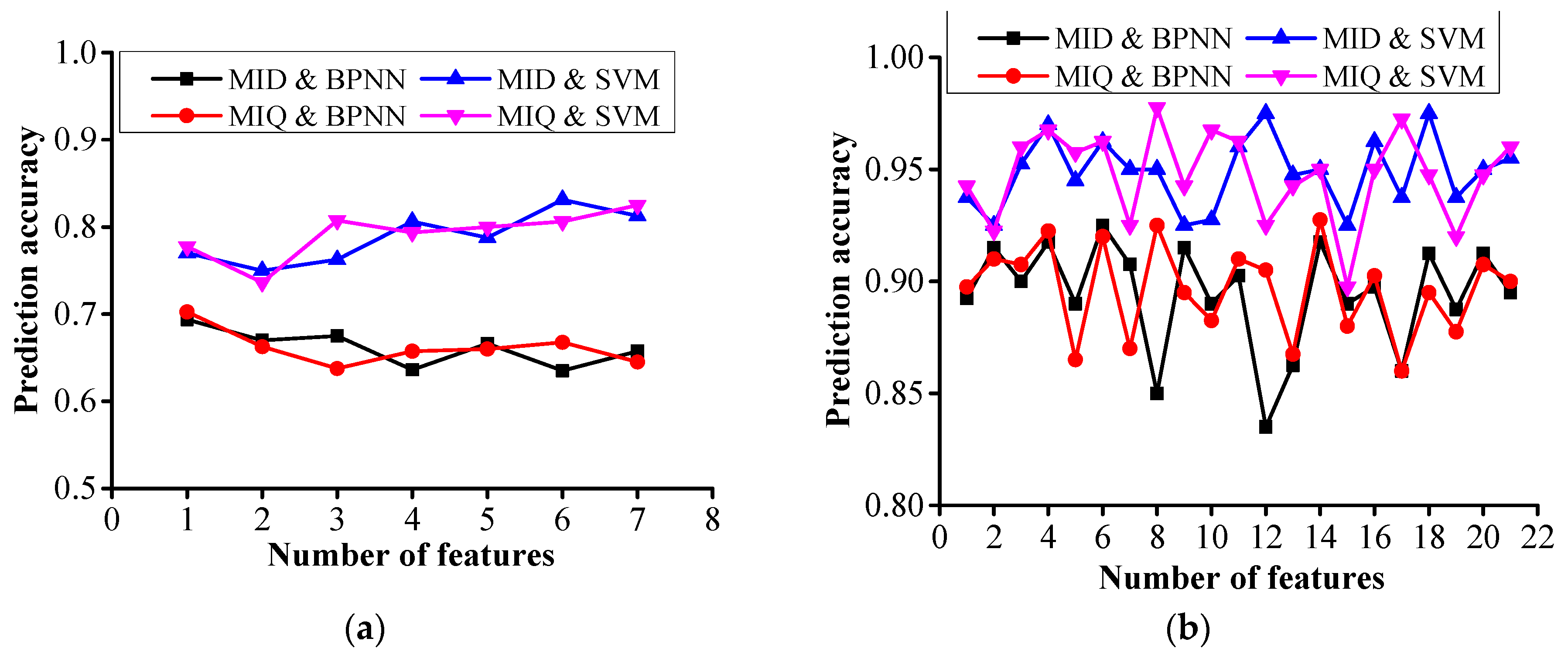
4.3. PD Severity Diagnosis

The back propagation neural network (BPNN) [24,34,35,36,37,38,39,40,41] and support vector machine (SVM) [41,42,43,44,45,46,47] algorithms are used to diagnose the PD severity. The concentrations and concentration ratios of SF₆ decomposed components are selected as the input data, and three PD levels (mild PD, medium PD, and dangerous PD) are the output results. The total samples are randomly divided into six equal parts, five of which are used as the training samples, and the remaining one is used as the test sample. The diagnosis results are shown in Figure 11, and the prediction accuracy is the average value of 100 diagnoses. The prediction accuracy of PD severity obtained by using the concentration ratios is higher than that obtained by using the concentrations, and the prediction accuracy obtained by using SVM is higher than that obtained by using BPNN. Therefore, the concentration ratios are more suitable than the concentrations as the feature quantities for PD severity diagnosis. The SVM algorithm is complex; when the number of features is large, the computational complexity is huge. When the concentration ratios are used to diagnose the PD severity, the prediction accuracy obtained by using BPNN is also high, and the computational complexity of which is moderate. Therefore, we can select a suitable algorithm to diagnose the PD severity according to the actual situation.

From the previous analysis, the first four concentration ratios, namely, C(CO₂)/CT₁, C(CF₄)/C(SO₂), C(CO₂)/C(SOF₂), and C(CF₄)/C(CO₂), obtained by using the MID- and MIQ-based feature selection algorithms, are the same.

Table 5. The highest three prediction accuracies and their corresponding concentration ratios.

mRMR Principle	Algorithm	Accuracy Order	Accuracy	Number of Features	Concentration Ratio Labels
MID	BPNN	1	92.5%	6	10, 4, 8, 1, 12, 5
		2	91.75%	4/14	10, 4, 8, 1/10, 4, 8, 1, 12, 5, 14, 2, 9, 3, 18, 7, 6, 11
		3	-	-	-
	SVM	1	97%	12/18	10, 4, 8, 1, 12, 5, 14, 2, 9, 3, 18, 7/10, 4, 8, 1, 12, 5, 14, 2, 9, 3, 18, 7, 6, 11, 15, 16, 19, 21
		2	-	-	-
		3	97.5%	4	10, 4, 8, 1
MIQ	BPNN	1	92.75%	14	10, 4, 8, 1, 5, 12, 2, 3, 18, 14, 9, 6, 7, 11
		2	92.5%	8	10, 4, 8, 1, 5, 12, 2, 3
		3	92.25%	4	10, 4, 8, 1
	SVM	1	97.75%	8	10, 4, 8, 1, 5, 12, 2, 3
		2	97.25%	17	10, 4, 8, 1, 5, 12, 2, 3, 18, 14, 9, 6, 7, 11, 17, 15, 19
		3	96.75%	4/10	10, 4, 8, 1/10, 4, 8, 1, 5, 12, 2, 3, 18, 14

shows the highest three prediction accuracies and their corresponding numbers of features of each curve in Figure 11b. When using these four concentration ratios to diagnose the PD severity, the prediction accuracy obtained is on the top three, and the difference from the highest accuracy does not exceed 1%. Therefore, this research recommends using C(CO₂)/CT₁, C(CF₄)/C(SO₂), C(CO₂)/C(SOF₂), and C(CF₄)/C(CO₂) to diagnose the PD severity initiated by a free metal particle defect in DC-GIE.

Twenty-four groups of concentration ratios in this paper are used as the training samples, and another set of experimental data is used as the test sample to verify the diagnosis performance of PD severity by using the abovementioned four concentration ratios. The concentration ratios in the test sample are obtained under the same experimental conditions as in this paper, and the deviations of the concentrations of SF₆ decomposed components between these two experiments are less than 10%. BPNN and SVM algorithms are used to diagnose the PD severity, and the confusion matrices of the diagnosis results are shown in

Table 6. Confusion matrix of the diagnosis result based on the back propagation neural network (BPNN).

Real PD Severity	Number of Samples in Each PD Level in the Diagnosis Result
	Mild PD	Medium PD	Dangerous PD
Mild PD	7	1	0
Medium PD	0	7	1
Dangerous PD	0	0	8

and

Table 7. Confusion matrix of the diagnosis result based on the support vector machine (SVM).

Real PD Severity	Number of Samples in Each PD Level in the Diagnosis Result
	Mild PD	Medium PD	Dangerous PD
Mild PD	8	0	0
Medium PD	0	7	1
Dangerous PD	0	0	8

. The prediction accuracy of PD severity by using BPNN algorithm is: (7 + 7 + 8)/24 = 91.67%, and that obtained by using SVM algorithm is: (8 + 7 + 8)/24 = 95.83%, which both obtain good diagnosis effects.

5. Discussion

The decomposition characteristics of SF₆ under different negative DC voltages are studied. The mRMR principle is used for the feature selection for PD severity diagnosis, and the BPNN and SVM algorithms are used to diagnose the PD severity. This research lays the foundation for the use of DCA method to diagnose the insulation faults in DC-GIE and to assess its insulation status. However, due to the limitations of the experimental conditions, only two kinds of voltage in each PD level are selected for the decomposition experiment of SF₆. More experiments should be performed in the future. H₂O, O₂, absorbent, and gas pressure in DC-GIE will affect the decomposition characteristics of SF₆; however, these factors are not considered in this study and thus require further research. In addition, more field data of SF₆ decomposed components should be obtained to verify and improve the performance of the proposed method in diagnosing PD severity.

6. Conclusions

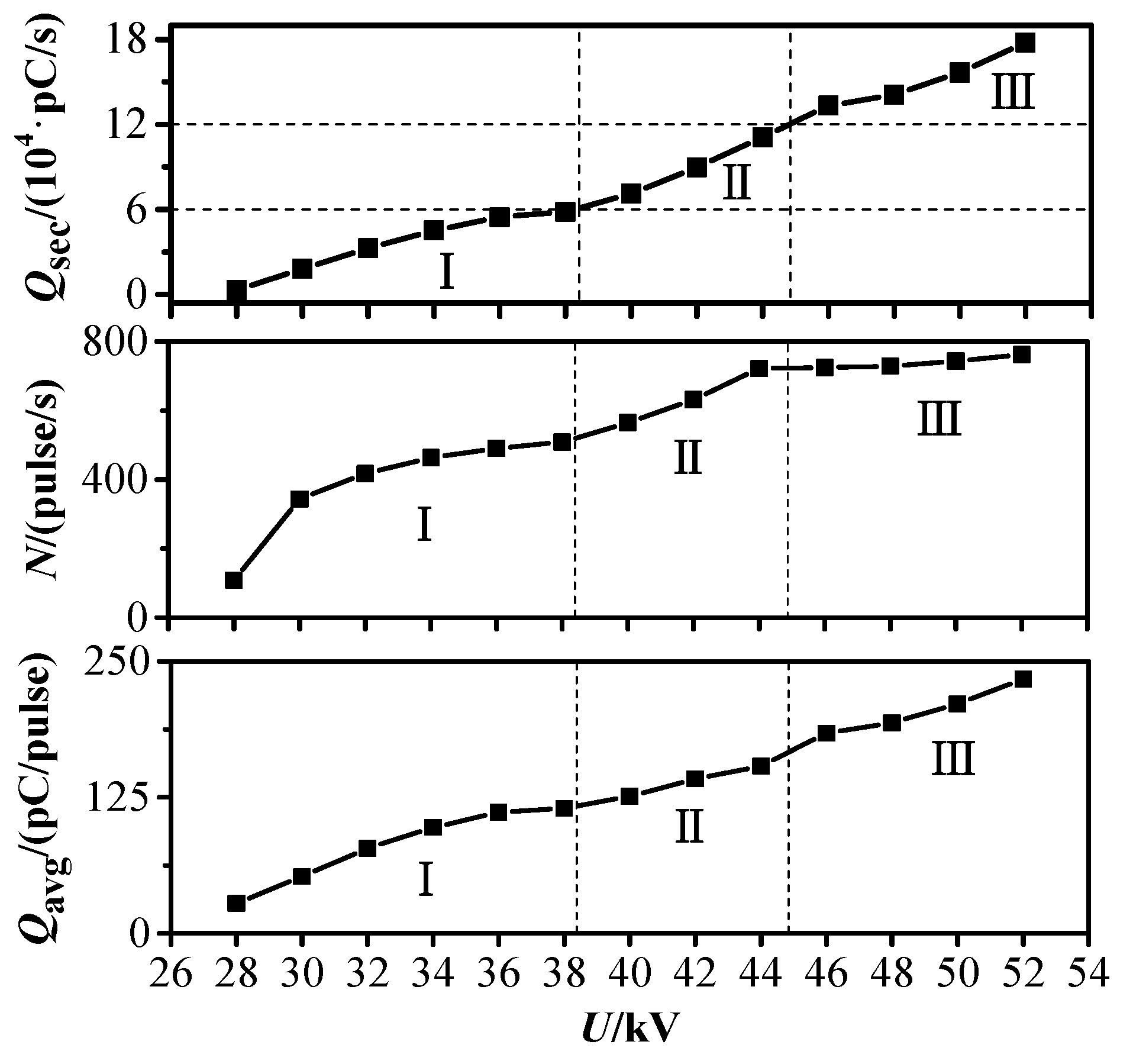
• The PD characteristics of the whole process from the initial PD to the breakdown initiated by free metal particle defect in DC-GIE are studied. The average discharge magnitude in a second Q_sec is proposed to be used to characterize the PD severity. Based on Q_sec, the PD is divided into three levels: mild PD, medium PD, and dangerous PD.
• Two kinds of voltage in each abovementioned PD level are selected for the decomposition experiment of SF₆. Experimental results show that five stable decomposed components, namely, CF₄, CO₂, SO₂F₂, SOF₂, and SO₂, are detected under each voltage. The PD severity has close relationships with C(CF₄), C(CO₂), C(SO₂F₂), C(SOF₂), C(SO₂), CT₁, and CT₂. The concentrations and concentration ratios of SF₆ decomposed components can be used to diagnose the PD severity.
• mRMR-based feature selection algorithm is used to sort the concentrations and concentration ratios of SF₆ decomposed components, and BPNN and SVM algorithms are used to diagnose the PD severity. The prediction accuracy of PD severity obtained by using the concentration ratios is higher than that obtained by using the concentrations, and the use of C(CO₂)/CT₁, C(CF₄)/C(SO₂), C(CO₂)/C(SOF₂), and C(CF₄)/C(CO₂) shows good performance in diagnosing the PD severity.

References

1. Benato, R.; Dughiero, F.; Forzan, M.; Paolucci, A. Proximity effect and magnetic field calculation in GIL and in isolated phase bus ducts. IEEE Trans. Magn. 2002, 38, 781–784. [Google Scholar] [CrossRef]
2. Benato, R.; Mario, C.D.; Koch, H. High-capability applications of long gas-insulated lines in structures. IEEE Trans. Power Del. 2007, 22, 619–626. [Google Scholar] [CrossRef]
3. Benato, R.; Brunello, P.; Fellin, L. Thermal behavior of EHV gas-insulated lines in Brenner pass pilot tunnel. IEEE Trans. Power Del. 2010, 25, 2717–2725. [Google Scholar] [CrossRef]
4. Benato, R.; Dughiero, F. Solution of coupled electromagnetic and thermal problems in gas-insulated transmission lines. IEEE Trans. Magn. 2003, 39, 1741–1744. [Google Scholar] [CrossRef]
5. Benato, R.; Napolitano, D. Reliability assessment of EHV gas-insulated transmission lines: Effect of redundancies. IEEE Trans. Power Del. 2008, 23, 2174–2181. [Google Scholar] [CrossRef]
6. Tenzer, M.; Koch, H.; Imamovic, D. Underground transmission lines for high power AC and DC transmission. In Proceedings of the 2016 IEEE/PES Transmission and Distribution Conference and Exposition, Dallas, TX, USA, 3–5 May 2016. [Google Scholar]
7. Magier, T.; Tenzer, M.; Koch, H. Direct current gas-insulated transmission lines. IEEE Trans. Power Del. 2017. [Google Scholar] [CrossRef]
8. Mendik, M.; Lowder, S.M.; Elliott, F. Long term performance verification of high voltage DC GIS. In Proceedings of the 1999 IEEE Transmission and Distribution Conference, New Orleans, LA, USA, 11–16 April 1999; pp. 484–488. [Google Scholar]
9. Ohki, Y. Thyristor valves and GIS in Kii channel HVDC link. IEEE Electr. Insul. Mag. 2001, 17, 78–79. [Google Scholar] [CrossRef]
10. Hasegawa, T.; Yamaji, K.; Hatano, M. Development of insulation structure and enhancement of insulation reliability of 500 kV DC GIS. IEEE Trans. Power Del. 1997, 12, 192–202. [Google Scholar] [CrossRef]
11. Hasegawa, T.; Yamaji, K.; Hatano, M. DC dielectric characteristics and conception of insulation design for DC GIS. IEEE Trans. Power Del. 1996, 11, 1776–1782. [Google Scholar] [CrossRef]
12. Beyer, C.; Jenett, H.; Kfockow, D. Influence of reactive SFx gases on electrode surfaces after electrical discharges under SF6 atmosphere. IEEE Trans. Dielectr. Electr. Insul. 2000, 7, 234–240. [Google Scholar] [CrossRef]
13. Chu, F.Y. SF6 decomposition in gas-insulated equipment. IEEE Trans. Dielectr. Electr. Insul. 1986, 21, 693–725. [Google Scholar] [CrossRef]
14. Van Brunt, R.J.; Herron, J.T. Fundamental processes of SF6 decomposition and oxidation in glow and corona discharges. IEEE Trans. Dielectr. Electr. Insul. 1990, 25, 75–94. [Google Scholar] [CrossRef]
15. Chang, C.; Chang, C.S.; Jin, J.; Hoshino, T.; Hanai, M.; Kobayashi, N. Source classification of partial discharge for gas insulated substation using wave shape pattern recognition. IEEE Trans. Dielectr. Electr. Insul. 2005, 12, 374–386. [Google Scholar] [CrossRef]
16. Dreisbusch, K.; Kranz, H.G.; Schnettler, A. Determination of a failure probability prognosis based on PD-diagnostics in GIS. IEEE Trans. Dielectr. Electr. Insul. 2008, 15, 1707–1714. [Google Scholar] [CrossRef]
17. Istad, M.; Runde, M. Thirty-six years of service experience with a national population of gas-insulated substations. IEEE Trans. Power Del. 2010, 25, 2448–2454. [Google Scholar] [CrossRef]
18. Van Brunt, R.J. Production rates for oxy-fluorides SOF2, SO2F2 and SOF4 in SF6 corona discharges. J. Res. Natl. Bur. Stand. 1985, 90, 229–253. [Google Scholar] [CrossRef]
19. Piemontesi, M.; Niemeyer, L. Sorption of SF6 and SF6 decomposition products by activated alumina and molecular sieve 13X. In Proceedings of the 1996 IEEE International Symposium on Electrical Insulation, Montreal, QC, Canada, 16–19 June 1996; pp. 828–838. [Google Scholar]
20. Van Brunt, R.J.; Herron, J.T. Plasma chemical model for decomposition of SF6 in a negative glow corona discharge. Phys. Scr. 1994, 53, 9–29. [Google Scholar] [CrossRef]
21. Prakash, K.S.; Srivastava, K.D.; Morcos, M.M. Movement of particles in compressed SF6 GIS with dielectric coated enclosure. IEEE Trans. Dielectr. Electr. Insul. 1997, 4, 344–347. [Google Scholar] [CrossRef]
22. Tang, J.; Liu, F.; Zhang, X.X.; Meng, Q.H.; Zhou, J.B. Partial discharge recognition through an analysis of SF6 decomposition products part 1: Decomposition characteristics of SF6 under four different partial discharges. IEEE Trans. Dielectr. Electr. Insul. 2012, 19, 29–36. [Google Scholar] [CrossRef]
23. Tang, J.; Liu, F.; Meng, Q.H.; Zhang, X.X.; Tao, J.G. Partial discharge recognition through an analysis of SF6 decomposition products part 2: Feature extraction and decision tree-based pattern recognition. IEEE Trans. Dielectr. Electr. Insul. 2012, 19, 37–44. [Google Scholar] [CrossRef]
24. Tang, J.; Yang, X.; Ye, G.X.; Yao, Q.; Miao, Y.L.; Zeng, F.P. Decomposition characteristics of SF6 and partial discharge recognition under negative DC conditions. Energies 2017, 10, 556. [Google Scholar] [CrossRef]
25. Majidi, M.; Oskuoee, M. Improving pattern recognition accuracy of partial discharges by new data preprocessing methods. Electr. Power Syst. Res. 2015, 119, 100–110. [Google Scholar] [CrossRef]
26. Tang, J.; Zeng, F.P.; Pan, J.Y.; Zhang, X.X.; Yao, Q. Correlation analysis between formation process of SF6 decomposed components and partial discharge qualities. IEEE Trans. Dielectr. Electr. Insul. 2013, 20, 864–875. [Google Scholar] [CrossRef]
27. Tang, J.; Pan, J.Y.; Zhang, X.X.; Zeng, F.P.; Yao, Q.; Hou, X.Z. Correlation analysis between SF6 decomposed components and charge magnitude of partial discharges initiated by free metal particles. IET Sci. Meas. Technol. 2014, 8, 170–177. [Google Scholar] [CrossRef]
28. Ashkezari, A.D.; Ma, H.; Saha, T.K.; Cui, Y. Investigation of feature selection techniques for improving efficiency of power transformer condition assessment. IEEE Trans. Dielectr. Electr. Insul. 2014, 21, 836–844. [Google Scholar] [CrossRef]
29. Peng, H.C.; Long, F.H.; Ding, C. Feature selection based on mutual information: Criteria of max-dependency, max-relevance, and min-redundancy. IEEE Trans. Pattern Anal. Mach. Intell. 2005, 27, 1226–1238. [Google Scholar] [CrossRef] [PubMed]
30. Li, Y.B.; Yang, Y.T.; Li, G.Y. A fault diagnosis scheme for planetary gearboxes using modified multi-scale symbolic dynamic entropy and mRMR feature selection. Mech. Syst. Signal. Pr. 2017, 91, 295–312. [Google Scholar] [CrossRef]
31. Escalona-Vargas, D.; Siegel, E.R.; Murphy, P.; Lowery, C.L.; Eswaran, H. Selection of reference channels based on mutual information for frequency-dependent subtraction method applied to fetal biomagnetic signals. IEEE Trans. Biomed. Eng. 2017, 64, 1115–1122. [Google Scholar] [CrossRef] [PubMed]
32. Xu, Y.; Ding, Y.X.; Ding, J.; Wu, L.Y.; Xue, Y. Mal-Lys: Prediction of lysine malonylation sites in proteins integrated sequence-based features with mRMR feature selection. Sci. Rep. 2016, 6, 38318. [Google Scholar] [CrossRef] [PubMed]
33. Ramirez-Gallego, S.; Lastra, I.; Martinez-Rego, D.; Bolon-Canedo, V.; Benitez, J.M.; Herrera, F.; Alonso-Betanzos, A. Fast-mRMR: Fast minimum redundancy maximum relevance algorithm for high-dimensional big data. Int. J. Intell. Syst. 2017, 32, 134–152. [Google Scholar] [CrossRef]
34. Aminian, M.; Aminian, F. Neural-network based analog-circuit fault diagnosis using wavelet transform as preprocessor. IEEE Trans. Circuits Syst. II Analog Digit. Signal Process. 2000, 47, 151–156. [Google Scholar] [CrossRef]
35. Karnin, E.D. A simple procedure for punning back-propagation trained neural networks. IEEE Trans. Neural Netw. 1990, 1, 239–242. [Google Scholar] [CrossRef] [PubMed]
36. Mas’ud, A.A.; Albarracín, R.; Ardila-Rey, J.A.; Muhammad-Sukki, F.; Illias, H.A.; Bani, N.A.; Munir, A.B. Artificial neural network application for partial discharge recognition: Survey and future directions. Energies 2016, 9, 574–591. [Google Scholar] [CrossRef]
37. Majidi, M.; Fadali, M.S.; Etezadi-Amoli, M.; Oskuoee, M. Partial discharge pattern recognition via sparse representation and ANN. IEEE Trans. Dielectr. Electr. Insul. 2015, 22, 1061–1070. [Google Scholar] [CrossRef]
38. Gulski, E.; Krivda, A. Neural networks as a tool for recognition of partial discharges. IEEE Trans. Dielectr. Electr. Insul. 1993, 28, 984–1001. [Google Scholar] [CrossRef]
39. Satish, L.; Zaengl, W.S. Artificial neural networks for recognition of 3-D partial discharge patterns. IEEE Trans. Dielectr. Electr. Insul. 1994, 1, 265–275. [Google Scholar] [CrossRef]
40. Hozumi, N.; Okamoto, T.; Imajo, T. Discrimination of partial discharge patterns using a neural network. IEEE Trans. Dielectr. Electr. Insul. 1992, 27, 550–556. [Google Scholar] [CrossRef]
41. Leng, X.Z.; Wang, J.H.; Ji, H.B.; Wang, Q.G.; Li, H.M.; Qian, X.; Li, F.Y.; Yang, M. Prediction of size-fractionated airborne particle-bound metals using MLR, BP-ANN and SVM analyses. Chemosphere 2017, 180, 513–522. [Google Scholar] [CrossRef] [PubMed]
42. Tang, J.; Zhuo, R.; Wang, D.B.; Wu, J.R.; Zhang, X.X. Application of SA-SVM incremental algorithm in GIS PD pattern recognition. J. Electr. Eng. Technol. 2016, 11, 192–199. [Google Scholar] [CrossRef]
43. Tang, J.; Tao, J.G.; Zhang, X.X.; Liu, F. Multiple SVM-RFE for feature subset selection in partial discharge pattern recognition. Int. Rev. Electr. Eng. I. 2012, 7, 5240–5246. [Google Scholar]
44. Tang, J.; Wang, D.B.; Fan, L.; Zhuo, R.; Zhang, X.X. Feature parameters extraction of GIS partial discharge signal with multifractal detrended fluctuation analysis. IEEE Trans. Dielectr. Electr. Insul. 2015, 22, 3037–3045. [Google Scholar] [CrossRef]
45. Naseri, F.; Jafari, F.; Mohseni, E.; Tang, W.C.; Feizbakhsh, A.; Khatibinia, M. Experimental observations and SVM-based prediction of properties of polypropylene fibres reinforced self-compacting composites incorporating nano-CuO. Coustr. Build. Mater. 2017, 143, 589–598. [Google Scholar] [CrossRef]
46. Wei, Q.; Wu, B.; Xu, D.W.; Zargari, N.R. Natural sampling SVM-based common-mode voltage reduction in medium-voltage current source rectifier. IEEE Trans. Power Electr. 2017, 32, 7553–7560. [Google Scholar] [CrossRef]
47. Gonzalez-Costa, J.J.; Reigosa, M.J.; Matias, J.M.; Covelo, E.F. Soil Cd, Cr, Cu, Ni, Pb and Zn sorption and retention models using SVM: Variable selection and competitive model. Sci. Total Environ. 2017, 593, 508–522. [Google Scholar] [CrossRef] [PubMed]
48. IEC 60270:2000 High-voltage Test Techniques—Partial Discharge Measurements. Available online: http://www.doc88.com/p-868119919771.html (accessed on 20 June 2017).
49. DL/T 596–1996 Preventive Test Code for Electric Power Equipment. Available online: http://www.doc88.com/p-9763610841190.html (accessed on 20 June 2017).
50. Zhou, W.J.; Zheng, Y.; Yang, S.; Li, H.; Wang, B.S.; Qiao, S.Y. Detection of intense partial discharge of epoxy insulation in SF6 insulated equipment using carbonyl sulfide. IEEE Trans. Dielectr. Electr. Insul. 2016, 23, 2942–2948. [Google Scholar] [CrossRef]
51. Tang, J.; Zeng, F.P.; Zhang, X.X.; Pan, J.Y.; Yao, Q.; Hou, X.Z.; Tang, Y. Relationship between decomposition gas ratios and partial discharge energy in GIS, and the influence of residual water and oxygen. IEEE Trans. Dielectr. Electr. Insul. 2014, 21, 1226–1234. [Google Scholar] [CrossRef]
52. Kraskov, A.; Stögbauer, H.; Grassberger, P. Estimating mutual information. Phys. Rev. E Stat. Nonlin. Soft Matter Phys. 2004, 69, 066138. [Google Scholar] [CrossRef] [PubMed]
Figure 1. Experimental platform of SF6 decomposition under negative DC-partial discharge (PD).
Energies 10 01119 g001
Figure 2. Structure of PD gas chamber: 1: gas chamber; 2: High-voltage (HV) bushing; 3: HV conductor; 4: ball valve; 5: vacuum pressure gauge; 6: vacuum pump; 7: injection port; 8: support insulator; 9: ground conductor; 10: insulation defect; and 11: sampling port.
Energies 10 01119 g002
Figure 3. Calibration curve of PD magnitude.
Energies 10 01119 g003
Figure 4. Insulation defect model (Unit: mm).
Energies 10 01119 g004
Figure 5. Experimental voltage and duration.
Energies 10 01119 g005
Figure 6. Three PD parameters over the applied voltage.
Energies 10 01119 g006
Figure 7. Formation process of SF6 decomposed components.
Energies 10 01119 g007
Figure 8. Change of carbon-containing components with time: (a) CF4; (b) CO2; and (c) CT1.
Energies 10 01119 g008aEnergies 10 01119 g008b
Figure 9. Change of sulfur-containing components with time: (a) SO2F2; (b) SOF2; (c) SO2; and (d) CT2.
Energies 10 01119 g009
Figure 10. Change of concentration ratios with time: (a) C(CF4)/C(CO2); and (b) C(CF4)/C(SO2F2).
Energies 10 01119 g010
Figure 11. Predication accuracy over the number of features: (a) concentration feature; and (b) concentration ratio feature.
Energies 10 01119 g011