
Demand Side Management in Nearly Zero Energy Buildings Using Heuristic Optimizations
by
 , , , and
Nadeem Javaid
1,* ,
,
Sardar Mehboob Hussain
1,
Ibrar Ullah
2,3,
Muhammad Asim Noor
1,
Wadood Abdul
4,
Ahmad Almogren
4 and
Atif Alamri
4 1
Department of Computer Science, COMSATS Institute of Information Technology, Islamabad 44000, Pakistan
2
University of Engineering and Technology Peshawar, Bannu 28100, Pakistan
3
Capital University of Science and Technology, Islamabad 44000, Pakistan
4
Research Chair of Pervasive and Mobile Computing, College of Computer and Information Sciences, King Saud University, Riyadh 11633, Saudi Arabia
*
Author to whom correspondence should be addressed.
Energies 2017, 10(8), 1131; https://doi.org/10.3390/en10081131
Submission received: 29 June 2017
/
Revised: 25 July 2017
/
Accepted: 29 July 2017
/
Published: 2 August 2017
(This article belongs to the Special Issue Battery Energy Storage Applications in Smart Grid)
Abstract
:Today’s buildings are responsible for about 40% of total energy consumption and 30–40% of carbon emissions, which are key concerns for the sustainable development of any society. The excessive usage of grid energy raises sustainability issues in the face of global changes, such as climate change, population, economic growths, etc. Traditionally, the power systems that deliver this commodity are fuel operated and lead towards high carbon emissions and global warming. To overcome these issues, the recent concept of the nearly zero energy building (nZEB) has attracted numerous researchers and industry for the construction and management of the new generation buildings. In this regard, this paper proposes various demand side management (DSM) programs using the genetic algorithm (GA), teaching learning-based optimization (TLBO), the enhanced differential evolution (EDE) algorithm and the proposed enhanced differential teaching learning algorithm (EDTLA) to manage energy and comfort, while taking the human preferences into consideration. Power consumption patterns of shiftable home appliances are modified in response to the real-time price signal in order to get monetary benefits. To further improve the cost and user discomfort objectives along with reduced carbon emission, renewable energy sources (RESs) are also integrated into the microgrid (MG). The proposed model is implemented in a smart residential complex of multiple homes under a real-time pricing environment. We figure out two feasible regions: one for electricity cost and the other for user discomfort. The proposed model aims to deal with the stochastic nature of RESs while introducing the battery storage system (BSS). The main objectives of this paper include: (1) integration of RESs; (2) minimization of the electricity bill (cost) and discomfort; and (3) minimizing the peak to average ratio (PAR) and carbon emission. Additionally, we also analyze the tradeoff between two conflicting objectives, like electricity cost and user discomfort. Simulation results validate both the implemented and proposed techniques.
1. Introduction
According to the European commission’s report [1], buildings consume about 40% of overall energy and are responsible for 30–40% of carbon emissions. As energy, water, land and other resources are required for the construction, maintenance, control and demolition of all buildings [2,3], so the carbon emissions and wastes due to building construction and maintenance cannot be neglected. Due to all of these reasons, scientist and researchers began to start using passive techniques for building construction and active techniques for control and management while taking into account human needs regarding comfort and green environment.
In addition, the European “Energy Performance of Buildings Directive (EPBD)” released in 2010 and “Energy Efficiency Directive (EED)” released in 2012 led the member countries of the European Union to readjust their legislation regarding building energy management for sustainable development of society. According to this, from the year 2019, all new buildings will be nearly zero energy buildings (nZEBs), and by the end of year 2020, all buildings will have to maintain nZEB [4,5]; where the term zero energy building (ZEB) is defined as: “an energy efficient buildings where annual energy delivered to home/residential sector is less than or equal to the total energy generation from on-side or standalone renewable energy sources (RESs)” [6]. However, the concept of ZEB can be characterized as: (i) grid-connected ZEB; and (ii) stand-alone or autonomous ZEBs. The stand-alone ZEBs are further separated into three categories [7]; Figure 1.
- nZEB: a ZEB connected to grid having a nearly zero energy balance. This means that the energy consumption in any building or sector is slightly greater than the total renewable energy.
- net zero energy building (NZEB): a ZEB connected to grid having zero energy balance. The total energy consumption and generation are almost equal.
- positive energy building (PEB): has a positive energy balance. The energy consumption in PEB is less than the energy generation from renewable sources where surplus energy is sold back to the grid.
In traditional energy generation systems, fossil fuels dominate as the power generation sources and are responsible for greenhouse gas (GHG) emissions. The challenge is not only to reduce GHG emissions, but also to increase electricity generation in view of socio-economic aspects of generation. RESs are considered as future replacement with zero carbon emission and low price electricity producers. RESs are intermittent, uncertain and random in nature; they do not produce a fixed amount of energy and are heavily dependent on weather, season and area. Integration of advanced information and communication technology (ICT) into the traditional power grid forms the smart grid (SG) [8].
An emerging type of distributed generation network called the microgrid (MG) is perceived as a medium voltage or low voltage power system with small distributed generation, few controllable distributed loads and on-site energy storage. One of the key underpinnings of MG, which allows it to dominate traditional grids, is the usage of RESs at the consumer level. Improvisation of the power grid has led to many challenges and issues, e.g., protection, selectivity, security, adaptability, scalability, reliability and many more [9]. Hybrid RESs with a battery storage system (BSS) are intensively discussed in the literature and, therefore, are widely accepted in order to cater to the uncertainty of RESs. Two major parties are involved in the operation of MG, i.e., consumers and the utility. Demand side management (DSM) offers demand response (DR) programs to the residential consumers in order to change daily electricity usage pattern in response to some incentives. These incentives are usually monetary rebates.
Major objectives of SG include reduced electricity bill, reduced peak to average ratio (PAR), maximized user comfort and balanced power consumption [10]. In [11], the authors use integer linear programming (ILP) to reduce the daily electricity bill of residential consumers. An approximate dynamic programming (DP) is used in [12] to reduce the electricity burden and PAR on the main power grid. An energy sale mechanism among different MGs is proposed using the game theoretic approach. A particle swarm optimization (PSO)-based DR program is discussed in [13] to curtail PAR and minimize daily consumption cost in the presence of RESs. In [14], two heuristic techniques, i.e., teaching learning-based optimization (TLBO) and the differential evolution (DE) algorithm are used to reduce cost and increase the comfort level of users.
In this paper, we design an energy management model (EMM) in nZEB using genetic algorithm (GA), TLBO, enhanced differential evolution (EDE) and our novel proposed EDTLA. Our main focus is RE integration and local distributed energy resources (DERs) scheduling in order to meet electricity and heat demands while reducing carbon emissions. We also compute the feasible regions for cost and user discomfort. A tradeoff between cost and comfort is also shown under the four different techniques. For this study, the time interval and time slot are used interchangeably. Similarly, electrical loads and electric tasks can be referred to as home appliances.
The remainder of the paper is organized as follows. Section 2 is comprised of recent related work. The problem description is provided in Section 3. Section 4 depicts the detailed description of the proposed model. The heuristic techniques are described in Section 5. The linear optimizations model is discussed in Section 6. Simulation findings and results are inscribed in Section 7. Lastly, in Section 8, concluding remarks are presented followed by the future work.
2. Related Work
In order to optimally schedule home tasks and DERs in residential MG, several methods have been proposed in the literatures [9,10,11,12,13,14,15,16,17,18,19,20,21,22,23,24,25,26,27,28,29,30]. Some of the recent approaches are discussed hereunder.
The analysis and sizing of RE in coordination with BSS is discussed in [15], and a hybrid model is proposed using mixed ILP (MILP). One year of available weather data is used to predict the weather profile of the next three years and then is used to figure out the optimal size of the wind turbine (WT), photovoltaic (PV) and thermal load profile for the residential building. The authors maximize the use of RE and reduce the burden of high power demand at the grid.
In [16], the authors present a complete nZEB framework and propose various methods regarding the implementation point of view. In another work [4], the authors implement an NZEB concept and propose a fuzzy logic-based energy management system for lighting, shading and HVAC systems. The authors implement various configurations, while taking into consideration walls, window geometry and glass properties. Regarding implementation, it was found that for a given amount of solar radiation, each room requires a diversified management system to maintain balance between comfort and energy management. A GUI-based energy and comfort management system for ZEB is proposed in [7]. A multiagent system is used to control distributed loads, while a particle swarm optimization algorithm is used to manage comfort and energy in the residential sector.
An active controller is proposed in [13] to optimally integrate the heating and cooling system in MG. The research improves the reliability of MG and minimizes the cost of MG, the size of RE resources and imported energy from the grid. The main purpose of this study is to minimize peak load and consumption cost.
In [17], the authors propose an SG equipped with 100% RESs to satisfy electricity and heating demands. BSS is used to deal with the fluctuating behavior of RESs. Combined heat and power (CHP) plants and district heating and cooling systems are introduced, which are responsible for providing heating and cooling loads to the households and other commercial buildings.
A cooperative interaction between the AD system (ADS) connected to multiple grids and the energy system is formulated in [18], and a dynamic energy management strategy is proposed. The first interaction is between MG and ADNs, whereas, the other is among different MGs. The authors propose a dynamic energy management technique for cooperation between MG and ADSs that caters to the influences of the high penetration of RESs. The work in [19] considered real-time energy storage management to increase the RE share in MG. The authors use an off-line algorithm for optimization and proposed a novel sliding window-based on-line algorithm. The main objectives of the research are to minimize the cost of power purchased from the grid and to maximize the penetration of RESs in MG. The cost function is formulated by the strictly convex function and solved using DP.
In [20], the joint operation of energy storage and load scheduling with RESs is considered in the residential domain. Electricity demand, starting times of appliances, the length of operation times of appliances and RE generation are considered as random and stochastic. The stochastic nature of the problem is solved by modifying the Lyapunov optimization technique. Regarding ZEB, an nZEB can be achieved by integrating RESs, such as solar and wind. In [21], the authors consider Vietnam, where solar energy is infrequently used in residential sectors. To promote energy management along with the integration of solar energy, a solar panel of 15-kW capacity is installed in the rooftop to compensate energy demand. However, prior to the installation of the solar panels, it is required to estimate the energy obtained from these panels. For this purpose, the PVSYST simulation tool has been used.
A home energy management system (HEMS) is proposed in [22,23], using different heuristic techniques. GA, BPSO and ACO are used to design a HEMS scheduler, which optimally schedules home appliances under large-scale penetration of RESs. The main objectives are to reduce the daily electricity bill and PAR.
In [11], an energy control system is proposed in a smart home of the residential domain. Different types of appliances are scheduled according to the given time frame. The optimization problem is solved using LP. The major objective is to reduce the electricity bill. A tradeoff between cost and discomfort is also analyzed using the Taguchi loss function.
Day-ahead scheduling of all resources for optimal operation of MG is proposed in [24]. The authors claim that one-day-ahead scheduling can avoid vulnerabilities and ensures the consistent operation of MG. An agent-based modeling (ABM) technique is used where each agent acts as a bus and provides information about losses and other attacks.
The participation of different DSM strategies in HEMS is analyzed in [25]. The major focus of this paper is to develop HEMS and DSM systems in order to reduce the electricity bill and maximize RE usage. The use of different incentive-based algorithmic techniques in DSM is analyzed, and their impact is elaborated.
The load scheduling and power trading problems in the residential area of MG with a large share of RE are discussed in [12]. An approximate DP is used for appliance scheduling, and a game theoretic approach is used for power trading among different users. All users, having excess generation, participate in a gamble, and the first winner is prioritized to sell excess generation first. In this way, every user reduces power usage and tries to sell maximum energy, which generates revenue and lowers the electricity bill.
In [26], electric vehicles (EVs) are integrated with MG in the presence of RESs. The major focus is to reduce power losses and improve the stability of MG under the large-scale integration of EVs. The DE algorithm is used to solve the multi-objective nature of the problem.
In [27], the authors use the real time pricing (RTP) signal in DSM programs to reduce the daily electricity bill and PAR. A new load scheduling learning (LSL) algorithm is proposed, which schedules appliances after learning from a series of actions. The change in load scheduling, power demand and pricing signal are modeled as a Markov decision process, and their information is stored with respect to each time slot.
An MG is formed with local DERs in which heat and electricity demand is provided to consumers in [28]. The former is provided by local generators like the CHP and boiler, whereas the latter is provided by WT, PV generation and energy import from the main grid. The authors aim at reducing the electricity expense and carbon emissions.
3. Problem Description
In SG, electricity bill minimization, power consumption minimization, PAR reduction, user comfort maximization and RESs integration are key challenges. Numerous mathematical and heuristic-based strategies have been proposed to deal with these optimization problems. Predominantly, user comfort is ignored to minimize the inevitably growing electricity bill problem. Existing DSM techniques target the electricity bill reduction while neglecting either PAR or the user comfort level. The randomness of the power usage pattern affects the optimal energy consumption schedule and user cost minimization at the consumer level. The authors in [28] proposed an MILP-based energy consumption model to reduce electricity consumption cost and GHG emissions. However, integration of RESs, PAR and user comfort are not tackled in the proposed model. However, Ref. [11] considered the electricity bill minimization along with user comfort maximization. The authors use ILP to solve the convex nature of the optimization problem, and a tradeoff between cost and discomfort is also computed. Although the scheduling strategy reduces the energy expense, RESs integration can further decrease the electricity bill, carbon emissions and PAR. Residential load scheduling and power trading among different homes in the presence of RESs is discussed in [12]. Stochastic optimization is used for the residential scheduling, whereas a game theoretic approach is adopted for power trading among multiple homes. PAR and user comfort level are not considered, which are crucial parameters of SG. No proper mechanism is provided for power flow from one user to another. A GA-based DR program for HEMS is proposed in [31]. The scope is limited to only one home, and no RESs are incorporated. Furthermore, user comfort level is disturbed. Additionally, mathematical methods also require long computational time. These proposed techniques are limited to be applicable on a single home and may not result in the optimal solution when extended to a large scale.
Therefore, in this paper, several smart homes in a smart residential complex are considered, as depicted in Figure 2. The building has its own MG as the local energy provider. The smart building demands electricity and heat, prior to scheduling daily appliances available in each smart home and later to maintain the inner temperature of the building. DERs are also available in the smart building; however, some resources only cater to the heat demand, while others deal with electricity demand. The electricity demand is fulfilled by the energy generated by PV, WT and energy imported from the main grid. A storage system is incorporated to store energy in order to use later whenever required. We compute feasible regions, and heuristic techniques are applied to validate that the obtained solution lies within the bounded region. Additionally, a feasible region of tradeoff between electricity cost and delay is also obtained to show an equilibrium between cost and discomfort. Three heuristic-based techniques, i.e., GA, TLBO and EDE, are employed on the aforementioned scenario, and a novel EDTLA is proposed in this study to minimize the total electricity cost and PAR. The newly-proposed EDTLA is a hybrid of EDE and TLBO. TLBO sometimes gets stuck in local minima, so we increase the diversity of the search by integrating mutation and crossover steps of EDE in TLBO. The procedural steps of the novel hybrid algorithm are also provided in Algorithm 1. A tradeoff between cost and user comfort is also analyzed. Moreover, the usage of local DERs contributes to lowering the harmful carbon emissions. The comprehensive problem can be stated as hereunder:
Provided are: (a) the scheduling time window; (b) the earliest starting and latest finishing time horizons; (c) the number of loads and respective power rating; (d) the length of the operation time interval; (e) the total heat demand of smart building; (f) the specifications of DERs; (g) the RTP signal and natural gas price; (h) the maintenance cost; (i) the minimum charge and maximum discharge limits; (j) the capacity constraints of thermal and electrical storage; (k) the heat to power ratio.
Figure out: (a) the appliance schedule plan; (b) PAR; (c) the waiting time; (d) the energy generation plan; (e) the energy storage plan; (f) the power purchased from the grid; (g) the local energy harvesting and import from the main grid.
So as to find: (a) the optimal consumption pattern; (b) the minimum electricity bill; (c) meet electricity and heat demand; (d) the reduced PAR and discomfort; (e) economic and environmentally-friendly generation.
4. System Model
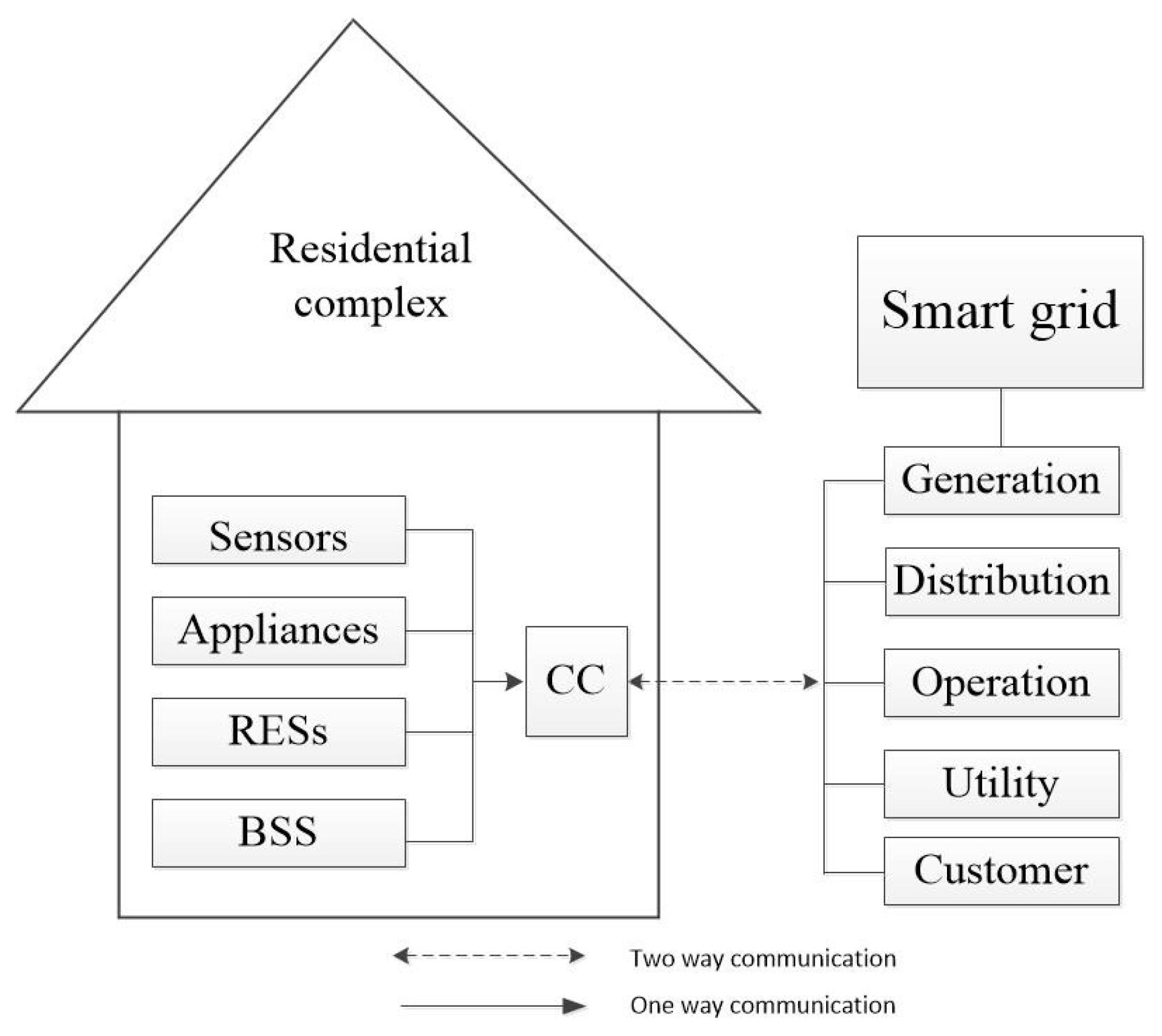
DSM plays a vital role in efficient and reliable operation of SG. Adopting different mechanisms, DSM benefits the end users and utilities under two major functionalities, i.e., efficient energy management and control over the end users’ activities. In the residential sector, each home is equipped with advanced metering infrastructure connected to a central controller in order to ensure stable and optimized energy consumption decisions under two-way communication between utilities and consumers. A conceptual diagram of the proposed DSM mechanism is illustrated in Figure 3. This structure enables users to reduce the electricity bill and the utility to curtail PAR for persistent operation of SG. All appliances request the central scheduler to execute the job, and the scheduler makes the decision about the status of appliances at a particular hour. The scheduler must respect the scheduling horizon provided earlier by users.
Our system model is composed of a smart building of 30 homes in an MG scenario. Each home is equipped with 12 smart appliances, which are to be scheduled within a given time window as shown in Table 1. All appliances must not start before the earliest starting time and finish respective working hours prior to finishing the time horizon. An assumption is made that all users are living with same power consumption habits, and only once a day, an appliance is required to operate. The start and end times of appliances are assumed to be provided by users, whereas other parametric values are listed in Table 1 [32]. Figure 2 shows the block diagram of the smart building and local generation sources.
A time interval of half an hour is considered because the minimum of one hour operation time for home appliances seems impractical. Some home appliances like the coffee maker and the toaster work for less than one hour a day. All appliances have constant power consumption rates; however, the power consumption cost depends on the number of time intervals an appliance runs and the price of electricity during execution cycle.
In addition to the above, the smart residential building also requires heat demand along with the ground area of 2500 m, calculated using CHP sizer Version 2 software (Oak Ridge, TN, USA) [33]. No electricity from the utility is imported to satisfy the heat demand; instead, the smart building has local DERs, which are to be scheduled according to the heat demand curve. DERs and their respective capacities are assumed to be known, which are listed in Table 2 [28]. The operation and maintenance costs of DERs are based on natural gas and other specifications are:
- a CHP production plant with a 1.2 heat to power ratio.
- a boiler of 120-kW capacity.
- one BSS with charge and discharge efficiencies of 90%.
- a gas connection for the CHP and boiler to run.
- the total payable cost depends on the electricity price, the natural gas price and the operation cost.
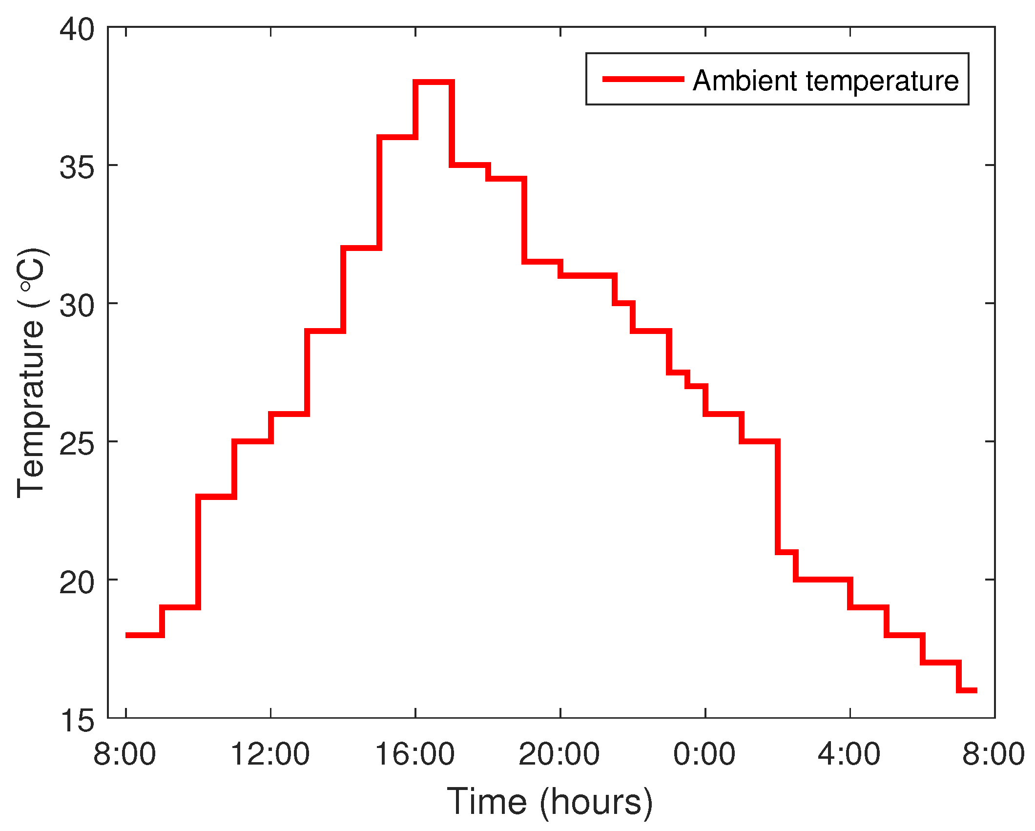
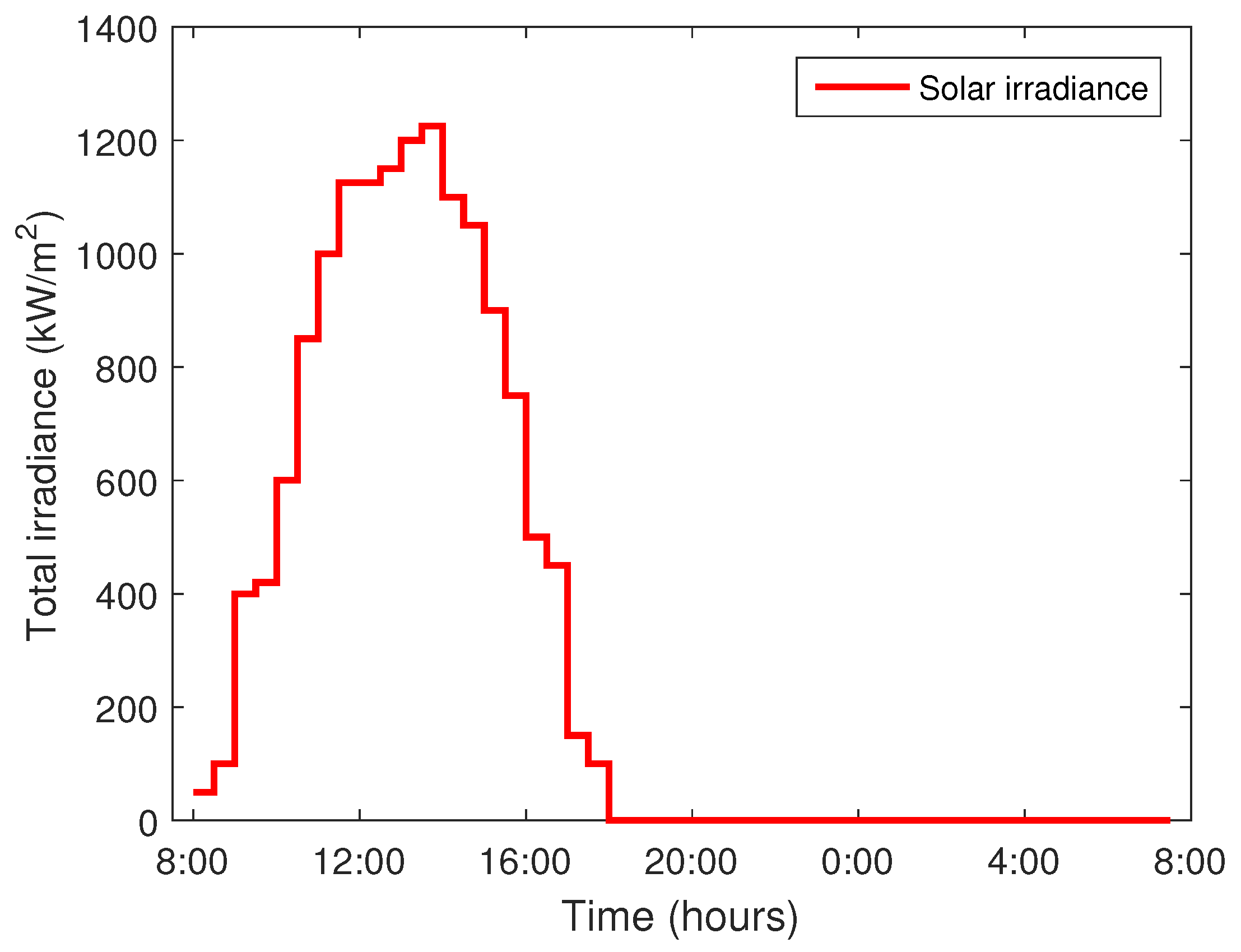
Total electricity demand is satisfied by local generation plus energy imported from the main power grid. BSS is used to store excess electricity generated from RESs and used later when high price hours at the grid or no RE is available. Battery charge and discharge levels under all techniques are shown in Figure 4. RE generation depends on installed capacity, ambient temperature and solar radiations. The profile for ambient temperature and solar radiation is shown in Figure 5 and Figure 6, respectively, and obtained from Meteonorm 6.1 software (Oak Ridge, TN, USA) for the Islamabad region of Pakistan.
4.1. Power Output of Renewable Energy Sources
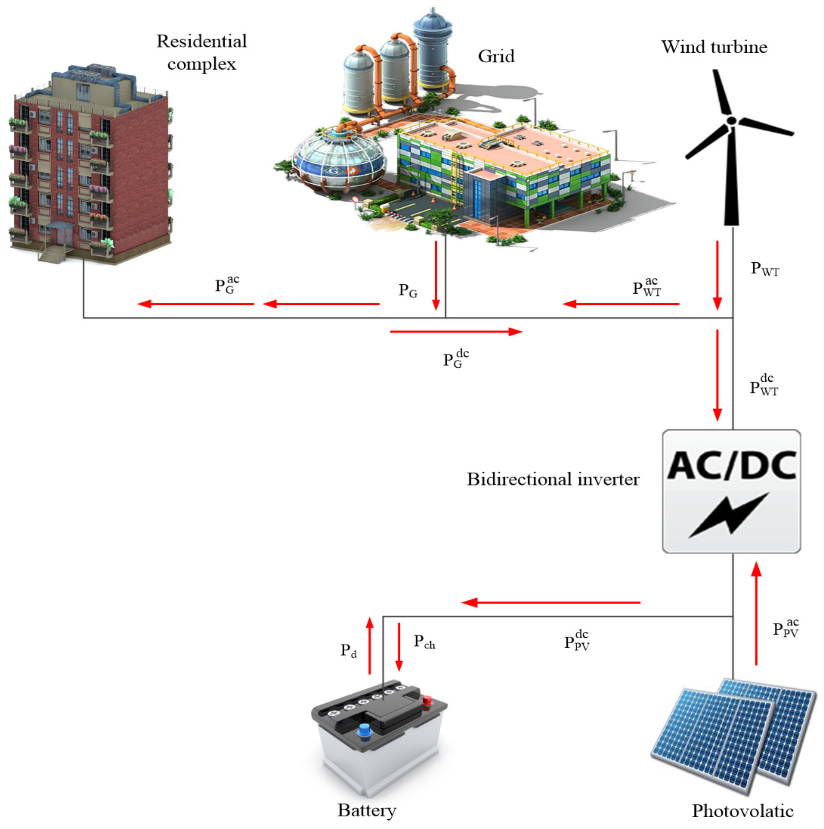
Major RESs include solar and wind; however, PV is the least expensive source of generation and requires one time investment. The planet we live on receives 174,000 terawatts (TW) of solar radiation [34]. The areas with insolation levels of 150–300 W/m or 3.5–7.0 kWh/m per day are the most populated areas in this world [35]. The incoming solar energy (in the form of radiation) that reaches the surface of the Earth is defined as insolation. Approximately 70% of the total radiations are absorbed, and the rest is reflected back to space. This is called the solar energy cascade, which does not have a fixed value around the different locations of the Earth, nor is it constant over different periods of time. If we move to the north and south of the Equator, the insolation shows a continuously varying trend, and its quantity keeps decreasing towards the poles with respect to season. In March and September, the isolations are at the highest level in the Northern Hemisphere, whilst the Southern Hemisphere enjoys September and March [36]. Thus, the power output of RESs depends on several parameters. Some of them are nature dependent, while others can be adjusted accordingly. The former includes season (summer or winter), weather (sunny or cloudy) and topographical constraints, whereas the latter comprises the size and efficiency of installed technologies. A block diagram of the power flow of RESs in the proposed model is shown in Figure 7.
Power output from the PV unit can be measured as a function of solar irradiation and ambient temperature. Both solar irradiance and temperature highly depend on weather and season. A solar panel consists of several cells, which are coupled together to produce power. In a similar work [37], the authors use renewable energy generation and storage systems, where deterministic and stochastic methods have been used to consider uncertainties.
The temperature of a cell can be given as [15]:
where belongs to the temperature of cell (°C) at time t, denotes the current temperature (°C) at given location, is the global solar irradiance (kWh/m), NOCT is the nominal operating cell temperature (°C), which can be defined as a level of temperature reached under the following conditions: irradiance = 800 w/m, air temperature = 20 °C, wind velocity = 1 m/s and tilt angle of cell = 45°. Therefore, the output of a PV array can be measured as [38,39]:
where is the output of the PV at time t, is the derating factor of the PV array, is the standard irradiations (kWh/m) and shows the temperature coefficient (%/°C). The Meteonorm software is used to calculate the radiations on a PV panel of tilt angle 30°, which is considered as the optimal direction for PVs. Generically, if the temperature remains within the limits of 16–36 °C throughout the day and the area of the PV is 200–220 m, then the output power on a typical sunny day would be roughly 500 kW. Moreover, the partially sunny and cloudy days will have 200–300 and 50–70 kW of generation, respectively, under similar conditions.
The power output from a WT is modeled as a piecewise function of wind speed. We denote v as wind speed, as rated wind speed (i.e., where WT generates maximum energy), the cut-in speed (i.e., minimum required speed to turn on WT) and the cut-out speed (i.e., excessive speed, blades brought to test). Besides, the air density, the size of WT obviously effects the total power output. A generic mathematical expression is given below to find output of WT [31]:
The parametric values for , and are 3, 10 and 20, respectively. Users usually do not follow a specific pattern to run daily appliances. Therefore, appliances are categorized according to their electricity consumption pattern in the subsequent section.
4.2. Load Categorization
In view of daily power consumption pattern, appliances are categorized into two groups, i.e., flexible loads and inflexible loads, as described below.
- Inflexible appliances: This type of appliance is also referred to as fixed or regular appliances because of their constant power usage pattern and length of operation time. Typically, inflexible loads include fridge, fan, light, etc., which are considered to be required run loads and cannot be shifted to later hours. These appliances usually do not participate in the DR, so they cannot contribute to the optimization process in order to achieve lower electricity bill. Therefore, regular loads execute their job on respective time slots and have no relation with the appliance scheduler.
- Flexible appliances: Flexible loads are also known as shiftable or burst loads. Flexible appliances include the dish washer, washing machine, spin dryer, etc. The power consumption pattern of this type of appliance can be altered to later hours in response to some incentives. Appliances are shifted to later hours due to two main reasons: either appliances are preferred to alter the consumption pattern from on-peak hours to off-peak hours or when the price for the grid is high, appliances are shifted to low price hours for bill reduction.
4.3. Energy Consumption Model
Each consumer in the smart building has two sets of appliances, discussed earlier, i.e., F and I. The set of flexible appliances and the set of inflexible appliances over a scheduling horizon of . The hourly electricity demand of a single appliance is given as:
where denote electricity demand of an appliance in a respective time slot. The daily electricity consumption of both types of appliances (flexible and inflexible) is given by Equations (5) and (6), respectively:
where denote the power consumption of flexible appliances and represent the power consumption of inflexible appliances at time t. The total daily power consumption is given as:
4.4. Capacity Constraints
The power outputs of considered resources must not exceed beyond the limits of designed capacities:
where , , , , and are the outputs; , and are the capacities of the CHP, boiler, thermal storage, PV, WT and electric storage respectively at t.
4.5. Thermal Storage Constraints
The total heat in the storage at t depends on heat stored at , heat charged and heat discharged. Heat discharged is subject to being subtracted from the total heat because it is the out going source and results in depletion of storage. Heat loss in the process of charging and discharging, i.e., turn around efficiency, is denoted by . In order to store 10 kW in storage, kW must be provided, and in the case of discharging 10 kW of power, kW must be discharged:
where and are the charge and discharge rates of thermal storage at t, respectively. The charge and discharge rates must be within the designed limits of the charge and discharge rates. and are the thermal storage charge and discharge limits:
4.6. Electric Storage Constraints
The total electricity in the electric storage at t depends on the electricity stored at , the electricity charged and discharged. Electricity discharged is subject to being subtracted from the total electricity, because it is the out going source and, hence, results in the depletion of storage. Electricity loss in the process of charging and discharging, i.e., turn around efficiency, is denoted by . The rest of the storage and discharge process is the same as that for heat storage described above:
where and are the charge and discharge rates of electrical storage at time t, respectively. The charge and discharge rates must be within the designed charge and discharge limits. and represent electrical storage charge and discharge limits:
4.7. Energy Balance
The electricity demand is fulfilled by the local RESs, energy drawn from storage minus the energy sent to electrical storage and direct connection of the grid, whereas heat demand is met by the CHP generation, boiler units and heat retrieval from storage minus heat saved in storage. The electricity consumption must not exceed the electricity imported from main grid and the total generation of PV and WT:
where is the processing time duration of appliance k of home i, is the power consumption capacity of appliance k at time period , is a binary variable that shows the status of appliance k at t, is the power output from PV, is the power output from WT at t, and are the electric storage discharge and charge rates and is the total energy imported from the main grid at t. As discussed earlier, the heat demand balance is shown in Equation (21), and is the heat to power ratio of CHP:
4.8. Start and End Time Horizon
Each appliance has to complete its working hours within the given time frame; however, no appliance can start before the provided earliest starting time window, nor can it complete later than finishing time window. Since each appliance has to finish between the given time interval minus the operational time duration, a binary variable is introduced that indicates whether an appliance has finidhed its job or not.
4.9. Power Demand
The maximum electricity demand from the main grid over a period of time is given as:
is the maximum power demand from the power station, and is the energy imported from the grid at t.
4.10. Peak to Average Ratio
The basic aim behind balancing the PAR is to maintain the equilibria of demand and supply between utility and consumers. In our proposed system model, PAR is defined as a ratio of peak load over average load in the given time frame and is symbolized as . Mathematically, PAR can be written as:
4.11. Waiting Time
Inflexible appliances are supposed to run with the highest priority and without any delay, so these appliances do not have any concern with the waiting time. Flexible tasks play a crucial role in the optimization by altering the power consumption behavior. Let and be the start and end times of flexible appliance a, such that ≤ within the given time window interval. In our model, we consider waiting time as discomfort. The more the waiting time is, the lesser the comfort will be. We denote as the working duration and as the actual start time of appliance a. has a value no less than , but less than or equal to given as:
4.12. Objective Function
The objective is to minimize the total power consumption cost of all appliances in the smart residential building. The electricity cost depends on the pricing signal announced by the utility company and the appliances’ power consumption pattern. We have no control over the pricing signal; however, we minimize the cost by altering the power consumption pattern of appliances:
5. Heuristic Techniques
Numerous heuristic, meta-heuristic and mathematical techniques have been used for DSM in the residential sector. Reducing energy expense, reducing PAR, balancing demand and supply, maximizing the user comfort level, stabilizing the grid and ensuring the power quality are some of the objectives of using optimization techniques. One of the key underpinnings of heuristic techniques is that they provide a feasible solution in very low computational time. The workings of TLBO, EDE and our newly-proposed EDTLA are provided below.
5.1. Teaching Learning-Based Optimization
Unlike other evolutionary and swarm-based optimization techniques, TLBO does not have any algorithm-specific parameters. Therefore, parameter tuning is not required, which makes TLBO computationally efficient.
Inspired by the teaching-learning environment of class, TLBO is a population-based algorithm, which is comprised of two phases. The first phase is the teacher phase, while the other is the student phase. In the teacher phase, the best solution (depending on the objective function) of the population is selected as the teacher, and rest act as students. The teacher provides his/her knowledge and tries to change the mean value of the students to raise their level. The following formulas are used to distinguish the level of knowledge of the students and teacher in a particular subject:
where is considered as the outcome of the best learner in respective subject j. The represents a random number whose value is selected between one and two. The teaching factor is represented by , which has a value between one and two. The teaching factor is not the parameter of TLBO, and its value is selected randomly. The formula mentioned in Equation (27b) decides the value of the teaching factor. The updated value of is represented by , and this updated value is selected in the population if it proves to be a better solution than the existing one.
In the second phase, the students interact with each other and learn from the student having more knowledge. A student can only learn from other students in the case that he/she has a lower level of knowledge than that student. In a population of size n, two learners, i.e., M and N, are selected randomly provided that . Since our problem is a minimization problem, so the equation used is:
If the solution provides better results than the existing one, it is selected or else discarded. These updated and accepted values are given to the teacher phase as input in the coming iteration until the termination criterion is satisfied.
5.2. Enhanced Differential Evolution
As the name suggests, EDE is the extended version of the DE algorithm. It has better performance than DE because of fewer control parameters. EDE differs from DE at the stage of generating trial vectors. The population size (NP) and the mutation factor (F) are the two control parameters of EDE. The i-th vector in the current generation of the population is selected as target vector . Therefore, it can be written as:
where D shows the dimensions of the parameter space. Initially, the population is generated randomly between the limits of the upper and lower bounds followed by the mutation step. The mutation steps starts by randomly selecting three distinct vectors from the population. The difference of the two randomly-selected vectors is added to the third vector, and a new mutant vector is formed. The mathematical representation of the mutant vector is shown in Equation (28b) below:
The value of F varies in the range of [0, 2], which explores the search space stepwise. Firstly, 100 iterations are performed, and three groups of trial vectors are generated in each iteration by using the following equations:
Different values of the crossover rate, i.e., 0.3, 0.6 and 0.9, are used to generate the three groups of trial vectors. After mutation, in the selection stage, the fittest group among the three groups of trial vectors is selected to compare with the old population. The most appropriate vector is selected using the equation provided below:
This process continues until the termination criterion is satisfied.
5.3. Enhanced Differential Teaching Learning Algorithm
TLBO is a nature-inspired algorithm influenced by the teaching-learning pattern of a class. Like other evolutionary algorithms, it also works on the principle of repeatedly updating a population of solutions to reach the global best. TLBO consists of two phases, i.e., the teacher phase and the learner phase. In the teacher phase, the teacher tries to provide his/her knowledge to students so that the students can learn and come up to the teacher’s level. Similarly, in the second phase, students interact with each other and continue to learning.
TLBO sometimes suffers from premature convergence and can also get stuck in local minima. To avoid these issues, we incorporate the mutation and crossover steps of the EDE algorithm, which improve the performance and help to search globally. Therefore, two additional steps are added to the TLBO, which are given below.
In the mutation phase, the difference of two randomly-selected vectors is multiplied with the mutation scaling factor and added to a third vector to generate a new mutant vector. All three selected vectors must be different from each other, and the mutation scaling factor (randomly generated number) ranges between zero and one. If the randomly-generated number is less than the crossover rate, the mutant vector is selected in the new population and otherwise discarded. The steps of the hybrid algorithm are provided in Algorithm 1.
| Algorithm 1: Enhanced differential teaching learning algorithm. |
 |
6. Feasible Region of Objective Function
The feasible region of the objective function is shown in Figure 8, which is comprised of six points. The first point is the electricity cost where the minimum load (9 kW) coincides with the minimum price time slot. Similarly, point shows the consumption cost when the minimum load is scheduled in the maximum price time interval. If all appliances are ON in a time interval of maximum price, then the electricity bill is shown by point . Conversely, represents the cost if all appliances are ON in the minimum price time slot. As also mentioned in Section 4, the power consumption is equal to the power rating and status of an appliance at a particular time interval, whereas the electricity cost depends on the power consumption and the price of electricity at that time interval. The RTP signal is announced by the utility, so the power consumption pattern of appliances is modified to reduce the electricity bill. Moreover, in any time slot, the maximum cost of the scheduled case must not exceed the maximum cost of the unscheduled case. Points and show the bounding limits on the maximum load and cost, respectively. The four possible cases of electricity cost are: (i) minimum load, minimum price, (ii) minimum load, maximum price, (iii) maximum load, minimum price, and (iv) maximum load, maximum price.
Feasible Region of Trade-Off
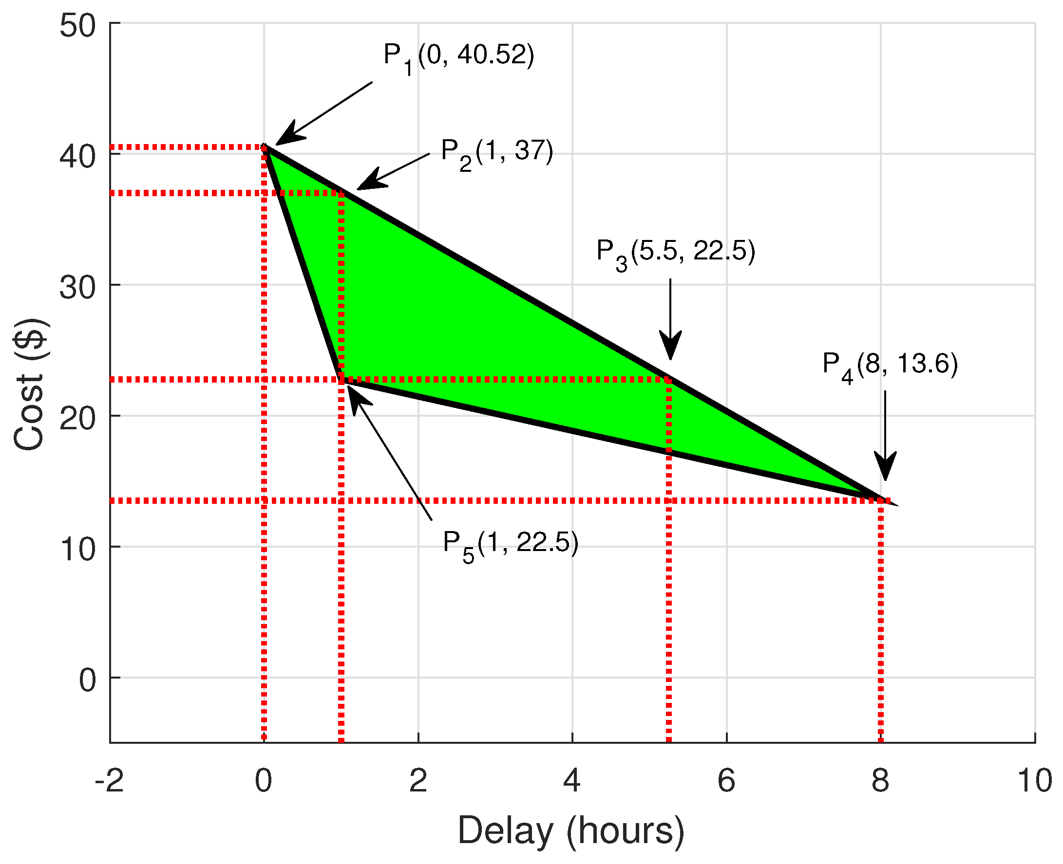
The feasible region of tradeoff between electricity bill and delay is shown in Figure 9. The feasible region consists of five points. shows a point when there is no delay and all appliances run with high priority. The point shows that if we shift our appliance up to 8 h, we pay only 13.6 $ instead of 40.52 $. In our scenario, one hour is the minimum time delay in which a 22.5 $ cost is incurred, as can be seen at point , which is much better than the unscheduled case. Similarly, represents the cost with a similar delay of one hour when appliances power on in a high price hour. If high price hours appear consecutively, then appliances may have to wait for a maximum time of 5.5 h to achieve a similar cost, as depicted by .
7. Simulations and Discussion
In this section, we present simulation findings and comparatively evaluate the workings of GA, TLBO, EDE and our proposed EDTLA under the RTP environment. Subject to a fair comparison, all heuristic techniques are compared with each other and also with the unscheduled case under the same parameters. Our simulations consist of two stages, first without RE integration and the other with RESs and BSS. Total RE generation depends on ambient temperature and the solar radiation profile, which are shown in Figure 5 and Figure 6, respectively. The RTP signal shown in Figure 10 is taken from [11]. The RTP signal, which is assumed to be known ahead, is used, so that users can make informed decisions. We assume 48 time slots of half an hour each from 8 a.m. to 8 a.m. the next day. The performance measuring parameters include: electricity demand, electricity consumption cost, PAR and user discomfort, each of which are discussed hereunder. MATLAB software (2015b, MA, USA) is used for simulations with Intel(R) Core(TM) i3-2370m CPU @ 2.40GHZ @ and 2 GB of RAM on a Windows operating system.
7.1. Electricity Demand
The energy consumption pattern of all appliances under four different techniques is shown in Figure 11. The peak power demand in a specific time interval is about 200 kWh. All techniques perform better than unscheduled, as can be seen in Figure 11. The comparative discussion of electricity demand in four techniques is as follows.
GA schedules most of the appliances either in the early morning or before evening while remaining within the limits of the provided time window. Appliances are scheduled in these slots because of low price hours and only appliances required to run are scheduled in high price hours. GA has better hourly energy consumption during peak price hours than EDE. However, a peak also occurs during Hours 18–19; this is mainly due to the low price hours.
The daily power requirement profile of all appliances under TLBO remains flat throughout the day. This is why TLBO performs well in cost and PAR. TLBO has relatively small power demand during high price hours as compared to other cases. TLBO shows a spike in morning hours; however, it is ignorable because it does not threaten the stability of the grid. The peak power demand in the case of TLBO is 160 kW in Hours 20–21.
EDE mimics the behavior of GA particularly in morning hours and, later unlike GA, EDE has flat curve during the rest of the day. No peak occurs, and appliances are scheduled when the price is minimum. Peak power demand in a specific time interval is 150 kWh, which is better than both GA and TLBO. EDE shows an increasing trend in the morning hours and a decreasing trend in later hours. It schedules most of the appliances during morning hours where the electricity price curve has a moderate behavior. EDE results in a small peak during Hours 7–8, which is mainly due to the low price during this period. However, at the same time, it contributes to lowering the waiting time of appliances. Our proposed technique results in flat behavior during the whole day. EDTLA neither schedules appliances in a high price hour nor creates a peak in the low price hour. It shows a moderate power demand curve due to which it has minimum electricity demand from the main power station in peak hours, i.e., 19–25. Peak power demand in the case of EDTLA is nearly 150 kWh, which is normal in a 30-home scenario.
Additionally, Table 3 shows the total carbon emissions of one day when the total energy is imported from the main grid. In the aforementioned case, there is no RE, and the whole electricity demand is entertained by the main power grid. The smart residential complex generates its own electricity to meet daily electricity demands. When we integrate RE, the power demand curve under all cases becomes flatter, as shown in Figure 12. Half of the total power demand is assumed to be generated by local RESs of the residential complex. Figure 13 shows an estimated RE generation on the simulation day. Most of the appliances are scheduled when adequate RE is available. Excess RE is stored in BSS and used later when there is no local energy generation or a high electricity price at the grid. There is no or very low electricity demand in the initial hours of the day due to the availability of local energy, particularly in the case of TLBO and EDTLA. Consequently, RE integration contributes to lowering the electricity bill and a flat PAR. EDTLA has shown the best demand curve in both cases with minimum electricity demand from the main power grid. During the whole day, when the price is high, EDTLA has no electricity demand from the grid. EDTLA satisfies load demand from local generation and BSS when there is a peak at the grid side. EDE does not perform better in terms of hourly power demand as compared to GA; however, when RESs are integrated, EDE has a lower electricity bill. This is because of the low power demand in high price hours. From the above results, it can be seen that EDTLA has a more appropriate and flat demand curve among all algorithms. Similarly, Table 4 lists the percentage decrease in carbon emissions when RESs and BSS are incorporated. It is proven that integration of RESs leads to significantly lowering of the carbon emissions and other harmful gasses.
7.2. Electricity Cost
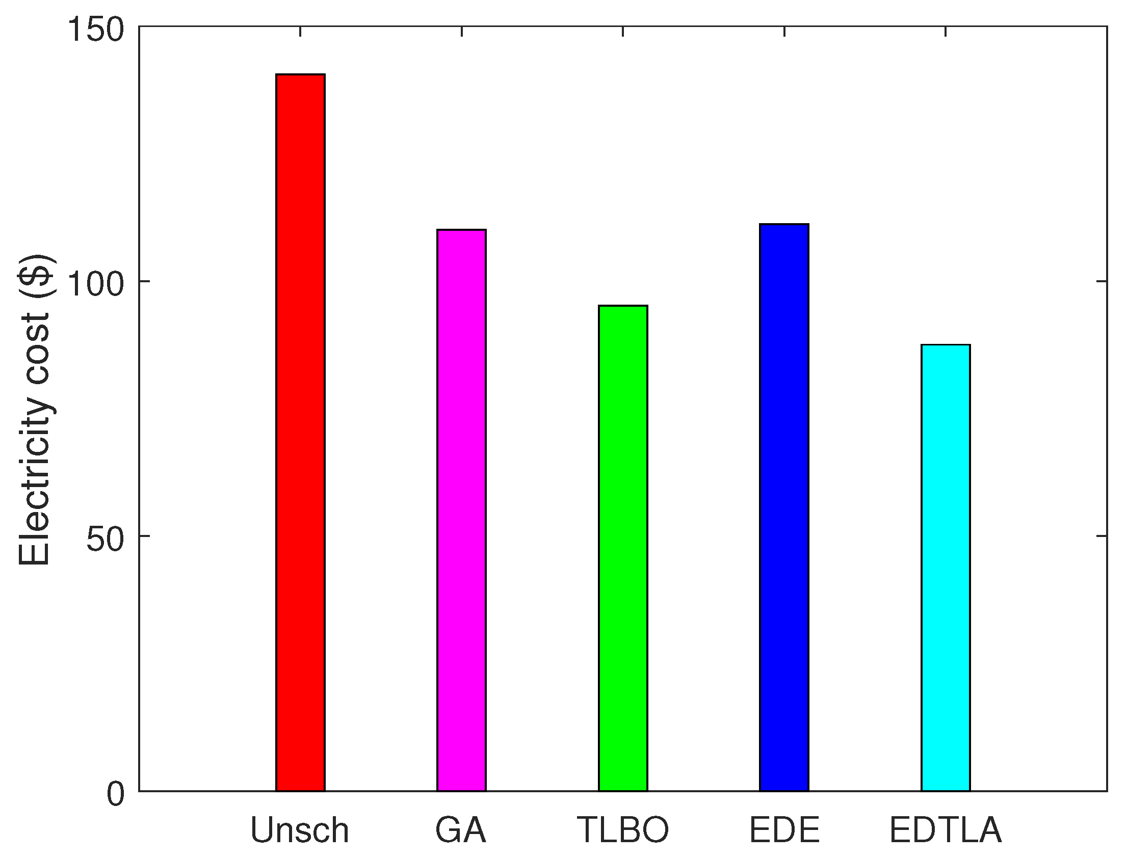
Figure 14 shows the comparison of the hourly power consumption cost of the aforementioned techniques without the integration of BSS and RESs. EDE shows some spikes; however, their impact on total cost is negligible because these spikes last for one or a couple of low price time intervals. GA has a maximum of an 8 $ cost in any single time interval, which is adequately less than the unscheduled case. On the other hand, TLBO has a flat curve during the whole day, because it utilizes low price hours. Initially, all techniques show an average behavior towards cost; however, TLBO increases drastically later when there is a low price hour, but only for one time slot. EDE and GA schedule appliances in high peak hours, which consequently decrease the waiting time, but at the cost of the increased consumption expenditures. EDE does not schedule appliances during time slots 10–20, which as a result creates a peak later in the high price time slots; due to which, EDE has the highest total electricity cost among the four techniques, as can be seen in Figure 15. GA and EDE have comparable costs of consumption; however, GA performs slightly better. Our proposed EDTLA shows a flat behavior of power consumption throughout the day, so its power consumption cost is minimum among all algorithms in both cases. The total electricity bill for one day is 135.88 $, 116.37 $, 89.47 $, 118.66 $ and 82.14 $ in the case of unscheduled, GA, TLBO, EDE and EDTLA, respectively. The percentage reduction of cost in the two scenarios under all techniques is shown in Table 3 and Table 4.
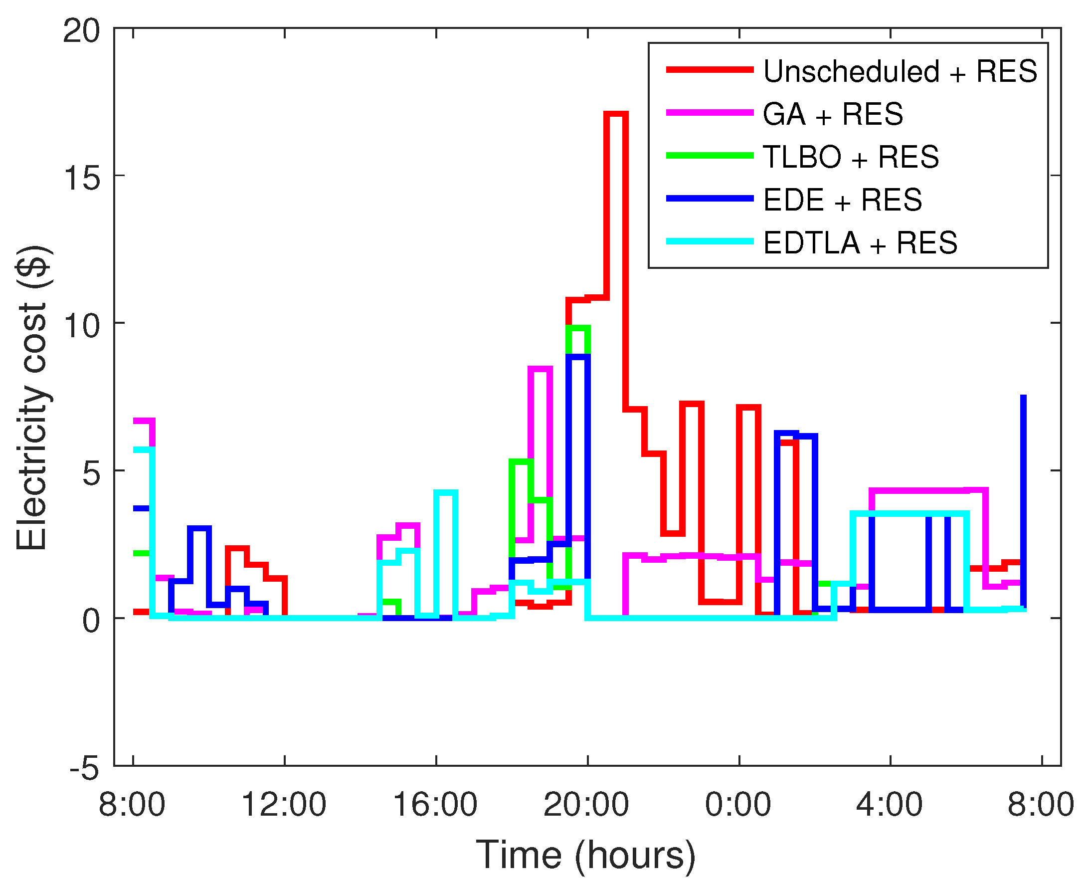
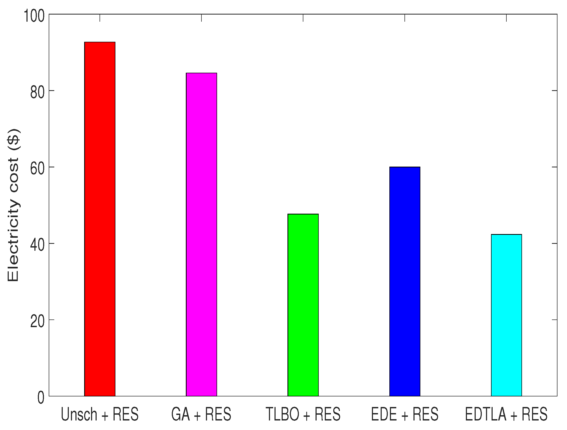
In the second scenario, where RESs and BSS are also available, the maximum cost in one time slot decreases to 9 $ in the case of TLBO. This decrease is due to the discharge of BSS when the peak occurs at the grid, as also shown in Figure 4. On the other hand, the maximum cost in one time interval remains the same under GA and TLBO because the RE and BSS are used in high price hours (i.e., 24–27), where all techniques have nearly zero cost of electricity from the grid. Figure 16 depicts the hourly cost of electricity obtained from the grid after using local RESs and BSS. Total per day cost in both cases (with and without RESs and BSS) is shown in Figure 15 and Figure 17, respectively. The total electricity bill for one day is 92.63 $, 84.24 $, 48.11 $, 62.21 $ and 44.83 $ in the case of unscheduled, GA, TLBO, EDE and EDTLA, respectively, when RESs and BSS are also available. EDTLA performs better in terms of cost with a reduction of 8% in the total electricity bill as compared to TLBO and 36% as compared to the unscheduled case. From the above figures and facts, the impact of RESs and BSS can easily be noted, and with a small one time investment on RESs and BSS, the user can reduce the electricity bill and PAR. The summarized results are also shown in Table 4.
7.3. Peak to Average Ratio
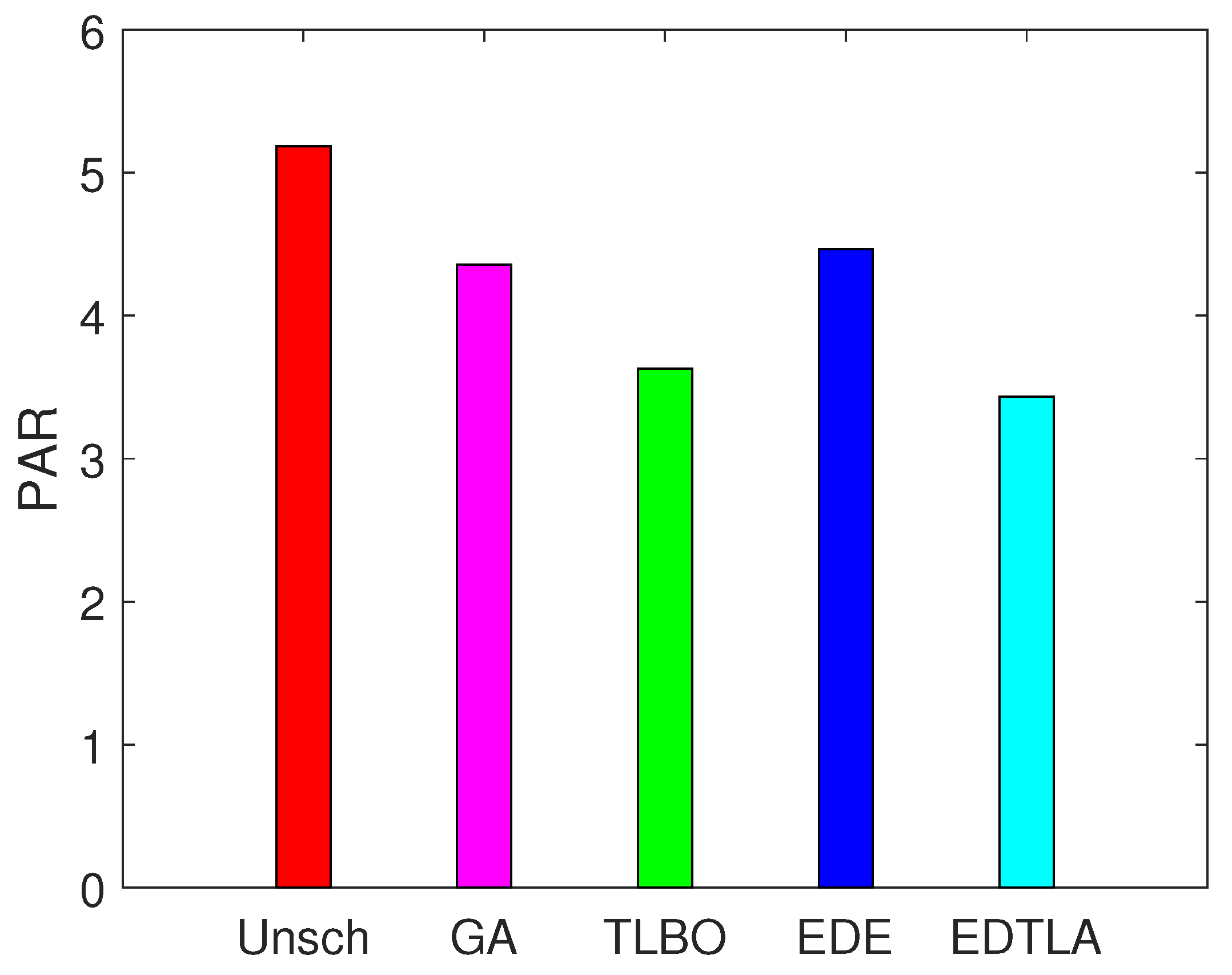
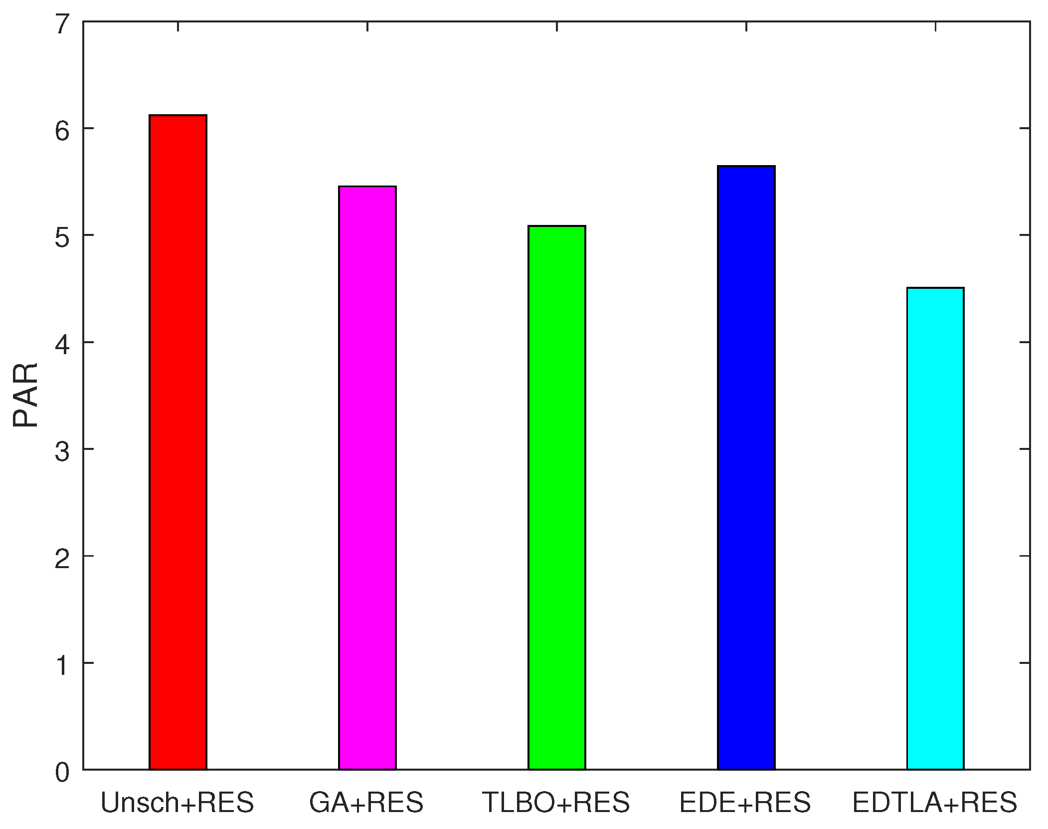
The performance of four different heuristic techniques assessed in terms of PAR is shown in Figure 18. It is clear that scheduling with GA, TLBO, EDE and EDTLA leads towards low PAR as compared to the unscheduled case. When RESs and BSS are integrated, the peak at any hour is reduced up to a significant level; however, PAR becomes high, due to very minimal average load at the grid. The major portion of load is shifted to RESs, and approximately half remains on the grid side. Peak load remains the same in GA and TLBO when RESs are integrated; whereas, the average load becomes flat. Therefore, the PAR shows an increasing trend when RESs are added, as can be seen in Figure 19. When peak demand occurs at the grid side, BSS is used at the consumer premises to reduce the load at the grid side. The battery is charged when the RE is available and discharged later when no RE is available, as shown in Figure 4. The EDE has the highest PAR among the scheduling algorithms because it creates several small peaks in low price hours, as also shown in Figure 11. GA creates a moderate peak, so it shows moderate PAR.
As also shown in Figure 12, TLBO has a flat pattern during the whole day except Interval 20, so its PAR is minimum among all algorithms, which is approximately 3.6; whilst our proposed algorithm further decreases the PAR and achieves 5% more efficient results as compared to TLBO. Table 3 and Table 4 show the percent decrease in the value of PAR with and without RES integration in comparison with the unscheduled case. Results illustrate that the integration of RESs and BSS not only enhances the grid stability, but also reduces the daily electricity expenditure.
7.4. User Discomfort
User discomfort is calculated in terms of the time delay of appliances from the given earliest starting time window. A tradeoff is always seen in user comfort and electricity cost, described later in the upcoming subsection. The electricity bill shows a decreasing trend with a compromise on comfort, and opposite case is also true. Figure 20 shows the waiting time of all appliances under four different heuristic techniques. It can be clearly seen that EDE has minimum delay, which means least discomfort, however at the cost of a huge electricity bill, as depicted in Figure 15. Most of the appliances do not wait to execute in the case of the EDE algorithm. GA and TLBO have comparable waiting time and appliances, which allow one to shift time intervals, wait and contribute to the electricity bill reduction. EDTLA has more waiting time than the TLBO technique, which is mainly due to convergence towards the global optimal solution. TLBO schedules appliances as it finds the minimum price time slot; however, our proposed technique completely searches all possible solutions and then schedules accordingly. When we integrate RESs and BSS, there is no direct impact on user comfort in terms of delay; however, the user is satisfied when the electricity bill shows a decreasing trend. In the unscheduled case, appliances run whenever they are required, regardless of the cost and grid stability concerns, so no user comfort is calculated in the unscheduled case.
7.5. Heat Demand
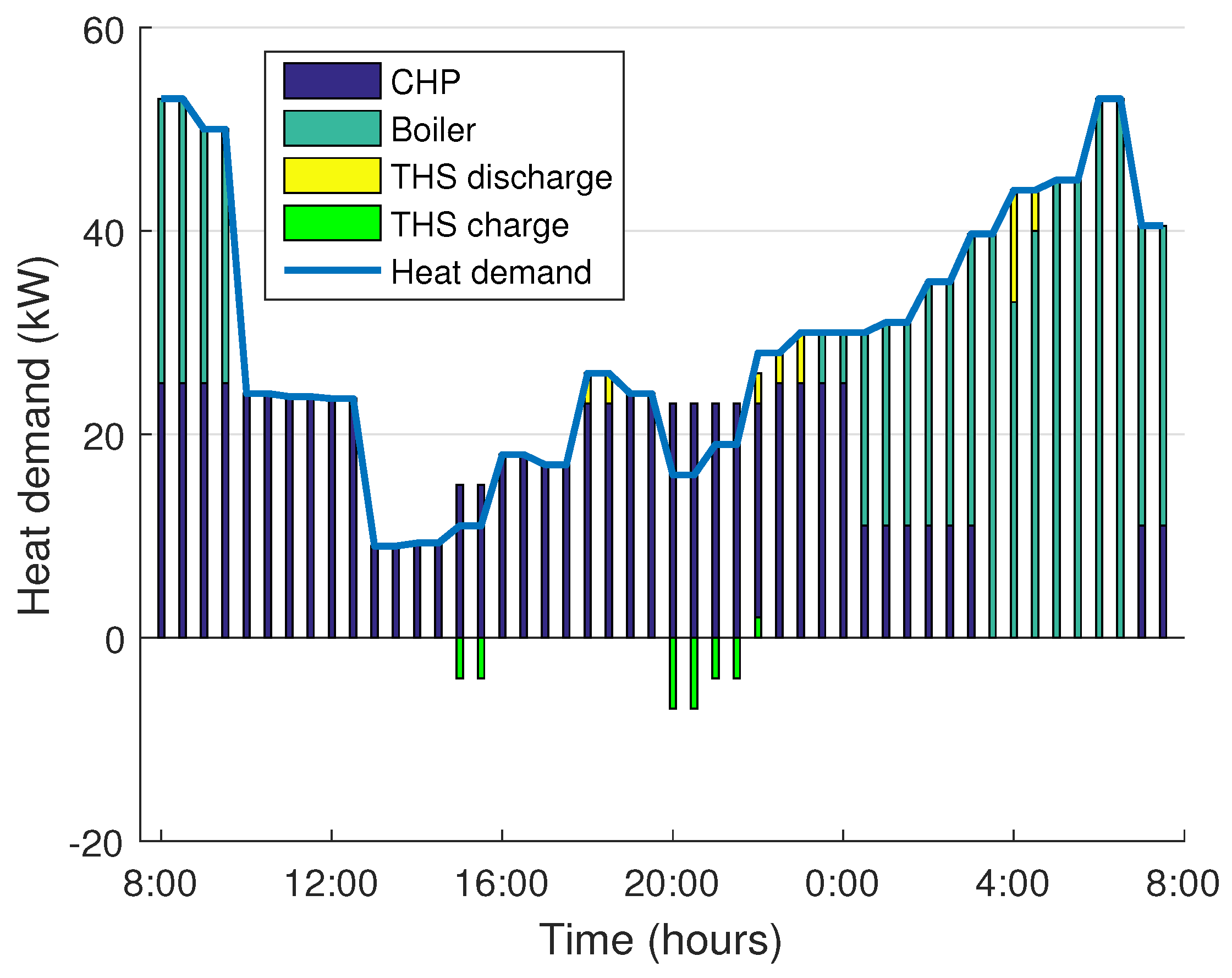
Figure 21 presents the heat balance for smart building. Heat is provided by using local resources of the smart building, which consequently decrease global carbon emissions. The heat demand curve has two peak demands: first, early in the morning; and the other is later, when the temperature becomes low. During these peak hours, the CHP generator constantly works at full capacity due to more heat demand, and the rest of the heat is either provided by thermal storage or the boiler. The boiler starts generating more heat to fulfill the demand when the price becomes flat and no heat is harvested from the CHP generators. CHP does not generate excess power unless and until the generated heat is utilized or saved in storage. Thermal storage works as a heat backup and cannot save more heat than its designed storage capacity. Storage is charged when excess power is available and discharged when required. Since the heat demand curve is given, only resources are scheduled in this case in order to lower the carbon emissions and total payable expenditures.
7.6. Execution Time and Performance Tradeoffs
The execution overheads of four heuristic techniques under two different cases are listed in Table 5. In the first case, GA, TLBO and EDE require 3.41, 8.01, and 1.2 s, whereas in the second case, the time jumps to 4.6, 8.24 and 2.4 s, respectively. EDE consumes the minimum time in order to provide desirable results because of good convergence characteristics and fewer control parameters. TLBO requires more execution time because of the continuous teaching-learning process. Our proposed hybrid algorithm requires 8.9 and 9.9 s to finish the job. EDTLA consumes more time to find the optimal solution and to avoid premature convergence.
From the above results and discussions, it is proven that all techniques are able to schedule appliances in a way that reduces the electricity bill and the PAR and that maintains the load profile, especially when RESs and BSS are incorporated. Besides this, none of the techniques is perfect in all performance metrics. A tradeoff can be seen in Figure 15 and Figure 20, where EDE has the minimum delay (i.e., higher comfort), however at the cost of a higher electricity bill. Similarly, in Figure 15, GA has a moderate electricity bill; however, PAR is highest among all scheduling techniques, as shown in Figure 18. Our scheduling algorithm outperforms the other three heuristic methods in terms of electricity bill and PAR at the cost of slightly high execution overhead. Homogenous tradeoffs exist when RESs and BSS are incorporated in the scenario described above.
8. Life Cycle Energy Analysis
The life cycle analysis approach is used to estimate all energy input in its life cycle. Generally, the boundaries of life cycle analysis include the energy use in the manufacturing/process, use and demolition phases. The manufacturing phase includes the energy used for the transportation of building material, installation of technical equipment and renovation. The operation phase includes all of the activities related to the use of that building, maintaining comfort in terms of heating, cooling, water supply, security, etc. The last phase involves the activities related to the destruction of buildings, transportation of dismantled material from one place to other place or to recycling plants. From this discussion, it can be concluded that energy is required in each phase of a building from cradle to grave. In this work, we do not consider the cost of manufacturing and demotion phases.
9. Conclusions and Future Work
This paper proposes an EMM to optimally schedule residential load to lower the electricity bill, user discomfort and carbon emissions in an nZEB. For this purpose, we used the optimization algorithms GA, TLBO and EDE for scheduling to validate the proposed nZEB concept. In addition, after analyzing the performance of these optimization algorithms, a hybrid algorithm is also proposed for further improvement in the already achieved results; using cost, PAR, user comfort and total amount of carbon emissions as performance parameters (Table 3 and Table 4). However, along with the simulation results, the feasible regions of the proposed objective functions have also been calculated to validate the results. In this work, two cases are considered: (i) without integration of RES; and (ii) with integration of RES. The former one reduces the electricity cost and PAR up to 36% and 43%, respectively; while the later one reduces electricity cost, PAR and carbon emissions up to 67%, 29% and 55%, respectively, showing the difference between traditional energy management and ZEB techniques. The proposed model is generic and can be extended to any number of residential units; homes, buildings, etc.
The future work would include power trading among multiple homes, MGs and EVs under a large share of RESs.
Acknowledgments
This project was full financially supported by the King Saud University, through the Vice Deanship of Research Chairs.
Author Contributions
Nadeem Javaid, Sardar Mehboob Hussain, and Ibrar Ullah proposed, implemented, and wrote the optimization schemes. Muhammad Asim Noor, Abdul Wadood, Ahmad Almogren, and Atif Alamri wrote technical sections of the manuscript. All authors refined the manuscript and responded to the queries of the respected reviewers.
Conflicts of Interest
The authors declare no conflicts of interest.
References
- Sesana, M.M.; Salvalai, G. Overview on life cycle methodologies and economic feasibility for nZEBs. Build. Environ. 2013, 67, 211–216. [Google Scholar] [CrossRef]
- Torcellini, P.; Pless, S.; Deru, M.; Crawley, D. Zero Energy Buildings: A Critical Look at the Definition; National Renewable Energy Laboratory and Department of Energy: Golden, CO, USA, 2006. [Google Scholar]
- Marszal, A.J.; Heiselberg, P.; Bourrelle, J.S.; Musall, E.; Voss, K.; Sartori, I.; Napolitano, A. Zero Energy Building—A review of definitions and calculation methodologies. Energy Build. 2011, 43, 971–979. [Google Scholar] [CrossRef]
- Bisegna, F.; Burattini, C.; Manganelli, M.; Martirano, L.; Mattoni, B.; Parise, L. Adaptive control for lighting, shading and HVAC systems in near zero energy buildings. In Proceedings of the 2016 IEEE 16th International Conference on Environment and Electrical Engineering (EEEIC), Florence, Italy, 7–10 June 2016; pp. 1–6. [Google Scholar]
- Ghalebani, A.; Das, T.K. Design of Financial Incentive Programs to Promote Net Zero Energy Buildings. IEEE Trans. Power Syst. 2017, 32, 75–84. [Google Scholar] [CrossRef]
- Peterson, K.; Torcellini, P.; Grant, R.; Taylor, C.; Punjabi, S.; Diamond, R. US Department of Energy. Available online: http://energy.gov/sites/prod/files/2015/09/f26/A%20Common%20Definition%20for%20Zero%20Energy%20Buildings.pdf (accessed on 13 January 2017).
- Voss, K.; Musall, E.; Sartori, I.; Lollini, R. Nearly Zero, Net Zero, and Plus Energy Buildings-Theory, Terminology, Tools, and Examples. Transit. Renew. Energy Syst. 2013, 875–889. [Google Scholar] [CrossRef]
- Lo, C.-H.; Ansari, N. The progressive smart grid system from both power and communications aspects. IEEE Commun. Surv. Tutor. 2012, 14, 799–821. [Google Scholar] [CrossRef]
- Akhtar, Z.; Saqib, M.A. Microgrids formed by renewable energy integration into power grids pose electrical protection challenges. Renew. Energy 2016, 99, 148–157. [Google Scholar] [CrossRef]
- Rasheed, M.B.; Javaid, N.; Ahmad, A.; Khan, Z.A.; Qasim, U.; Alrajeh, N. An Efficient Power Scheduling Scheme for Residential Load Management in Smart Homes. Appl. Sci. 2015, 5, 1134–1163. [Google Scholar] [CrossRef]
- Ma, K.; Yao, T.; Yang, Y.; Guan, X. Residential power scheduling for demand response in smart grid. Int. J. Electr. Power Energy Syst. 2016, 78, 320–325. [Google Scholar] [CrossRef]
- Samadi, P.; Wong, V.W.S.; Schober, R. Load scheduling and power trading in systems with high penetration of renewable energy resources. IEEE Trans. Smart Grid 2016, 7, 1802–1812. [Google Scholar] [CrossRef]
- Hakimi, S.M.; Moghaddas-Tafreshi, S.M. Optimal planning of a smart microgrid including demand response and intermittent renewable energy resources. IEEE Trans. Smart Grid 2014, 5, 2889–2900. [Google Scholar] [CrossRef]
- Garcia, J.A.M.; Martin, A.J.G. Optimal distributed generation location and size using a modified teaching–learning based optimization algorithm. Int. J. Electr. Power Energy Syst. 2013, 50, 65–75. [Google Scholar] [CrossRef]
- Atia, R.; Yamada, N. Sizing and analysis of renewable energy and battery systems in residential microgrids. IEEE Trans. Smart Grid 2016, 7, 1204–1213. [Google Scholar] [CrossRef]
- Sartori, I.; Napolitano, A.; Voss, K. Net zero energy buildings: A consistent definition framework. Energy Build. 2012, 48, 220–232. [Google Scholar] [CrossRef]
- Mathiesen, B.V.; Lund, H.; Connolly, D.; Wenzel, H.; Østergaard, P.A.; Möller, B.; Nielsen, S.; Ridjan, I.; Karnøe, P.; Sperling, K.; et al. Smart Energy Systems for coherent 100% renewable energy and transport solutions. Appl. Energy 2015, 145, 139–154. [Google Scholar] [CrossRef]
- Lv, T.; Ai, Q. Interactive energy management of networked microgrids-based active distribution system considering large-scale integration of renewable energy resources. Appl. Energy 2016, 163, 408–422. [Google Scholar] [CrossRef]
- Rahbar, K.; Xu, J.; Zhang, R. Real-time energy storage management for renewable integration in microgrid: An off-line optimization approach. IEEE Trans. Smart Grid 2015, 6, 124–134. [Google Scholar] [CrossRef]
- Li, T.; Dong, M. Real-time residential-side joint energy storage management and load scheduling with renewable integration. IEEE Trans. Smart Grid 2016. [Google Scholar] [CrossRef]
- Truong, N.X.; Tung, N.L.; Hung, N.Q.; Delinchant, B. Grid-connected PV system design option for nearly zero energy building in reference building in Hanoi. In Proceedings of the IEEE International Conference on Sustainable Energy Technologies (ICSET), Hanoi, Vietnam, 14–16 November 2016; pp. 326–331. [Google Scholar]
- Rahim, S.; Javaid, N.; Ahmad, A.; Khan, S.A.; Khan, Z.A.; Alrajeh, N.; Qasim, U. Exploiting heuristic algorithms to efficiently utilize energy management controllers with renewable energy sources. Energy Build. 2016, 129, 452–470. [Google Scholar] [CrossRef]
- Rasheed, M.B.; Javaid, N.; Awais, M.; Khan, Z.A.; Qasim, U.; Alrajeh, N.; Iqbal, Z.; Javaid, Q. Real time information based energy management using customer preferences and dynamic pricing in smart homes. Energies 2016, 9, 542. [Google Scholar] [CrossRef]
- Zhang, Y.; Rahbari-Asr, N.; Duan, J.; Chow, M.Y. Day-Ahead Smart Grid Cooperative Distributed Energy Scheduling With Renewable and Storage Integration. IEEE Trans. Sustain. Energy 2016, 7, 1739–1748. [Google Scholar] [CrossRef]
- Chapman, A.C.; Verbič, G.; Hill, D.J. Algorithmic and strategic aspects to integrating demand-side aggregation and energy management methods. IEEE Trans. Smart Grid 2016, 7, 2748–2760. [Google Scholar] [CrossRef]
- Moradi, M.H.; Abedini, M.; Tousi, S.R.; Hosseinian, S.M. Optimal siting and sizing of renewable energy sources and charging stations simultaneously based on Differential Evolution algorithm. Int. J. Electr. Power Energy Syst. 2015, 73, 1015–1024. [Google Scholar] [CrossRef]
- Bahrami, S.; Wong, V.W.; Huang, J. An Online Learning Algorithm for Demand Response in Smart Grid. IEEE Trans. Smart Grid 2017. [Google Scholar] [CrossRef]
- Zhang, D.; Evangelisti, S.; Lettieri, P.; Papageorgiou, L.G. Economic and environmental scheduling of smart homes with microgrid: DER operation and electrical tasks. Energy Convers. Manag. 2016, 110, 113–124. [Google Scholar] [CrossRef]
- Mahmood, D.; Javaid, N.; Ahmed, S.; Ahmed, I.; Niaz, I.A.; Abdul, W.; Ghouzali, S. Orchestrating an Effective Formulation to Investigate the Impact of EMSs (Energy Management Systems) for Residential Units Prior to Installation. Energies 2017, 10, 335. [Google Scholar] [CrossRef]
- Rasheed, M.B.; Javaid, N.; Ahmad, A.; Awais, M.; Khan, Z.A.; Qasim, U.; Alrajeh, N. Priority and delay constrained demand side management in real-time price environment with renewable energy source. Int. J. Energy Res. 2016, 40, 2002–2021. [Google Scholar] [CrossRef]
- Wu, T.; Yang, Q.; Bao, Z.; Yan, W. Coordinated energy dispatching in microgrid with wind power generation and plug-in electric vehicles. IEEE Trans. Smart Grid 2013, 4, 1453–1463. [Google Scholar] [CrossRef]
- Domestic Electric Energy Usage. Electropedia. Available online: http://www.mpoweruk.com/electricity_demand.htm (accessed on 27 March 2017).
- Action Energy. CHP Sizer Version 2; The Carbon Trust: London, UK, 2017. [Google Scholar]
- Solar Energy and Radditions. Available online: https://www.en.wikipedia.org/wiki/Solar_energy (accessed on 27 March 2017).
- Ahmad, A.; Khan, A.; Javaid, N.; Hussain, H.M.; Abdul, W.; Almogren, A.; Alamri, A.; Niaz, I.A. An Optimized Home Energy Management System with Integrated Renewable Energy and Storage Resources. Energies 2017, 10, 549. [Google Scholar] [CrossRef]
- Insolation Level and Atmosphere. Available online: http://coolgeography.co.uk/A-level/AQA/Year%2013/Weather%20and%20climate/Climate%20controls/Insolation%20and%20the%20atmosphere.htm (accessed on 29 June 2017).
- Wang, Y.; Wang, B.; Chu, C.C.; Pota, H.; Gadh, R. Energy management for a commercial building microgrid with stationary and mobile battery storage. Energy Build. 2016, 116, 141–150. [Google Scholar] [CrossRef]
- Patel, R.M. Wind and Solar Power Systems: Design, Analysis, and Operation, Second Edition; CRC Press: New York, NY, USA, 2006. [Google Scholar]
- Shirazi, E.; Jadid, S. Optimal residential appliance scheduling under dynamic pricing scheme via HEMDAS. Energy Build. 2015, 93, 40–49. [Google Scholar] [CrossRef]
Figure 1.
Graphical representation of nearly zero energy building (nZEB) balance concept.
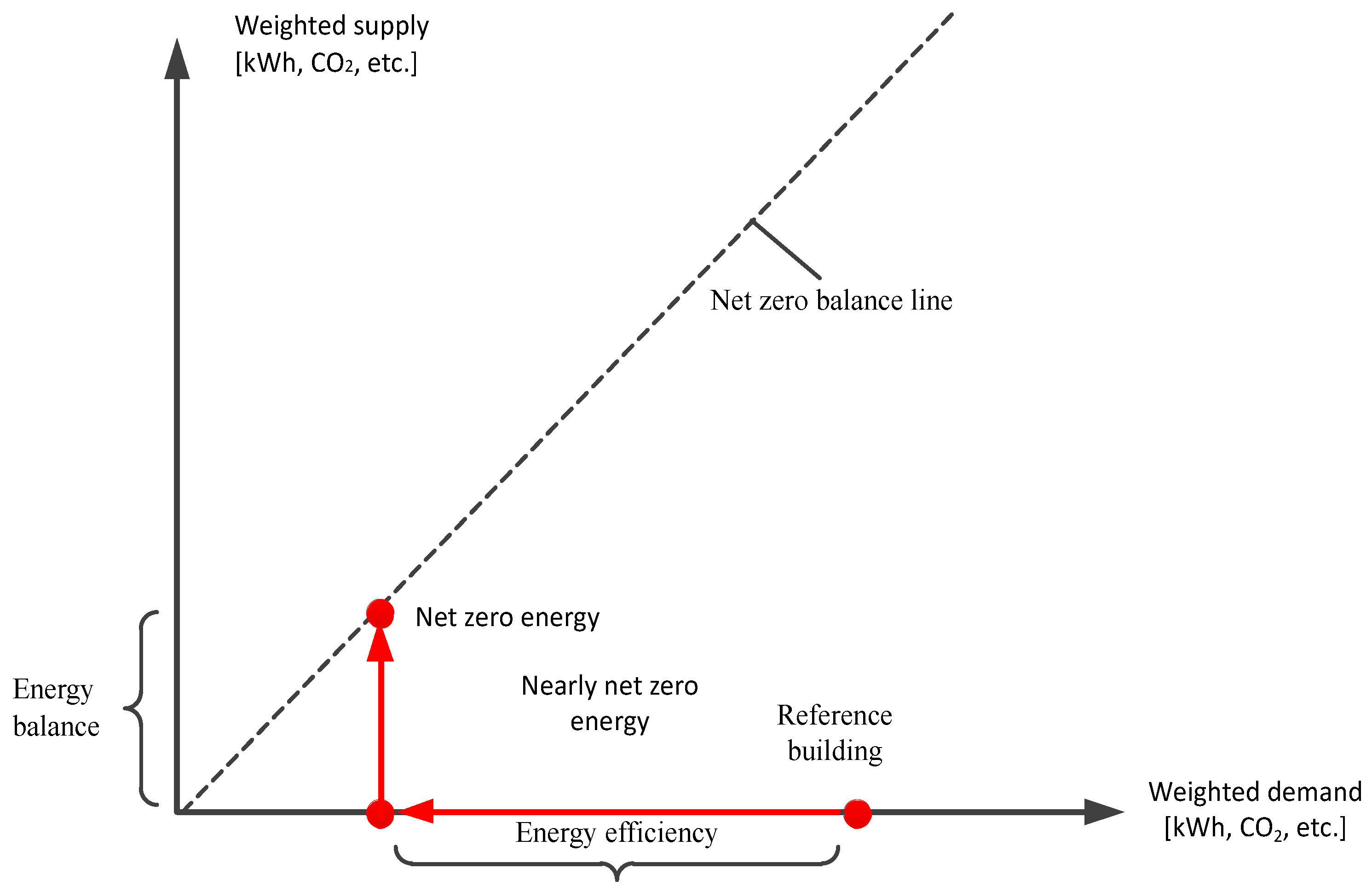
Figure 2.
Smart residential complex.
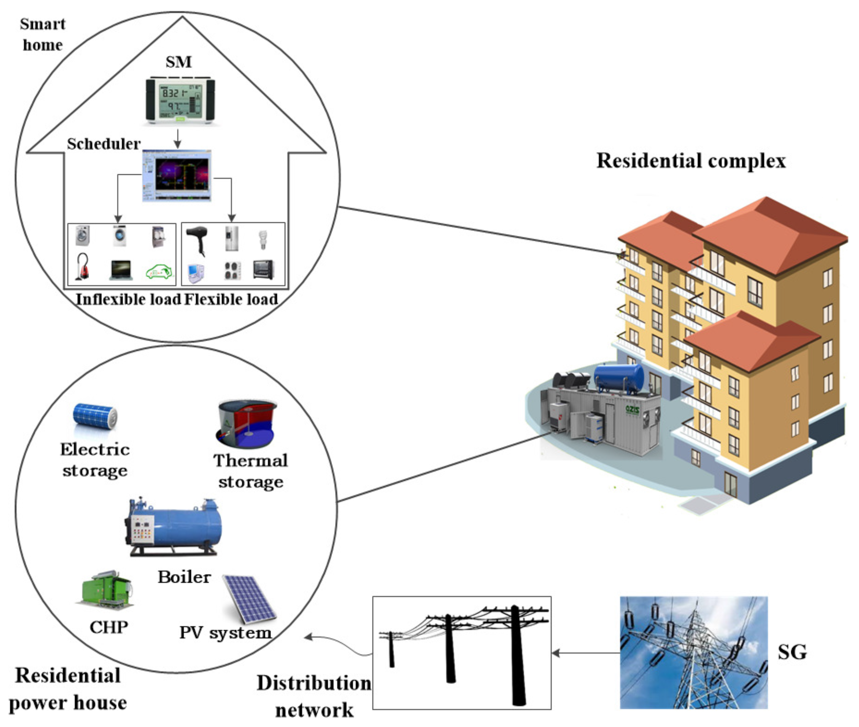
Figure 3.
Architecture of the proposed demand side management (DSM).

Figure 4.
Battery charge and discharge levels.
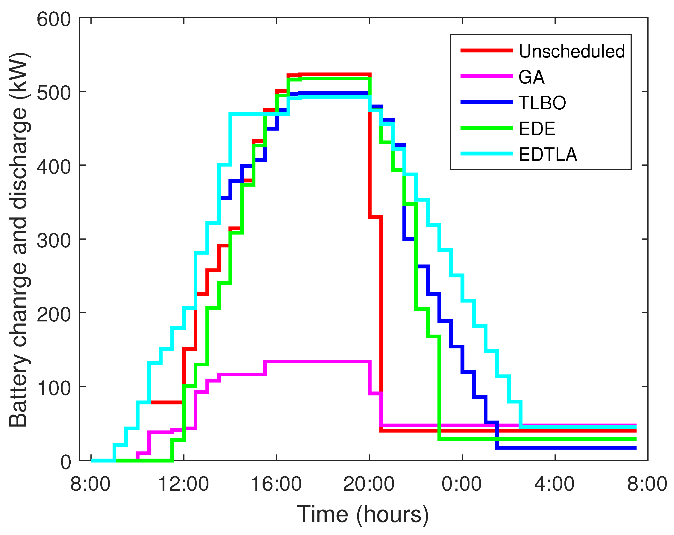
Figure 5.
Ambient temperature.

Figure 6.
Estimated solar radiations.

Figure 7.
Power flow of renewable energy sources (RESs) in the proposed model.

Figure 8.
Feasible region of objective function.
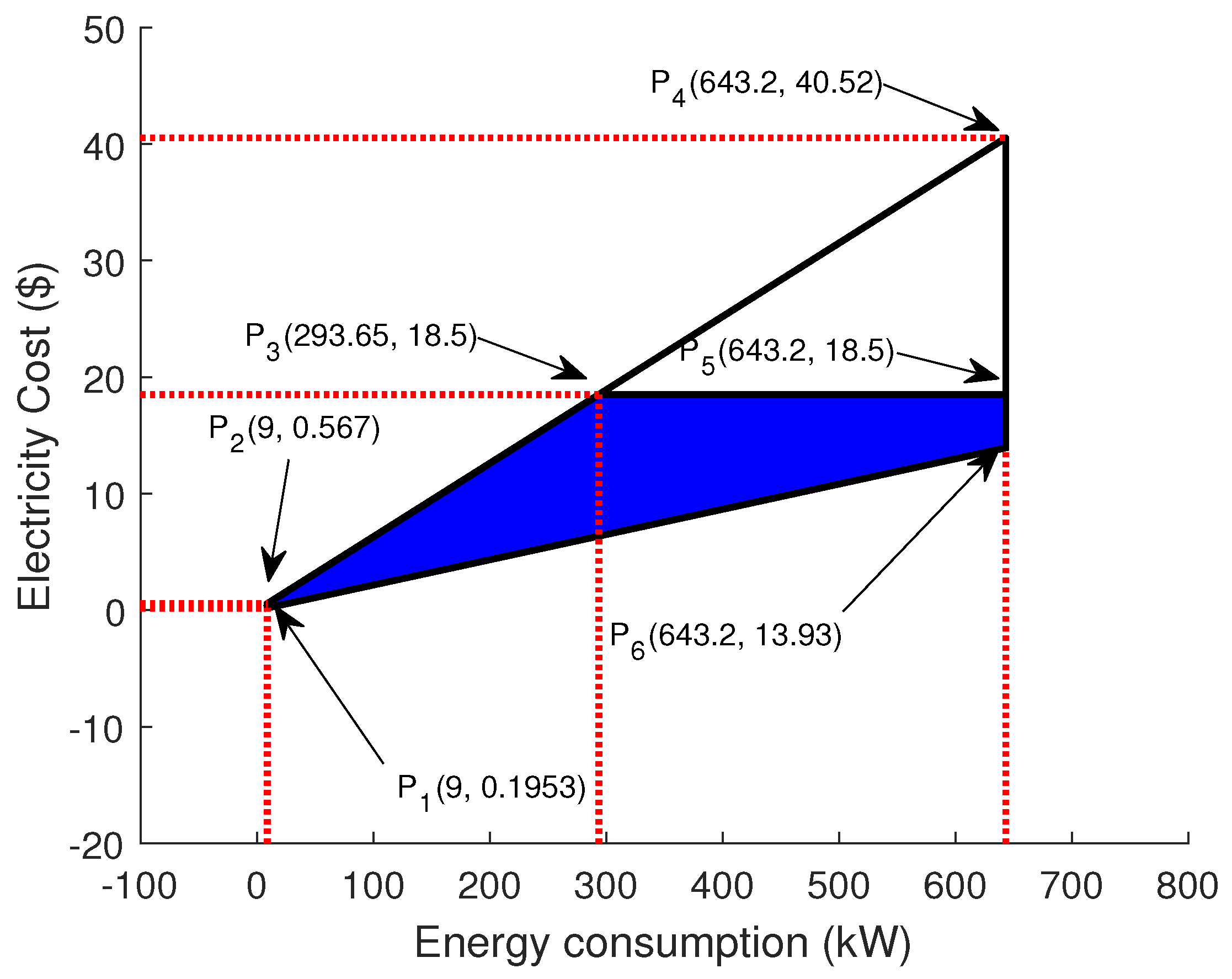
Figure 9.
Feasible region of tradeoff.

Figure 10.
Real time porice signal.
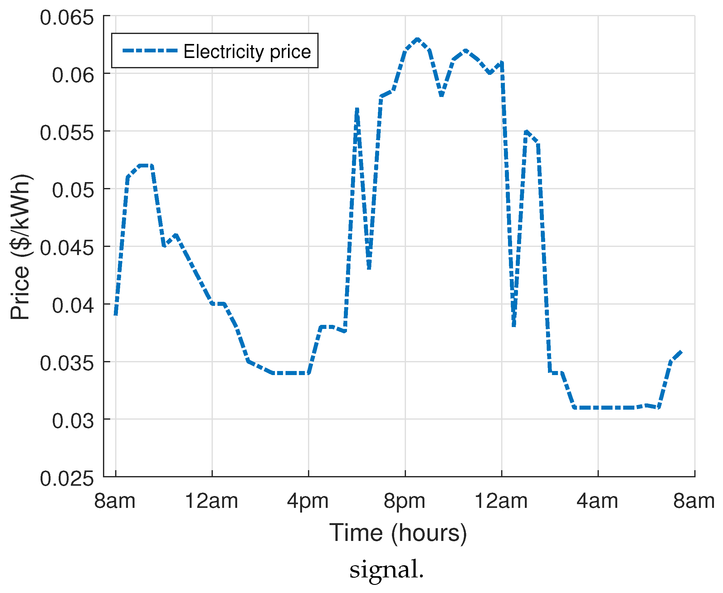
Figure 11.
Hourly electricity demand. Teaching learning-based optimization (TLBO); enhanced differential evolution (EDE); and enhanced differential teaching learning algorithm (EDTLA).
Figure 11.
Hourly electricity demand. Teaching learning-based optimization (TLBO); enhanced differential evolution (EDE); and enhanced differential teaching learning algorithm (EDTLA).
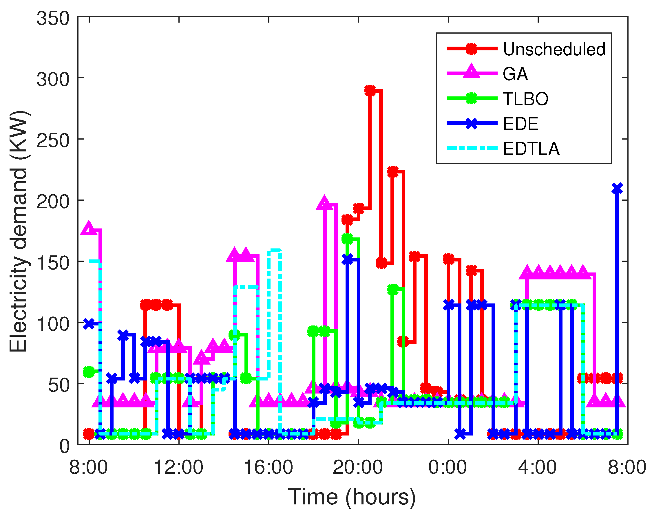
Figure 12.
Hourly electricity demand with RESs and battery storage system (BSS).
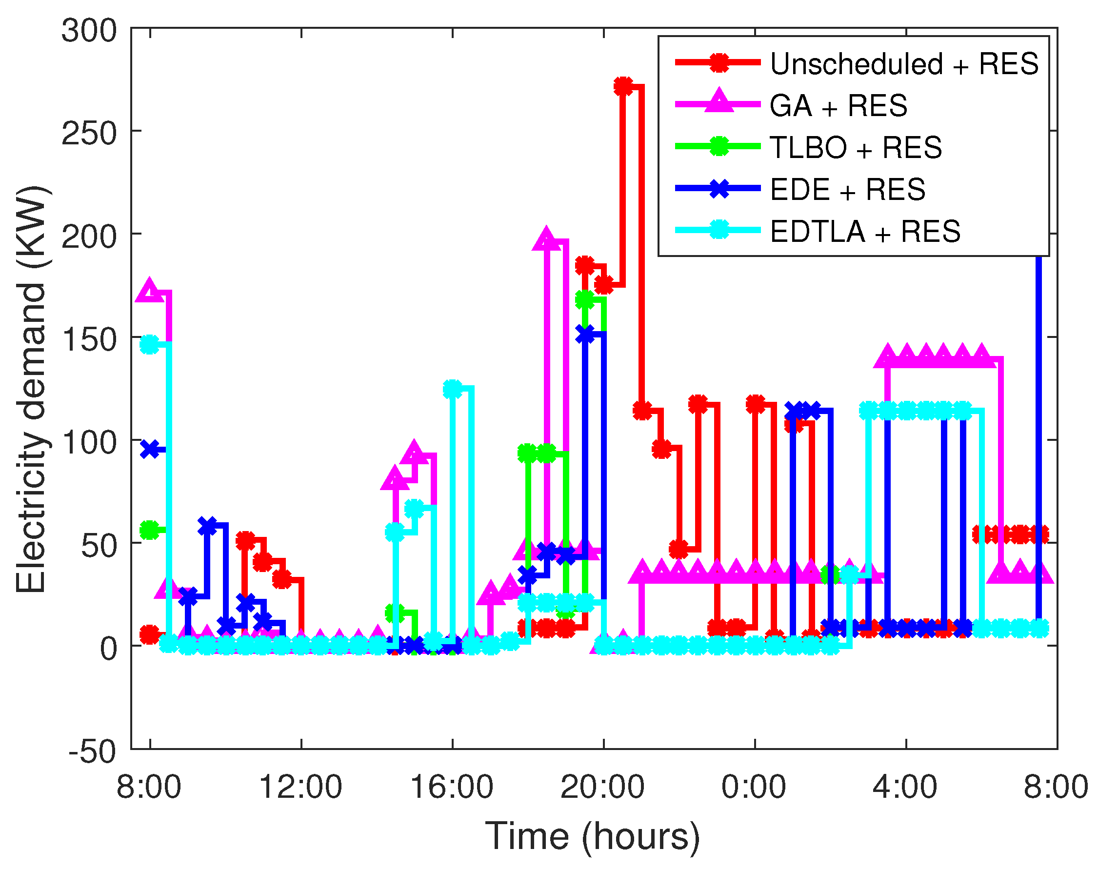
Figure 13.
Estimated energy generation.
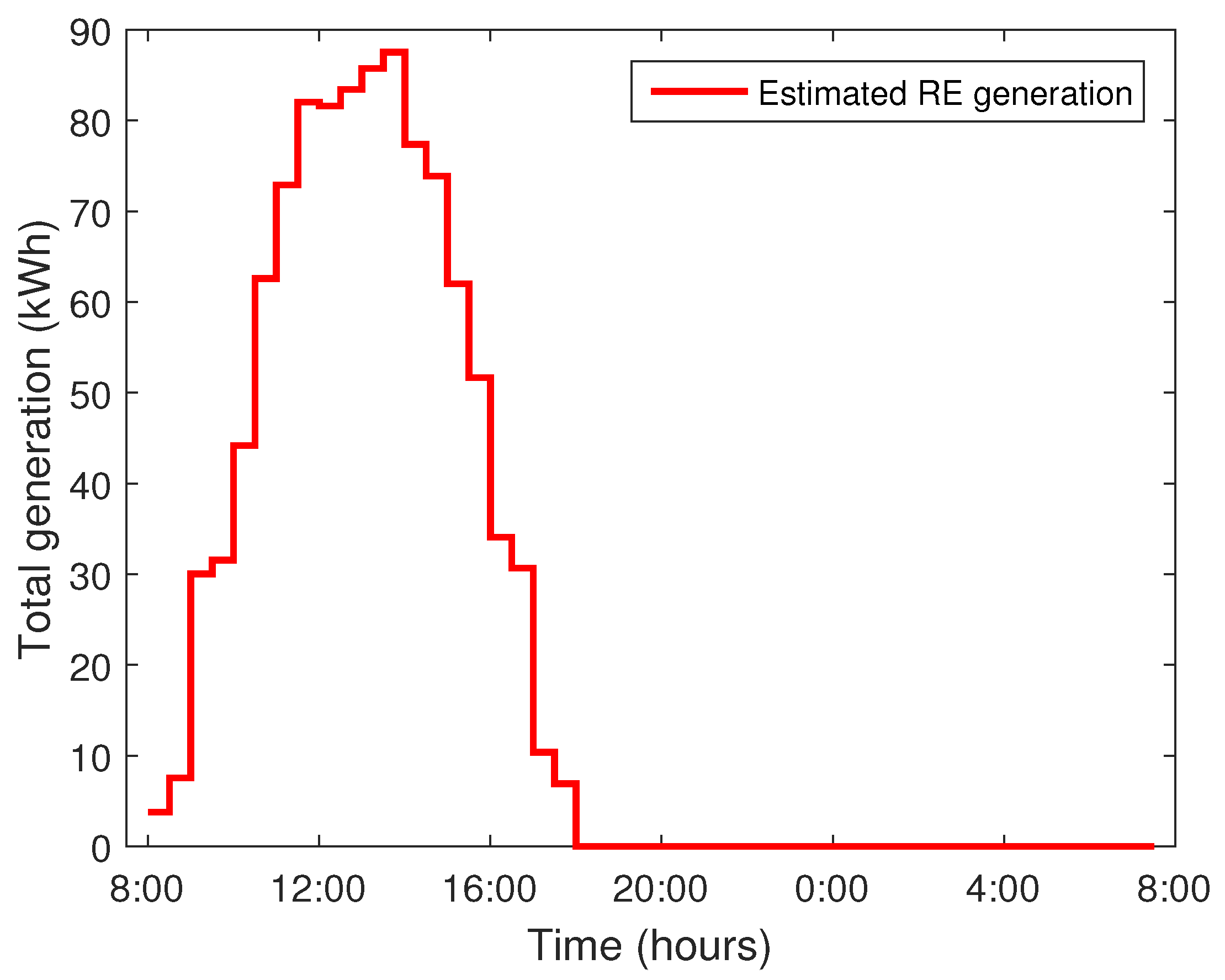
Figure 14.
Hourly electricity cost.
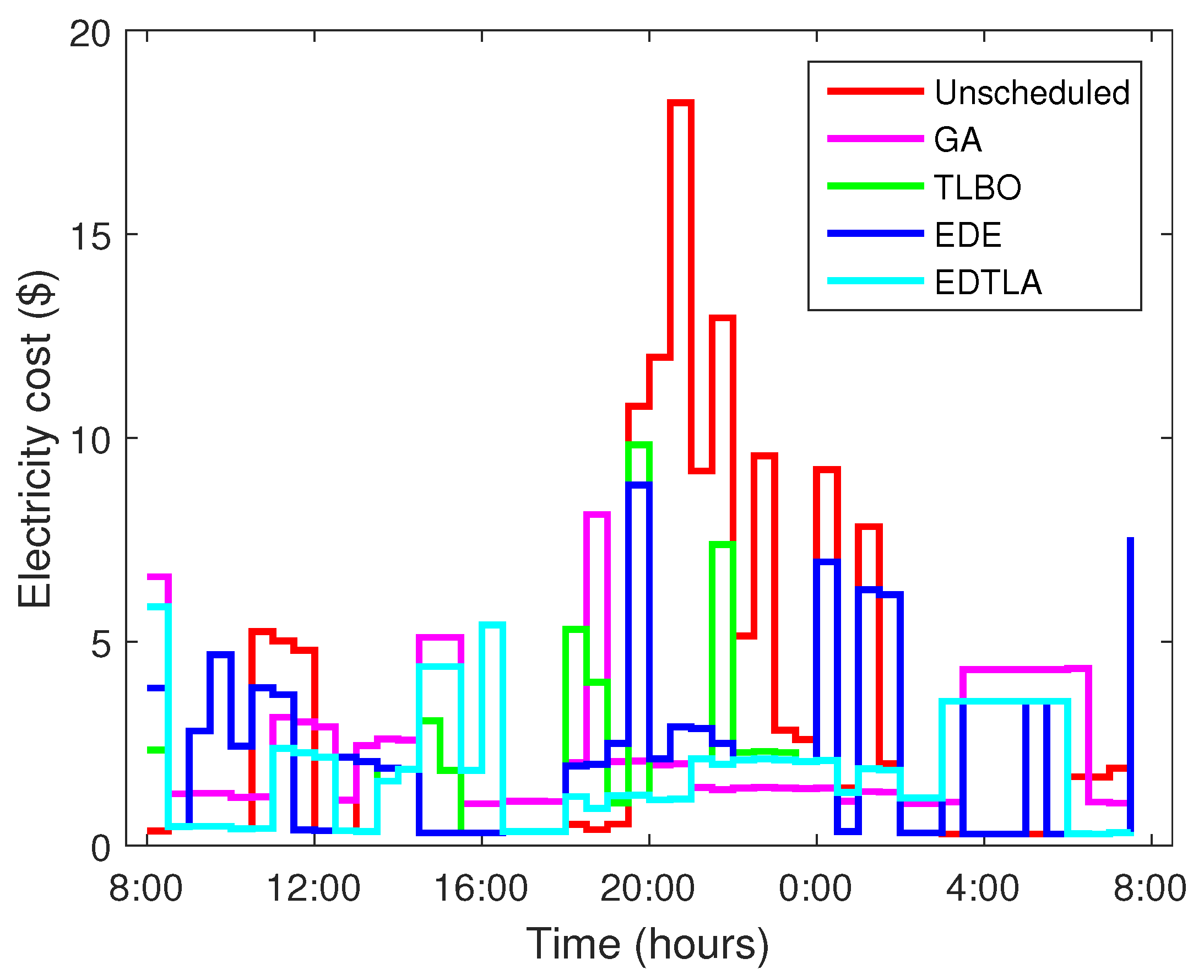
Figure 15.
Daily electricity bill.

Figure 16.
Hourly electricity bill with RESs and BSS.

Figure 17.
Daily electricity bill with RESs and BSS.

Figure 18.
Peak to average ratio (PAR).

Figure 19.
PAR with RESs integration.

Figure 20.
User discomfort.
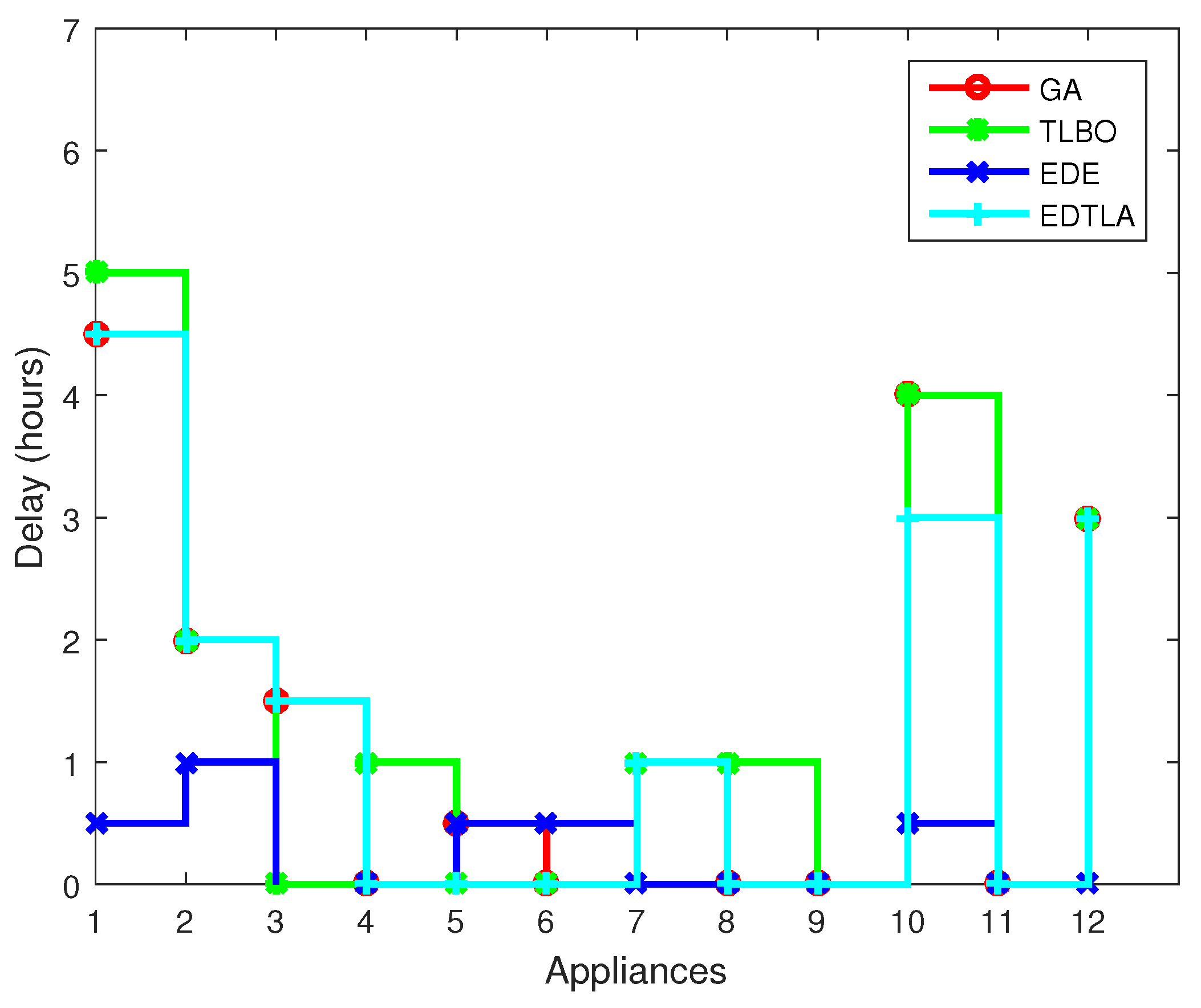
Figure 21.
Heat demand.


Table 1.
Parameters of the appliances.
| Task | Power (kW) | Earliest Starting Time (h) | Latest Finishing Time (h) | Time Window Length (h) | Duration (h) |
|---|---|---|---|---|---|
| Dish washer | 1.5 | 9 | 17 | 8 | 2 |
| Cloth washer | 1.5 | 9 | 12 | 3 | 1.5 |
| Spin dryer | 2.5 | 13 | 18 | 5 | 1 |
| Cooker hob | 3 | 8 | 9 | 0.5 | 0.5 |
| Cooker oven | 5 | 18 | 19 | 0.5 | 0.5 |
| Microwave | 1.7 | 8 | 9 | 0.5 | 0.5 |
| Lighting | 0.84 | 18 | 24 | 6 | 6 |
| Laptop | 0.1 | 18 | 24 | 6 | 2 |
| Desktop | 0.3 | 18 | 24 | 6 | 3 |
| Cleaner | 1.2 | 9 | 17 | 8 | 0.5 |
| Fridge | 0.3 | 0 | 24 | - | 24 |
| Electric car | 3.5 | 18 | 8 | 14 | 3 |
Table 2.
Technical parameters of distributed energy resources (DERs).
| Resource | Capacity | Efficiency (%) | Operation/Maintenance Cost (%) |
|---|---|---|---|
| CHP | 20 kW | 40 | 2.7 cents/kWh |
| Boiler | 120 kW | 85 | 2.7 cents/kWh |
| Storage | 10 kWh | 90 | 0.5 cents/kWh |
Table 3.
Summarized results of CO, peak to average ratio (PAR) and cost reduction.
| Technique | Total Load (kW/day) | Total Cost ($/day) | CO Emissions (kg) | PAR Reduction (%) | Cost Reduction (%) |
|---|---|---|---|---|---|
| Unscheduled | 1056 | 135.88 | 551.3 | - | - |
| GA | 1056 | 116.37 | 551.3 | 17.30 | 14.70 |
| TLBO | 1056 | 89.4784 | 551.3 | 30.76 | 33.82 |
| EDE | 1056 | 118.66 | 551.3 | 15.38 | 12.76 |
| EDTLA | 1056 | 82.14 | 551.3 | 43.61 | 36.02 |
Table 4.
Summarized results with RESs and battery storage system (BSS).
| Technique | Grid Energy (kW/day) | RESs Generation (kW/day) | Total Cost ($/day) | PAR Reduction (%) | Cost Reduction (%) | CO Reduction (%) |
|---|---|---|---|---|---|---|
| Unscheduled | 630 | 426 | 92.63 | - | - | 40.35 |
| GA | 566 | 490 | 84.2461 | 11.29 | 36.76 | 46.41 |
| TLBO | 570 | 486 | 48.1144 | 14.51 | 64.70 | 46.03 |
| EDE | 600 | 456 | 62.2162 | 11.02 | 52.94 | 56.82 |
| EDTLA | 580 | 476 | 44.8372 | 29.41 | 67.44 | 54.94 |
Table 5.
Execution time.
| Algorithm | Time (s) | Time with RES (s) |
|---|---|---|
| Unscheduled | 0.09314 | 0.195858 |
| GA | 3.4122 | 4.6754 |
| TLBO | 8.0142 | 8.2490 |
| EDE | 1.2841 | 2.4903 |
| EDTLA | 8.9164 | 9.9490 |
© 2017 by the authors. Licensee MDPI, Basel, Switzerland. This article is an open access article distributed under the terms and conditions of the Creative Commons Attribution (CC BY) license (http://creativecommons.org/licenses/by/4.0/).
Share and Cite
MDPI and ACS Style
Javaid, N.; Hussain, S.M.; Ullah, I.; Noor, M.A.; Abdul, W.; Almogren, A.; Alamri, A. Demand Side Management in Nearly Zero Energy Buildings Using Heuristic Optimizations. Energies 2017, 10, 1131. https://doi.org/10.3390/en10081131
AMA Style
Javaid N, Hussain SM, Ullah I, Noor MA, Abdul W, Almogren A, Alamri A. Demand Side Management in Nearly Zero Energy Buildings Using Heuristic Optimizations. Energies. 2017; 10(8):1131. https://doi.org/10.3390/en10081131
Chicago/Turabian StyleJavaid, Nadeem, Sardar Mehboob Hussain, Ibrar Ullah, Muhammad Asim Noor, Wadood Abdul, Ahmad Almogren, and Atif Alamri. 2017. "Demand Side Management in Nearly Zero Energy Buildings Using Heuristic Optimizations" Energies 10, no. 8: 1131. https://doi.org/10.3390/en10081131
Note that from the first issue of 2016, this journal uses article numbers instead of page numbers. See further details here.