Identification of Critical Transmission Lines in Complex Power Networks

1
Power System Protection and Control Research Laboratory, Beijing Jiaotong University, Shangyuancun No. 3, Haidian District, Beijing 100044, China
2
School of Electrical and Electronic Engineering, The University of Manchester, Manchester M13 9PL, UK
*
Author to whom correspondence should be addressed.
Energies 2017, 10(9), 1294; https://doi.org/10.3390/en10091294
Submission received: 3 August 2017
/
Revised: 25 August 2017
/
Accepted: 25 August 2017
/
Published: 30 August 2017
(This article belongs to the Section F: Electrical Engineering)
Abstract
:Growing load demands, complex operating conditions, and the increased use of intermittent renewable energy pose great challenges to power systems. Serious consequences can occur when the system suffers various disturbances or attacks, especially those that might initiate cascading failures. Accurate and rapid identification of critical transmission lines is helpful in assessing the system vulnerability. This can realize rational planning and ensure reliable security pre-warning to avoid large-scale accidents. In this study, an integrated “betweenness” based identification method is introduced, considering the line’s role in power transmission and the impact when it is removed from a power system. At the same time, the sensitive regions of each line are located by a cyclic addition algorithm (CAA), which can reduce the calculation time and improve the engineering value of the betweenness, especially in large-scale power systems. The simulation result verifies the effectiveness and the feasibility of the identification method.
1. Introduction
Due to the expansion of power grids and increases in load demand, the power systems gradually approach their operating limits. This increases the uncertainty of the system dynamic behavior and the risk of large blackouts [1]. Many power outages have occurred in recent years [2,3], for instance, the western North America blackouts in 1996 [4], the North American blackouts in 2003 [5], and the India blackouts in 2012 [6]. Frequent accidents expose the potential problems of current power system analysis methods, especially concerning system vulnerability.
In a blackout, critical lines often trigger or promote the failure propagation. These lines usually play important roles in the network structure, and their disconnections greatly increase power system vulnerability and can even cause serious consequences. Accurately identifying the critical transmission lines can realize rational planning and provide reliable security pre-warning. It also helps to ensure control measures are carried out effectively to avoid the occurrence of blackouts.
At present, researches on the identification of critical or vulnerable transmission lines are usually based on three main factors: the network topology [7,8,9,10,11,12,13,14,15,16], the electrical characteristics [17,18,19,20,21,22,23], and the failure mechanism [24,25,26,27]. Power grids can be conceptually described as networks, so that topology-based theory provides a feasible way to study network vulnerability [7] and locate the critical transmission lines [8,9]. Some indices, such as betweenness [10,11,12,13], are proposed to describe the importance of different components. In topology-based methods, the betweenness of an edge is defined as the number of the shortest paths through it. Reference [14,15,16] indicated that the nodes and lines with high betweenness and high degrees play key roles in guaranteeing the connectivity and stability of the grid. However, pure topology-based methods ignore the electrical characteristics and often cannot completely reflect the complexity of operations [17]. Some researchers try to locate important substations and lines by using the electrical parameters [18,19,20,21,22]. An electrical betweenness was proposed in Reference [19] to quantify the role of each line in the entire grid by using the sum of absolute value of power in different directions. Reference [20] improved the electrical betweenness by considering the maximal load demand and the capacity of generators in power grids. A concept of network centrality for power systems based on system responses and topological features was presented in Reference [21]. It aims to identify critical components with an equivalent electrical model. Chen et al. [22] calculated electrical efficiency based on the admittance matrix, but assumed that power was transmitted through the most effective paths. In reality, power flow is not limited to transfer along the lines with the smallest impedance, but in all possible ways. In Reference [23], a hybrid flow betweenness (HFB) based identification method was proposed. The new betweenness covers the direction of power flow, the maximum transmission capacity, the electrical coupling degree between different lines, and outage transfer distribution factor with a more comprehensible physical background. From the perspective of the development mechanism of large-scale blackouts, Reference [24] searched for sensitive transmission lines on the basis of the criticality of system cascading collapses. Wang et al. [25] used the fault chain theory to perform cascading failures initiated by faults on different transmission lines. The number of disconnected lines is basically used to derive the vulnerability index for identifying the sensitive initial lines. This type of method [24,25,26,27] is usually based on numerous simulations, and cannot reflect the actual power flow properties and operational states well.
It is reasonable to assess network vulnerability and identify critical transmission lines of power systems with electrical and topological characteristics. However, the existing methods are mainly based on the inherent parameters of the whole power system, without enough ability to take real-time data into account. In this study, a new integrated betweenness is proposed to comprehensively consider the function of a line and the impact when it is removed from a power system. Compared with previous studies, the betweenness evaluates the role of the transmission line from the perspective of the power transmission distance, improves the impact analysis of fault flow distribution, and considers the system security with the tolerance of the remaining network. At the same time, a new searching algorithm, named cyclic addition algorithm (CAA), is proposed to locate the sensitive regions that are significantly affected by a removed line. Thus the calculation time of the betweenness can be reduced and the new identification method is more valuable in engineering applications.
The rest of the paper is structured as follows: Section 2 introduces the definition and the calculation method of the integrated betweenness of a transmission line, which consists of the indices of the power transmission, the fault flow distribution, and the influence on system security. Section 3 presents the detailed identification process with integrated betweenness and CAA. The simulation results with the IEEE 39-bus system are provided in Section 4, which prove the accuracy and effectiveness of the identification method. Finally, conclusions are given in Section 5.
2. Integrated Betweenness to Identify Critical Lines
“Vulnerability” or its opposite concept “robustness” is often used to evaluate the ability of a power grid to provide key services or functions in normal operations, with random failures or under intentional attacks [18]. A critical transmission line plays an important role in maintaining the security and stability of the power system. When it is removed due to external attacks or its own failure, the system may suffer from a serious impact, and even have a high probability of cascading trips. Therefore, the integrated betweenness proposed in this study comprehensively considers the role of a transmission line in a power system, the redistribution of power flow caused by a fault on the line, and the corresponding influence on system security.
Taking line i as an example, Di, Hi and Ci are respectively the indices of the power transmission, the fault flow distribution, and the influence on system security. The integrated betweenness Wi of line i can be calculated by:
where Di′, Hi′, and Ci′ are normalized absolute values of Di, Hi, and Ci, as can be obtained by a linear normalization method. The values of Di′, Hi′ and Ci′ are all between 0 and 1. Di is the index of power transmission, and is used to reflect the role of line i in the power transmission network. It can be calculated by the difference of the transmission distances of the whole power grid with and without line i. DP0 is the transmission distance of active power in the grid inclusive of line i, while DPi is the transmission distance after the removal of line i; Hi is the index of fault flow distribution. It reflects the impact caused by a fault on line i. Hi can be obtained by the ratio of the amount and the distribution entropy Bi of transferred power. Zim is the power change on line m when a fault happens on line i. Ψ is the set of lines with increased power. The greater the transferred power is, the larger the impacts on the other lines are. The smaller the distribution entropy Bi is, the more concentrated the power flow transfer is. A substantial increase in the transmission power can bring about harmful effects, such as the exposure of hidden failures. Ci is the index of influence on system security. Ciψ and Cimax are respectively the global and the maximum influence considering the tolerance of the remaining network. The calculation method of Di, Hi, and Ci is described in Section 2.1, Section 2.2 and Section 2.3.
2.1. The Index of Power Transmission
The importance of a line depends on its role in power transmission. The transmission distance of active power is defined as:
where xl is the electrical length of line l. It can be expressed by the reactance value, xl = xab, where xab is the element at row a and column b in the reactance matrix of a power grid; a and b are the two ends of line l; pl(g, d) is the active power on line l when power is transmitted from generator node g to load node d; G is the set of generators, L is the set of loads and T is the set of lines.
The above equation can be simplified to:
where pl is the total active power on line l, as calculated by a DC power flow model [28]:
where θ(a) and θ(b) are the phase angles of a and b. The index of power transmission of line i is [29]:
where DP0 and DPi are the transmission distances with and without transmission line i. Di can express the change of the transmission distance of active power directly. From Equations (3)–(5), Di can be expressed as:
where ∆θl is the phase difference of the two ends of line l; T0 and Ti are the sets of lines in the system before and after the removal of line i. Based on DC power flow model, ∆θ can be calculated by:
where ∆θ is the matrix of phase difference; A is the node-branch incident matrix; B is the electrical susceptance matrix; and, Ping is the vector of injected power. Equation (7) can be used to calculate ∆θ0 and ∆θi, the matrixes of transmission distances with and without line i. Equation (5) can then be expressed as:
where r0 and ri are the numbers of lines in the system before and after the removal of line i; ∆θ0a and ∆θia are the elements at row a in matrix ∆θ0 and ∆θi.
2.2. The Index of Fault Flow Distribution
Fim(g, d) is defined as the change of power on line m, as related to the power transferred from generator g to load d, when a fault happens on line i. It can reflect the impact on line m caused by the removal of faulty line i. Fim(g, d) can be calculated by the line outage distribution factor (LODF) [30]:
where LODFim(g, d) is the power increment of line m when unit power is transferred between generator g and load d, and a fault happens on line i; Pgd is the power flow from generator g to load d, as calculated by the power flow tracing method [31].
Considering the reverse overload, the change of power can be calculated as:
where P0m(g, d) is the power flow on line m in normal operating condition, and Zim is the change of power on line m when line i is disconnected. In the DC power flow model, Zim can also be obtained using the calculation result of Equation (4). For the lines with increased power, the sharing ratio of power flow transfer on each line is:
where δim is the sharing ratio of line m when line i is disconnected; Ψ is the set of lines with increased power. The entropy of the fault flow distribution is:
The entropy Bi is used to describe the distribution of Zin, n = 1, 2, 3, …, m, … When the power is uniformly distributed, each component will shoulder the burden equally. The sharing ratio of each path is δ = 1/N, where N is the number of transferable paths. Bi is the maximum, as is lnN. Similarly, the smaller the value of Bi is, the more concentrated the transferred power flow is [32]. It means that the disconnection of line i will have significant influence on a few lines, which may overload these lines and even trigger a cascading failure. Thus, the index Hi can be used to show the distribution of fault flow, i.e.,
2.3. The Index of Influence on System Security
Although the disconnections of some lines can cause a significant transfer of power flow, detrimental consequences may not be caused if other lines have large capacities and can successfully share the transferred power. Sometimes, the influence is not great, but the operating condition is close to the safety limits, and the disconnection of a line may force the system into a dangerous operating condition. Hence it is important to consider the redistribution of power flow and the tolerance of the remaining network when evaluating the importance of a line in the whole system. In this paper, the global influence and the influence on each line caused by the removal of line i are analyzed. The index of the influence on line m is:
where Sm is the remaining available channel of line m before the removal of line i. The global influence can by calculated by:
where r0 is the number of lines in the power system, and CiΨ is the average value of Cim. The influence on system security is:
where Cimax is the maximum value of Cim, and Ci is the average value of the global influence and the maximal influence.
2.4. The Threshold of the Integrated Betweenness
If the removal of line i causes the overload of any other line in the power grid, line i can be considered a critical component [33]. In order to better assess whether the line is critical, three thresholds Dth, Hth and Cth are defined next:
(1) Dth:
where xa is the electrical length of line a; pcpa is the remaining available channel of line a; xb is the electrical length of line b; pb is the total active power on line b; and, T0 is the set of lines in the power system. For line i, Di = DPi − DP0 and DPi has already subtracted , so min is also subtracted from Dth.
(2) Hth: Hi can reflect the impact caused by a fault on line i. To avoid missing critical lines, Hth should be the minimum Hi when one remaining line is overloaded after the fault. To get the minimum Hi, the entropy Bi of the fault flow distribution should be as large as possible and in Equation (13) should be as small as possible. Let us assume the smallest remaining available channel of a transmission line is pmincp, and pmincp = minpcpa, a T0. Bi takes the maximum value, i.e., ln(r0 − 1), and takes pmincp ignoring the complex conditions. The threshold of H is:
(3) Cth: When only one remaining line is overloaded and other lines are not affected, Cimax = 1 and Ciψ =1/(r0 − 1). The threshold of C is:
Wth equals to the sum of normalized Dth, Hth and Cth, i.e.,
where Dth′, Hth′ and Cth′ are normalized absolute values of Dth, Hth and Cth. The transmission line, the integrated betweenness of which is greater than Wth, can be regarded as a critical component. The mathematical formulae for Dth, Hth, and Cth give out small values. Such small threshold values prevent missing the detection of critical lines. After the above process, these lines can be sorted according to W.
3. Identification Process with Integrated Betweenness and CAA
The integrated betweenness of each line is affected by the changes in the grid’s structure or the operating mode. The calculation time is large when the approach is applied to the data of the whole power network. In fact, Di, Hi, and Ci are all related to the changes of power flow before and after line i is removed, where the changes mainly occur on particularly sensitive lines. Therefore, a cyclic addition algorithm (CAA) is proposed to locate the sensitive regions which consist of the transmission lines with large variations of power. The impact on the sensitive regions is analyzed rather than the impact on the whole power network. Thus, the calculation time of the betweenness can be significantly reduced and the proposed identification method is more suited to the real-time analysis.
The process to identify the critical transmission lines is shown in Figure 1. First, the basic data of the grid, such as the structural parameters and the information of power flow, are obtained. The data can be collected by phasor measurement units (PMUs). When the network structure or operating mode changes, the identification process of critical lines in this state will start. Possible changes of the network structure or operating mode include the disconnection/failure of primary equipment (generators, transformers, or lines), the connection/reconnection of primary equipment, and significant redistribution of power flow within the grid. Such changes can be caused by (1) faults, e.g., line trip, generator trip, and line failure; (2) planned adjustments, e.g., the operation of new generators/lines and planned load shedding. Then Wth and the integrated betweenness of each line are calculated: sensitive regions can be located by CAA, and the remaining regions are regarded as non-sensitive regions in this study. Since the influence of the non-sensitive regions on the calculation results is quite small, those regions can be simplified as sources and loads. The number of lines and substations in the system is greatly reduced after the simplification, so that the integrated betweenness W can be calculated more quickly. With the calculation method introduced in Section 2, W of each line can be obtained. Finally, the critical lines can be identified.
Location of Sensitive Regions with CAA
The power flow is transferred on all feasible paths, but the transferred power on each path is quite different. As can be seen from previous studies [26,27,28,29,30,31], when a transmission line is disconnected or removed from the power network, the power is usually transferred to other paths connected with the two-end nodes of the removed line, and mainly along the paths with short electrical distances, as is shown in Figure 2.
The topological analysis-based method can provide a quick and effective way to identify the network structure and find propagation paths of power flow transfer [34]. Some new approaches, such as the compressive sensing-based approach [35] and graphical learning-based approach [36,37] were proposed in recent years. Based on Dijkstra’s algorithm [38], CAA is proposed in this study. The sensitive regions can be obtained through the cyclic addition of different lines. The following is a detailed description of the process.
Supposing there are a substations and b lines, all substations in the power grid can be simplified as nodes and form V according to graph theory, as is V = {v1, v2, ..., va}. All lines are represented by the edge set E, E = {e1, e2, e3, …, eb}. V and E constitute G(V, E), the topology graph of the power grid. All different paths connecting vi and vj in graph G form set D(G, vi, vj), and the length of path d is l(d). The line reactance is used as the weight of an edge, and l(d) is the sum of the weights of all edges in path d.
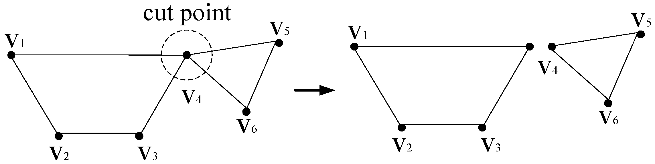
Theoretical principle 1: According to graph theory, if G cannot be fully connected when node v is removed, v is called the cut point in G, such as point v4 in Figure 3. Any edge and the paths connected with its two ends can only exist in the same part divided by cut points.
Theoretical principle 2: According to the conclusion in Reference [39], any path between two nodes in graph G(V, E) must be the shortest path between the same nodes in Gg (Vg, Eg), where Gg is a sub-graph of G with a few (including b) edges. It can be described as:
where dshortest (Gg, vp, vq) is the shortest path between vp and vq in graph Gg. Therefore, the path between two nodes in G(V, E) can be transformed into the shortest path between the same nodes in a sub-graph.
In this study, line e0 is defined as the removed line, while vp and vq are its two-end nodes. Vector L is built to store the shortest distance between any two nodes which has been found currently. For the graph with a nodes, there are Ca2 elements in L and the elements can be described as L(1–2), L(1–3), L(1–4), …, L(1–a), L(2–3), L(2–4), …, L((a − 1)–a), where L(i–j) is the shortest distance between vi and vj, and i and j can be interchanged. Vector HJ is built to store the successor nodes along the shortest path. Similarly, there are Ca2 elements in HJ and the elements can be described as HJ(1–2), HJ(1–3), HJ(1–4), …, HJ(1–n), HJ(2–3), HJ(2–4), …, HJ((a − 1)–a). Each sub-graph has corresponding values for L and HJ.
Step 1: Find cut points and divide the graph into different parts. Find the parts G’ where e0 is located. Suppose that there are m lines and n nodes in G’. Delete e0 and get all the other edges in graph G’. Let k = 1.
Step 2: Select k edges, and there are Cm−1k different selection results. Let c = 1.
Step 3: Deal with the selection result c, where k edges and their connected nodes constitute a sub-graph G’kc. If vp or vq is an isolated node without any connected lines, or vp and vq are located in different islands in G′kc, go to step 8, i.e., the sub-graph can be ignored directly; otherwise go to step 4.
Step 4: Take away and rank k edges. Let f = 1 and initialize Lkc and HJkc. When there is no edge in graph G’kc, the values of the elements in Lkc are equal to an infinite value, as is Lkc = [∞, ∞, ∞, …, ∞]. All elements in HJkc are Ø, showing there is no path currently.
Step 5: Put edge f back. The two-end nodes of f are vu and vv, vu and vv V′kc. Next apply the following judgment: If Lkc(u − v) < l(f), go directly to step 7. Otherwise, let Lkc(u − v) = l(f), HJkc(u − v) = v, and go to step 6.
Step 6: Deal with Lkc and HJkc:
For w (1 ≦ w ≦ n, w ≠ u, w ≠ v):
If Lkc(u − w) > Lkc(u − v) + Lkc(v − w), change the value of Lkc(u − w) into Lkc(u − v) + Lkc(v − w), and change HJkc(u − w) into v; If Lkc(v − w) > Lkc(u − v) + Lkc(u − w), change the value of Lkc(v − w) into Lkc(u − v) + Lkc(u − w), and change HJkc(v − w) into u;
If Lkc(u − w) = Lkc(u − v) + Lkc(v − w) ≠ ∞, insert v into HJkc(u − w); If Lkc(v − w) = Lkc(u − v) + Lkc(u − w) ≠ ∞, insert u into HJkc(v − w); then go to step 7.
Step 7: If f = k, go to step 8; otherwise f = f + 1, then go back to step 5.
Step 8: If c = Cm−1k, go to step 9; otherwise c = c + 1, then go back to step 3.
Step 9: if k = m−1, go to step 10; otherwise k = k + 1, then go back to step 2.
Step 10: All the paths between vp and vq and their lengths can be got. Remove duplicate paths.
Supposing that there are y paths between vp and vq, the lengths of all paths (l(1), l(2), ..., l(y)) can be derived by the above process. According to the principle of electric circuits, the transferred power flow on path d changes inversely with the length l(d). Thus, the power sharing coefficient of edge i is:
where μ is the set of paths which contain line i. Judge whether the power sharing coefficient can satisfy:
where ξth is the threshold value, ξth ≥ 0. If (23) is satisfied, line i will be regarded as a sensitive line, as is closely related to line e0. The sensitive lines should be selected effectively and the sensitive regions which consist of sensitive lines should be fully connected. According to the definition of sensitive lines or transmission sections in Reference [40], the threshold value usually varies between 0.2 and 0.3. Based on the above analysis, the threshold ξth can be obtained by the following iterative process: ξth is initialized with 0.3. If the sensitive regions are not fully connected, ξth will be decreased with a fixed step size, until the requirement of full connection can be satisfied or the value of ξth is 0.
To improve the accuracy of integrated betweenness and to avoid missing sensitive lines, ξth can be taken as 0 directly in an extreme situation.
Sensitive regions can be obtained by the above process. For G′ with m lines and n nodes, the calculation amount of the cyclic process in CAA in the worst condition is:
where P = 1 means that one element in L or HJ is updated once. For G′ with m lines and n nodes. Cm−1k is the number of sub-graphs with k lines. In the worst case, all sub-graphs can satisfy the requirement in step 3, and none will be ignored. 2(n − 2) + 1 elements in L and 2(n − 2) + 1 elements in HJ are updated when one transmission line is put back through steps 5 and 6. The process of CAA only contains some simple comparisons based on a pure topology model. Therefore, the calculation time of the identification method can be significantly reduced. At the same time, it should be noticed that CAA is effective for most lines in power systems. For the lines which do not have other paths connected with their two ends, the removal of the lines can result in the islanding phenomenon. In these cases, the injected power of sources and absorbed power of loads in each island should be balanced first. After that, the calculation of the integrated betweenness can be carried out using the analysis of the whole power network.
4. Test Cases
In this section, IEEE 39-bus system is used as the test system to demonstrate the effectiveness of the proposed method.
4.1. Location of Sensitive Regions
4.1.1. Location of Sensitive Regions with CAA
Line e33 is taken as an example and used to show the detailed process to locate the sensitive regions.
Firstly, all substations and lines are simplified as nodes and edges. Line e33 is the removed line, while v26 and v29 are its two-end nodes. Divide the graph into different parts with cut points v26 and v16 in Figure 4. G’ which contains v26, v28, v29, e32, e33 and e34 is found, and then e33 is deleted. The edges e32 and e33 in graph G’ are taken away. Let k = 1. Select 1 edge, and it can be seen that there is no path between v26 and v29 in all the sub-graphs with one edge and two nodes. Let k = 2. Taking sub-graph G’21 as an example, the sub-graph is shown in Figure 5. Since the topology of G′21 is simple, the power sharing coefficient of each edge can be obtained directly. To better illustrate the application of CAA, the calculation process is introduced in detail.
With the analysis of step 3, the sub-graph is kept. Take away and rank the 2 edges. Let f = 1, and initialize L21 and HJ21. The elements in L21 are [L21(26–28), L21(26–29), L21(28–29)]. The elements in HJ21 are [HJ21(26–28), HJ21(26–29), HJ21(28–29)]. L21 = [∞, ∞, ∞] and HJ21 = [Ø, Ø, Ø].
Put edge e34 back. The weight of the edge l(e34) is 0.0151, which is smaller than L21(28–29). Therefore, let L21(28–29) = 0.0151. After the step 5, L21 = [∞, ∞, 0.0151] and HJ21 = [Ø, Ø, 29]. Because L21(26–28) = L21(28–29) + L21(26–29) = ∞ and L21(26–29) = L21(28–29) + L21(26–28) = ∞, do nothing to L21 and HJ21 according to step 6. Go to step 7, i.e., f = f + 1 = 2. Then go back to step 5.
Similarly, put edge e32 back. L21 = [0.0474, 0.0625, 0.0151] and HJ21 = [28, 28, 29].
The length of the shortest path between nodes v26 and v29 in graph G′21 is 0.0625 according to L21(26–29). The successor node of v26 is v28, and the successor node of v28 is v29, which can be got by HJ21(26–29) and HJ21(28–29). Then the shortest path v26–v28–v29 can be obtained. The power sharing coefficients of e32 and e34 are 1. ξth is set to 0.3. The sensitive region, which includes line e32 and e34 is now derived.
By two simple comparisons, the analysis of all lines in the whole network can be simplified as the analysis of two lines. The order of the matrixes, such as A and B in Equation (7), can be reduced from 39 to 3 during the calculation of the integrated betweenness.
4.1.2. Comparison of CAA and Depth-First-Search Method
For the purpose of comparing the performance of CAA and Depth-First-Search (DFS) [41] algorithm, line e33 is used as an example. Both algorithms are used separately to find the paths from v26 to v29 after line e33 is removed.
The CAA proposed in the study uses the topological method to search for all possible paths connecting the two-end nodes of the removed line and obtain the power sharing coefficients of different edges. The DFS algorithm explores a graph by starting at a node and going as deep as possible. Such DFS traversal is a type of backtracking method, and therefore exhibits poor performance.
With CAA, the relevant sub-graph can be located at first, which effectively cleans up all useless edges and reduces the search scope. Then, the path and its length can be obtained directly after two comparisons. With DFS, v26 is set as the starting node. v25, v27 and v28 can be reached in the next step. The paths through v25 or v27 are not feasible by several explorations and backtracking. The only feasible path is v26–v28–v29.
As can be seen from Section 4.1.1 and the above analysis, the proposed CAA can delete useless lines and sub-graphs to avoid invalid search directions. In this case, the search results with CAA and DFS are identical, but the computation time with CAA is 78.6% shorter than that with DFS.
4.1.3. Accuracy Analysis of the Location Method
(1) To show the validity of the location method, branch e33 is removed at 0.5 s. The simulation result based on PSASP is shown in Table 1. As can be seen from the simulation results, there is a large increase in the power transferred on the transmission lines in the sensitive regions, while the increases on un-sensitive lines are much smaller.
(2) Line e20 is removed at 0.2 s. The simulation result is shown in Table 2. When ξth is 0.3, there are e4, e5, e6, e8, e12, e16, e17, e18, e19, e21, e25, e26, e30, and e31 in sensitive regions. The first 14 branches with large power variations are included.
4.2. Analysis of Identification Results
4.2.1. Identification Result with Integrated Betweenness and CAA
ξth is set as 0 to insure the accuracy of the identification. The capacity of each line is 5 times the initial active power. The sensitive regions can be located by CAA, and the non-sensitive regions are simplified as sources and loads. Based on that, the integrated betweenness of each line can be calculated. For the lines whose removal can result in islanding phenomenon, the injected power of sources and the absorbed power of loads in each island should be balanced. In this study, the absorbed power of each load and the injected power of each source are reduced in proportion to their initial power and according to the minimum load shedding method as described in Reference [42].
During the identification process, the shortest computation time of W for a single transmission line is 0.515 ms, and the longest time for a single line is 8.416 ms. The computation time of the whole process is 0.061 s. Without CAA, the computation time is 0.286 s when the approach is applied to the data of the whole power network. The results prove that the CAA is effective in reducing the computation time.
The final results of the indices and the betweenness are shown in Table 3. Wth = 0.2546. e6, e14, e15, e19, e24, e26, and e28 cannot be regarded as critical lines. Compared with the results calculated by the global network, the average error rate of index H with the data of sensitive regions is 2.8%, and the average error rate of index C is 1.02%. The average error rate of integrated betweenness W is 2.24%. The accurate identification result can still be obtained through the process of simplification.
4.2.2. Comparison of Lines with Different Integrated Betweenness
Taking lines e27, e20 and e29 as examples, the increased power of transmission lines at 1 s in IEEE 39-bus system is shown in Figure 6, when e27, e20 and e29 are removed individually at 0.5 s.
It can be seen clearly from Figure 6a that the total amount of power flow transfer is quite large and it is mainly concentrated on lines e24, e28, and e29 when line e27 is removed. It means that the disconnection of line e27 has significant influence on the power system. The comparison of Figure 6b,c shows that the transferred power is more concentrated when line e29 is removed. But the total transferred power and the global impact is less compared with the removal of line e20. The above phenomena are consistent with the values of D, H, and C, which proves the validity and rationality of the indices.
4.3. Comparison of Identification Results
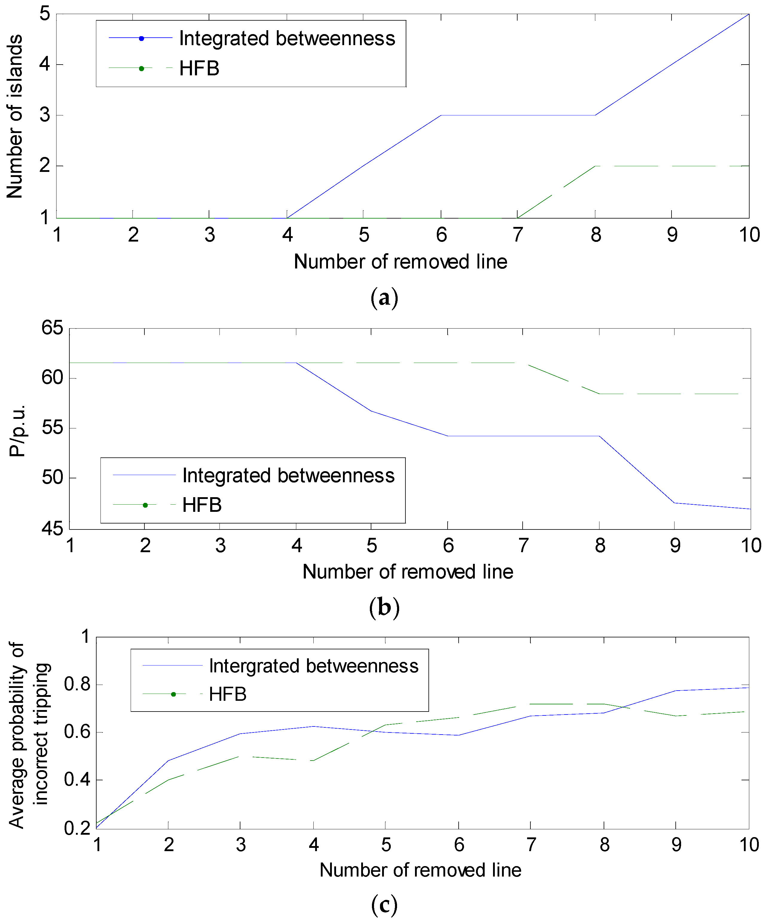
To verify the effectiveness of the identification method with integrated betweenness, the top 10 lines are attacked. When compared with the attacks performed according to the hybrid flow betweenness (HFB) as introduced in Reference [23], the number of islands, the total value of the loads, and the average vulnerability of the remaining network are shown in Figure 7. The loss of loads can be determined according to the minimum load shedding method [42]. The average vulnerability of the transmission lines is evaluated using the probability of incorrect tripping caused by the current increment. The linear function of the probability can be obtained according to Reference [43]. In this study, the probability of incorrect tripping is set to 0 when there is no current increment on the transmission line, and the probability is set to 1 when the current is greater than 1.4 times the rated value.
On the basis of the direction and distribution of power flow, HFB considers the electrical coupling between the lines and the influence caused by a single line fault. Compared with HFB, the integrated betweenness proposed in this study improves the impact analysis of fault flow distribution and considers the tolerance of the remaining network. The top 10 lines are e27, e3, e20, e31, e4, e23, e34, e12, e21, and e29 according to the proposed integrated betweenness and e11, e20, e3, e16, e29, e12, e1, e19, e7, and e5 as according to the HFB. The lines are attacked and disconnected in turn, and the impact of each disconnection on the remaining transmission lines is analyzed.
(1) Integrated betweenness attack
According to the identification results of the proposed method, line e27 with high D, H and C will be disconnected first. The current increments on lines e24, e28 and e29 are 5.268 p.u., 5.8586 p.u. and 5.4645 p.u. These lines exhibit high current increments and will therefore have a high risk of tripping. Then, line e3 is disconnected. It will have impact on several transmission lines, namely e1, e2, e6, e7, e14, e15, e25, e30, and e31. At the same time, the current on e24, e28, and e29 continues to rise and the system risk will be further increased. Following the disconnections of lines e20 and e31, the power flow is redistributed to lines e4, e5, e17, e18, and e19.
Islanding phenomenon occurs when e4 is disconnected. The network is split into a 6-node isolated island and a 33-node system. Although the network is forced to be divided into two parts, the total amount of loads is reduced during the balance of the injected power of sources, and the absorbed power of loads in each island. Therefore, the pressure on the transmission system and the overloads of e1, e2, e7, e14, e15, e17, e18, e19, and e30 are relieved. Subsequently, e23 is disconnected. The node v21 is separated from the network, and the current on e24, e28, and e29 is slightly decreased. After the attacks on e34, e12, e21, and e29, some nodes fall off, but the average vulnerability of the remaining lines keeps increasing.
(2) HFB attack
When line e11 is disconnected, e9, e10, e14, and e15 will have a high risk of tripping. Then e20, e3, e16, e29, e12, and e1 are attacked one by one. Some transmission lines, such as e2, e6, e17, e18, e19, e21, e25, e26, and e30, are affected by the power flow transfer. Most of the current increments on these lines are between 0.2 and 0.3 p.u. and the maximum current increment is 4.4196 p.u. Subsequently, line e19 is disconnected and the node v15 is isolated from the network. Finally, e7 and e5 are attacked and the average probability of incorrect tripping is approximately 0.7.
It can be seen from Figure 7 that the islanding phenomenon is more obvious and the loss of loads is greater under the integrated betweenness attack performed on the IEEE 39-bus system. The lines with high betweenness play critical roles in the power grid. When nearly 30% of the lines are removed under integrated betweenness attack, the loss of load remains at 24%, and the vulnerability of the remaining network is also greatly improved.
4.4. Extreme Cases and Real-Time Behavior
4.4.1. Extreme Cases
IEEE 39-bus system is used as the test system in this section. The injected and absorbed power is changed to present some extreme cases.
(1) All the injected power of generators and the absorbed power of loads are reduced to 0.05 times the initial value. The calculation result is shown in Table 4. Based on the identification method, Wth = 2.3149, and no line is selected to be a critical transmission line.
(2) All of the injected power of generators and the absorbed power of loads are increased 4.99 times in respect to their initial values, to bring the system close to its stability limit. The disconnection of any line will result in a serious consequence. In this case, Wth = 0.00822. The calculation result is shown in Table 5. All lines are regarded as critical transmission lines.
4.4.2. Real-Time Behavior of Power Grids with Different Scales
The computation times of test systems with various scales are statistically analyzed. The systems include IEEE 39-bus system, IEEE118-bus system, and several large-scale systems, which are randomly synthesized by IEEE standard 30-bus and 118-bus system [44]. The standard systems are connected with high-tension transmission lines. Each system is calculated ten times. The average computation time of each test system is shown in Table 6.
Based on the above data, the computation time can be qualitatively analyzed: the computation time of the system with 39–5000 buses can be of the order of seconds, and the computation time of the system with 5000–10,000+ buses can be of the order of minutes.
The implementation of “real-time identification of critical lines” depends on two important parts: (1) measurement data acquisition; (2) data processing and analysis. The measurement data can be obtained by wide area measurement system (WAMS). According to Reference [45], WAMS is required to complete the measurement and transmission of PMU data in 30–50 ms for dynamic monitoring and real-time decision-making purposes. Based on the data in Table 6, the time scale of the identification process can be of the order of minutes.
5. Conclusions
In order to implement accurate and fast identification of critical lines, an integrated betweenness is proposed which considers the topological and electrical characteristics of the power network. The indices of power transmission, fault flow distribution, and the influence on system security are used to assess the importance of different lines with respect to the functionality of themselves, relevance with other transmission lines, and system security. Although the three indices are different, they are all related to the changes in the power system before and after the removal of a line. Based on this, the sensitive regions containing lines with large variations of power are located by CAA. The analysis of the whole network is replaced by the analysis of sensitive regions, which reduces the calculation time effectively and provides the possibility for real-time analysis in large-scale power systems.
This study focuses on the identification of critical lines which play important roles in power transmission and whose disconnections have a great influence on system vulnerability. Together with the transmission lines which are heavily overloaded or have high risks of failures, the identification results can help formulate plans to avoid blackouts. The simulation results show that the proposed method is effective and practical.
Acknowledgments
This work was supported by the National Key R&D Program of China (2016YFB0900600) and the Fundamental Research Funds for the Central Universities (NO.2017YJS178).
Author Contributions
All authors contributed to the research in the paper. The work was carried out by Ziqi Wang and performed under the advisement from Jinghan He, Alexandru Nechifor, Dahai Zhang and Peter Crossley.
Conflicts of Interest
The authors declare no conflict of interest.
References
- Hong, S.; Cheng, H.; Zeng, P. An n–k analytic method of composite generation and transmission with interval load. Energies 2017, 10, 168. [Google Scholar] [CrossRef]
- Cai, Y.; Li, Y.; Cao, Y.; Li, W.; Zeng, X. Modeling and impact analysis of interdependent characteristics on cascading failures in smart grids. Int. J. Electr. Power Energy Syst. 2017, 89, 106–114. [Google Scholar] [CrossRef]
- Zeng, K.; Wen, J.; Ma, L.; Cheng, S.; Lu, E.; Wang, N. Fast cut back thermal power plant load rejection and black start field test analysis. Energies 2014, 7, 2740–2760. [Google Scholar] [CrossRef]
- Kosterev, D.N.; Taylor, C.W.; Mittelstadt, W.A. Model validation for the 10 August 1996 WSCC system outage. IEEE Trans. Power Syst. 1999, 14, 967–979. [Google Scholar] [CrossRef]
- Piacenza, J.R.; Proper, S.; Bozorgirad, M.A.; Hoyle, C.; Tumer, I.Y. Robust topology design of complex infrastructure systems. ASCE-ASME J. Risk Uncertain. Eng. Syst. Part B Mech. Eng. 1999, 14, 967–979. [Google Scholar]
- Rampurkar, V.; Pentayya, P.; Mangalvedekar, H.A.; Kazi, F. Cascading failure analysis for Indian power grid. IEEE Trans. Smart Grid 2016, 7, 1951–1960. [Google Scholar] [CrossRef]
- Gao, J.; Liu, X.; Li, D.; Havlin, S. Recent progress on the resilience of complex networks. Energies 2015, 8, 12187–12210. [Google Scholar] [CrossRef]
- Gallos, L.K.; Cohen, R.; Argyrakis, P.; Bunde, A.; Havlin, S. Stability and topology of scale-free networks under attack and defense strategies. Phys. Rev. Lett. 2005, 94, 188701. [Google Scholar] [CrossRef] [PubMed]
- Schneider, C.M.; Moreira, A.A.; Andrade, J.S.; Havlin, S.; Herrmann, H.J. Mitigation of malicious attacks on networks. Proc. Natl. Acad. Sci. USA 2011, 108, 3838–3841. [Google Scholar] [CrossRef] [PubMed]
- Holme, P.; Kim, B.J.; Yoon, C.N. Attack vulnerability of complex networks. Phys. Rev. E 2002, 65, 056109. [Google Scholar] [CrossRef] [PubMed]
- Chen, X.; Sun, K.; Cao, Y.; Wang, S. Identification of vulnerable lines in power grid based on complex network theory. In Proceedings of the Power Engineering-Society General Meeting, Tampa, FL, USA, 24–28 June 2007; pp. 1699–1704. [Google Scholar]
- Dwivedi, A.; Yu, X.; Sokolowski, P. Identifying vulnerable lines in a power network using complex network theory. In Proceedings of the IEEE International Symposium on Industrial Electronics, Seoul, Korea, 5–8 July 2009; pp. 18–23. [Google Scholar]
- Guo, J.; Han, Y.; Guo, C.; Lou, F.; Wang, Y. Modeling and vulnerability analysis of cyber-physical power systems considering network topology and power flow properties. Energies 2017, 10, 87. [Google Scholar] [CrossRef]
- Albert, R.; Albert, I.; Nakarado, G.L. Structural vulnerability of the North American power grid. Phys. Rev. E 2004, 69, 025103. [Google Scholar] [CrossRef] [PubMed]
- Rosas-Casals, M.; Valverde, S.; Sole, R.V. Topological vulnerability of the European power grid under errors and attacks. Int. J. Bifurc. Chaos 2007, 17, 2465–2475. [Google Scholar] [CrossRef]
- Crucitti, P.; Latora, V.; Marchiori, M. A topological analysis of the Italian electric power grid. Phys. A Stat. Mech. Appl. 2004, 338, 92–97. [Google Scholar] [CrossRef]
- Hines, P.; Cotilla-Sanchez, E.; Blumsack, S. Do topological models provide good information about electricity infrastructure vulnerability? Chaos 2010, 20, 033122. [Google Scholar] [CrossRef] [PubMed]
- Cuadra, L.; Salcedo-Sanz, S.; Del Ser, J.; Jimenez-Fernandez, S.; Geem, Z.W. A critical review of robustness in power grids using complex networks concepts. Energies 2015, 8, 9211–9265. [Google Scholar] [CrossRef] [Green Version]
- Xu, L.; Wang, X.; Wang, X. Equivalent admittance small-world model for power system-II. Electric betweenness and vulnerable line identification. In Proceedings of the Asia-Pacific Power and Energy Engineering Conference, Wuhan, China, 27–31 March 2009; pp. 1–4. [Google Scholar]
- Wang, K.; Zhang, B.; Zhang, Z.; Yin, X.; Wang, B. An electrical betweenness approach for vulnerability assessment of power grids considering the capacity of generators and load. Phys. A Stat. Mech. Appl. 2011, 390, 4692–4701. [Google Scholar] [CrossRef]
- Song, H.; Dosano, R.D.; Lee, B. Power grid node and line delta centrality measures for selection of critical lines in terms of blackouts with cascading failures. Int. J. Innov. Comput. Inf. Control 2011, 7, 1321–1330. [Google Scholar]
- Chen, G.; Dong, Z.Y.; Hill, D.J.; Zhang, G.H. An improved model for structural vulnerability analysis of power networks. Phys. A Stat. Mech. Appl. 2009, 388, 4259–4266. [Google Scholar] [CrossRef]
- Bai, H.; Miao, S. Hybrid flow betweenness approach for identification of vulnerable line in power system. IET Gener. Transm. Distrib. 2015, 9, 1324–1331. [Google Scholar] [CrossRef]
- Salim, N.A.; Othman, M.M.; Musirin, I.; Serwan, M.S. Critical system cascading collapse assessment for determining the sensitive transmission lines and severity of total loading conditions. Math. Probl. Eng. 2013, 2013, 965628. [Google Scholar] [CrossRef]
- Wang, A.S.; Luo, Y.; Tu, G.; Liu, P. Vulnerability assessment scheme for power system transmission networks based on the fault chain theory. IEEE Trans. Power Syst. 2011, 26, 442–450. [Google Scholar] [CrossRef]
- Chen, J.; Thorp, J.S.; Dobson, I. Cascading dynamics and mitigation assessment in power system disturbances via a hidden failure model. Int. J. Electr. Power Energy Syst. 2005, 27, 318–326. [Google Scholar] [CrossRef]
- Salim, N.A.; Othman, M.M.; Musirin, I.; Serwan, M.S.; Busan, S. Risk assessment of dynamic system cascading collapse for determining the sensitive transmission lines and severity of total loading conditions. Reliab. Eng. Syst. Saf. 2017, 157, 113–128. [Google Scholar] [CrossRef]
- Kim, S. Accuracy enhancement of mixed power flow analysis using a modified DC model. Energies 2016, 9, 776. [Google Scholar] [CrossRef]
- Zeng, K.; Wen, J.; Cheng, S.; Lu, E.; Wang, N. A critical lines identification algorithm of complex power system. In Proceedings of the Innovative Smart Grid Technologies Conference, Washington, DC, USA, 19–22 February 2014; pp. 1–5. [Google Scholar]
- Zhu, J. Optimal power flow. In Optimization of Power System Operation; Wiley-IEEE Press: Piscataway, NJ, USA, 2015. [Google Scholar]
- Enshaee, A.; Enshaee, P. New reactive power flow tracing and loss allocation algorithms for power grids using matrix calculation. Int. J. Electr. Power. Energy Syst. 2017, 87, 89–98. [Google Scholar] [CrossRef]
- Zhu, D.; Liu, W.; Lv, Q.; Wang, N. Forewarning of cascading failure based on comprehensive entropy of power flow. Appl. Mech. Mater. 2014, 615, 74–79. [Google Scholar] [CrossRef]
- Wang, Q.; McCalley, J.D. Risk and “N − 1” Criteria Coordination for Real-Time Operations. IEEE Trans. Power Syst. 2013, 28, 3505–3506. [Google Scholar] [CrossRef]
- Deka, D.; Backhaus, S.; Chertkov, M. Learning topology of distribution grids using only terminal node measurements. In Proceedings of the IEEE International Conference on Smart Grid Communications, Sydney, Australia, 6–9 November 2016. [Google Scholar]
- Babakmehr, M.; Simoes, M.G.; Wakin, M.B.; Harirchi, F. Compressive sensing-based topology identification for smart grids. IEEE Trans. Ind. Inform. 2016, 12, 532–543. [Google Scholar] [CrossRef]
- Deka, D.; Backhaus, S.; Chertkov, M. Estimating distribution grid topologies: A graphical learning based approach. In Proceedings of the 19th Power Systems Computation Conference, Genova, Italy, 20–24 June 2016. [Google Scholar]
- Deka, D.; Backhaus, S.; Chertkov, M. Learning topology of the power distribution grid with and without missing data. In Proceedings of the European Control Conference, Aalborg, Denmark, 29 June–1 July 2016; pp. 313–320. [Google Scholar]
- Wu, Y.; Li, X. Numerical simulation of the propagation of hydraulic and natural fracture using dijkstra’s algorithm. Energies 2016, 9, 519. [Google Scholar] [CrossRef]
- Chai, D.; Zhang, D. Algorithm and its application to N shortest paths problem. J. Zhejiang Univ. 2002, 5, 61–64. (In Chinese) [Google Scholar]
- Luo, G.; Shi, D.; Chen, J.; Duan, X. Automatic identification of transmission sections based on complex network theory. IET Gener. Transm. Distrib. 2014, 8, 1203–1210. [Google Scholar]
- Berghammer, R.; Hofmann, T. Relational depth-first-search with applications. In Proceedings of the 5th International Seminar on Relational Methods in Computer Science, Valcartier, QC, Canada, 9–14 January 2000; pp. 167–186. [Google Scholar]
- Li, Y.; Su, H. Critical line affecting power system vulnerability under N − k contingency condition. Electr. Power Autom. Equip. 2015, 3, 60–67. (In Chinese) [Google Scholar]
- Yu, X.; Singh, C. A practical approach for integrated power system vulnerability analysis with protection failures. IEEE Trans. Power Syst. 2004, 19, 1811–1820. [Google Scholar] [CrossRef]
- Xie, K.; Zhang, H.; Hu, B.; Cao, K.; Wu, T. Distributed algorithm for power flow of large-scale power systems using the GESP technique. Trans. China Electrotechn. Soc. 2010, 25, 89–95. (In Chinese) [Google Scholar]
- Wu, J. New implementations of wide area monitoring system in power grid of China. In Proceedings of the 2005 IEEE/PES Asia and Pacific Transmission and Distribution Conference and Exhibition, Dalian, China, 14–18 August 2005. [Google Scholar]
Figure 1.
The flow chart of the proposed identification method.
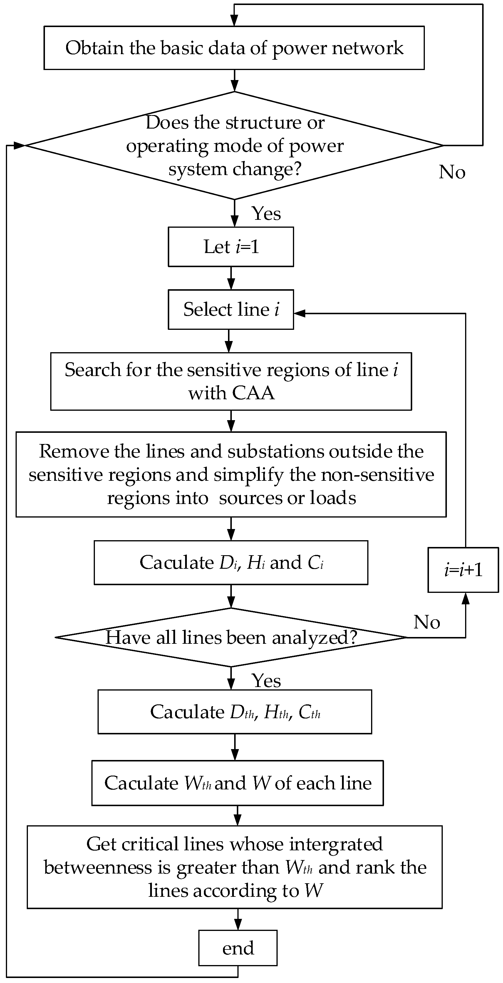
Figure 2.
(a) Power flow of the 6-bus system in normal operation; (b) The redistribution of power flow caused by the removal of line 1–3.
Figure 2.
(a) Power flow of the 6-bus system in normal operation; (b) The redistribution of power flow caused by the removal of line 1–3.
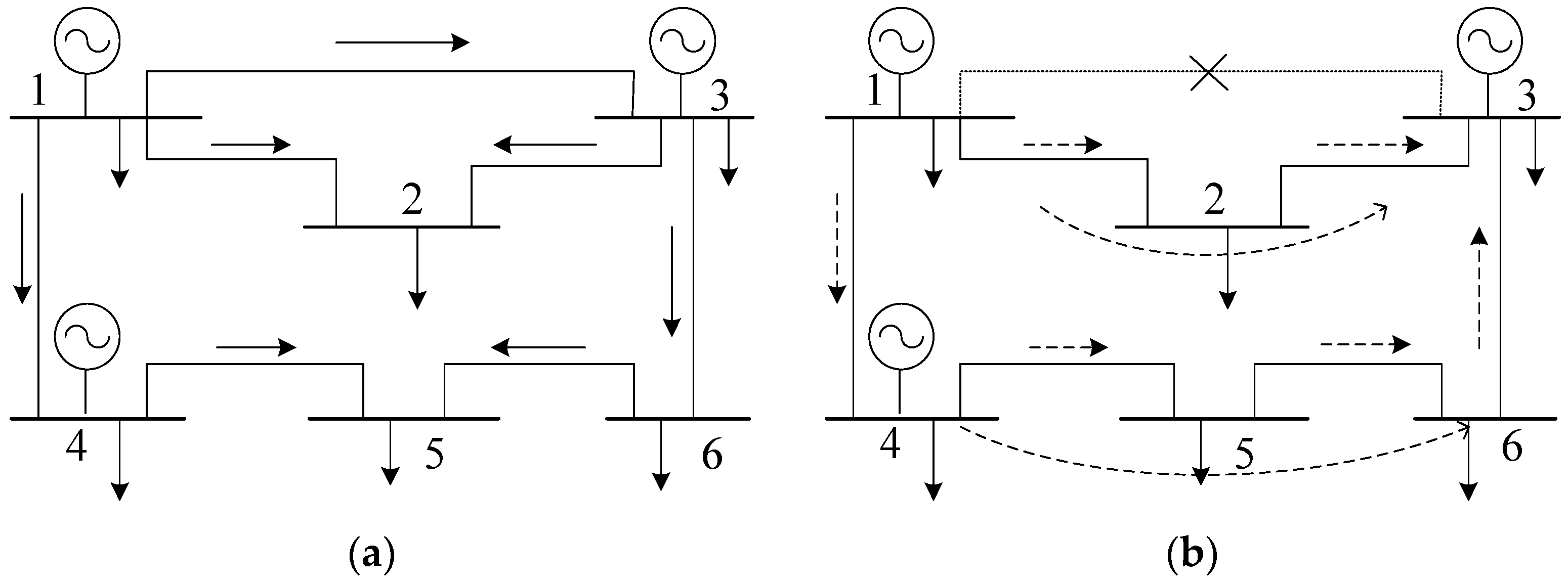
Figure 3.
The cut point in a graph.

Figure 4.
IEEE 39-bus system.
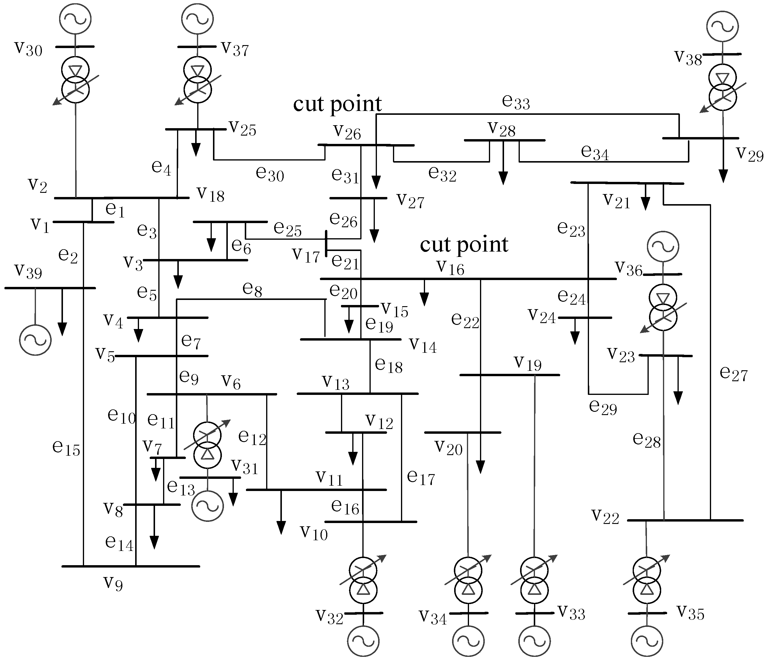
Figure 5.
Topology of sub-graph G′21.
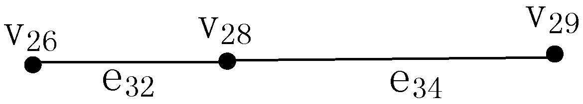
Figure 6.
(a) Increased power of transmission lines at 1.0 s when line e27 is removed at 0.5 s, De27 = 0.743978 He27 = 1 Ce27 = 0.797568 We27 = 2.541546; (b) Increased power of transmission lines at 1.0 s when line e20 is removed at 0.5 s, De20 = 0.624963 He20 = 0.38749 Ce20 = 0.930231 We20 = 1.942685; (c) Increased power of transmission lines at 1.0 s when line e29 is removed at 0.5 s, De29 = 0.052351 He29 = 0.540608 Ce29 = 0.356604 We29 = 0.949563.
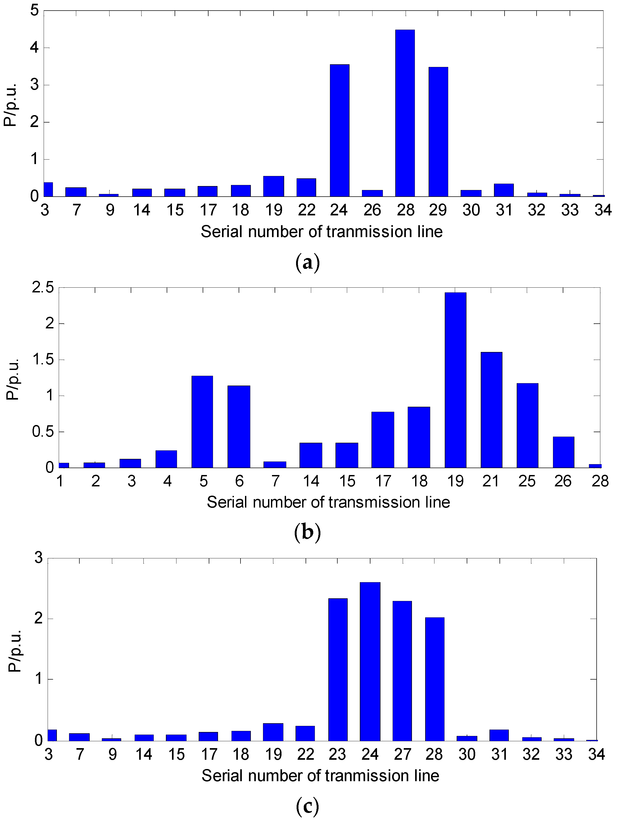
Figure 7.
(a) The number of the islands under the attacks on the first ten critical lines; (b) the total value of the loads under the attacks on the first ten critical lines; and, (c) the average probability of the incorrect tripping of remaining transmission lines under the attacks on the first ten critical lines.

Table 1.
Simulation result when line e33 is removed.
| Line | Power Change (MW) | Line | Power Change (MW) | Line | Power Change (MW) | |||
|---|---|---|---|---|---|---|---|---|
| 1 | e34 | 189.7265 | 12 | e13 | 0.584 | 23 | e2 | −0.6828 |
| 2 | e32 | 186.0633 | 13 | e10 | 0.103 | 24 | e14 | −0.6843 |
| 3 | e9 | 2.514 | 14 | e28 | 0.0099 | 25 | e6 | −0.8824 |
| 4 | e7 | 2.4037 | 15 | e29 | 0.0051 | 26 | e25 | −0.8841 |
| 5 | e26 | 2.1787 | 16 | e24 | −0.0082 | 27 | e16 | −1.2161 |
| 6 | e30 | 1.964 | 17 | e27 | −0.0305 | 28 | e12 | −1.3197 |
| 7 | e19 | 1.3781 | 18 | e23 | −0.0328 | 29 | e20 | −1.3791 |
| 8 | e18 | 1.3198 | 19 | e22 | −0.0565 | 30 | e3 | −1.4682 |
| 9 | e21 | 1.2928 | 20 | e8 | −0.0709 | 31 | e4 | −2.1515 |
| 10 | e17 | 1.2161 | 21 | e15 | −0.6759 | 32 | e31 | −2.2252 |
| 11 | e11 | 0.5896 | 22 | e1 | −0.6828 | 33 | e5 | −2.3553 |
Table 2.
Simulation result when line e20 is removed.
| Line | Power Change (MW) | Line | Power Change (MW) | Line | Power Change (MW) | |||
|---|---|---|---|---|---|---|---|---|
| 1 | e19 | 289.8958 | 12 | e31 | −63.5244 | 23 | e10 | −20.1339 |
| 2 | e21 | 288.6156 | 13 | e26 | 63.2027 | 24 | e3 | 15.7069 |
| 3 | e5 | 237.9716 | 14 | e4 | 61.5607 | 25 | e22 | 0.1593 |
| 4 | e25 | 224.116 | 15 | e9 | −48.6027 | 26 | e23 | 0.0991 |
| 5 | e6 | 222.5013 | 16 | e1 | 45.4289 | 27 | e27 | 0.0972 |
| 6 | e8 | −208.162 | 17 | e2 | 45.4289 | 28 | e28 | −0.033 |
| 7 | e18 | 81.8674 | 18 | e15 | 45.2833 | 29 | e33 | 0.0229 |
| 8 | e12 | −81.6569 | 19 | e14 | 45.1093 | 30 | e32 | −0.0216 |
| 9 | e17 | 75.1401 | 20 | e7 | −28.4259 | 31 | e34 | −0.0211 |
| 10 | e16 | −75.1401 | 21 | e11 | −25.1939 | 32 | e24 | 0.0187 |
| 11 | e30 | −63.6899 | 22 | e13 | −25.0956 | 33 | e29 | −0.0182 |
Table 3.
Calculation result of transmission lines.
| Line | Index | W | Line | Index | W | ||||||
|---|---|---|---|---|---|---|---|---|---|---|---|
| D | H | C | D | H | C | ||||||
| 1 | e27 | 0.7439 | 1 | 0.7975 | 2.5415 | 18 | e18 | 0.0749 | 0.3855 | 0.0893 | 0.5497 |
| 2 | e3 | 1 | 0.4868 | 0.8282 | 2.3150 | 19 | e17 | 0.0845 | 0.4046 | 0.0590 | 0.5482 |
| 3 | e20 | 0.6249 | 0.3874 | 0.9302 | 1.9426 | 20 | e1 | 0.0454 | 0.1499 | 0.2332 | 0.4286 |
| 4 | e31 | 0.5744 | 0.3437 | 1 | 1.9182 | 21 | e2 | 0.0454 | 0.1499 | 0.2332 | 0.4286 |
| 5 | e4 | 0.4285 | 0.3214 | 0.8308 | 1.5809 | 22 | e13 | 0.0473 | 0.2791 | 0.0370 | 0.3636 |
| 6 | e23 | 0.2676 | 0.5499 | 0.4379 | 1.2555 | 23 | e30 | 0.0042 | 0.0887 | 0.2409 | 0.3339 |
| 7 | e34 | 0.67893 | 0.3823 | 0.0890 | 1.1502 | 24 | e5 | 0.0681 | 0.1215 | 0.0919 | 0.2816 |
| 8 | e12 | 0.3574 | 0.4769 | 0.1919 | 1.0263 | 25 | e33 | 0 | 0.2001 | 0.0626 | 0.2628 |
| 9 | e21 | 0.1928 | 0.2595 | 0.5214 | 0.9738 | 26 | e7 | 0.0397 | 0.1927 | 0.0276 | 0.2601 |
| 10 | e29 | 0.0523 | 0.5406 | 0.3566 | 0.9495 | 27 | e32 | 0 | 0.1421 | 0.0322 | 0.1743 |
| 11 | e11 | 0.1849 | 0.6203 | 0.0867 | 0.8919 | 28 | e6 | 0.0517 | 0.0467 | 0.0556 | 0.1541 |
| 12 | e16 | 0.1981 | 0.4950 | 0.1285 | 0.8218 | 29 | e24 | 0.0334 | 0.0832 | 0.0055 | 0.1222 |
| 13 | e22 | 0.1972 | 0.5363 | 0.0419 | 0.7755 | 30 | e28 | 0.0329 | 0.0760 | 0.0049 | 0.1139 |
| 14 | e8 | 0.1445 | 0.3247 | 0.2794 | 0.7488 | 31 | e14 | 0.0698 | 0.0247 | 0.0047 | 0.0993 |
| 15 | e9 | 0.0232 | 0.6239 | 0.0892 | 0.7364 | 32 | e15 | 0.0698 | 0.0247 | 0.0047 | 0.0993 |
| 16 | e10 | 0.0957 | 0.4873 | 0.0881 | 0.6711 | 33 | e19 | 0.0363 | 0.0231 | 0.0013 | 0.0607 |
| 17 | e25 | 0.0434 | 0.2404 | 0.3199 | 0.6038 | 34 | e26 | 0.0014 | 0.0190 | 0.0149 | 0.0354 |
Table 4.
Calculation result of transmission lines.
| Line | W | Line | W | Line | W | Line | W | Line | W |
|---|---|---|---|---|---|---|---|---|---|
| e1 | 0.2489 | e8 | 0.5680 | e15 | 0.0955 | e22 | 1.2320 | e29 | 0.6616 |
| e2 | 0.2489 | e9 | 0.6824 | e16 | 1.0743 | e23 | 0.9019 | e30 | 0.1394 |
| e3 | 1.6463 | e10 | 0.6000 | e17 | 0.5979 | e24 | 0.1177 | e31 | 1.1108 |
| e4 | 0.9140 | e11 | 0.8219 | e18 | 0.4032 | e25 | 0.3507 | e32 | 0.1483 |
| e5 | 0.2073 | e12 | 0.9458 | e19 | 0.0597 | e26 | 0.0234 | e33 | 0.2122 |
| e6 | 0.1092 | e13 | 0.3337 | e20 | 1.1916 | e27 | 1.8976 | e34 | 1.0783 |
| e7 | 0.2291 | e14 | 0.0955 | e21 | 0.5660 | e28 | 0.1099 |
Table 5.
Calculation result of transmission lines.
| Line | W | Line | W | Line | W | Line | W | Line | W |
|---|---|---|---|---|---|---|---|---|---|
| e1 | 0.4372 | e8 | 0.7937 | e15 | 0.0993 | e22 | 1.2659 | e29 | 0.9495 |
| e2 | 0.4372 | e9 | 0.7544 | e16 | 1.1781 | e23 | 1.2555 | e30 | 0.3339 |
| e3 | 2.3150 | e10 | 0.6711 | e17 | 0.6456 | e24 | 0.1222 | e31 | 1.9182 |
| e4 | 1.5848 | e11 | 0.8919 | e18 | 0.4753 | e25 | 0.6090 | e32 | 0.1743 |
| e5 | 0.2816 | e12 | 1.1008 | e19 | 0.0607 | e26 | 0.03546 | e33 | 0.2628 |
| e6 | 0.1541 | e13 | 0.3636 | e20 | 1.9426 | e27 | 2.5415 | e34 | 1.1502 |
| e7 | 0.2514 | e14 | 0.0993 | e21 | 0.9870 | e28 | 0.1139 |
Table 6.
Computation time of different test systems.
| Test System | Number of Buses | Computation Time (s) |
|---|---|---|
| IEEE39 | 39 | 0.061 |
| IEEE118 | 118 | 0.319 |
| SYN472 | 472 | 1.285 |
| SYN1062 | 1062 | 2.891 |
| SYN3000 | 3000 | 7.639 |
| SYN7680 | 7680 | 32.268 |
| SYN12000 | 12,000 | 73.512 |
© 2017 by the authors. Licensee MDPI, Basel, Switzerland. This article is an open access article distributed under the terms and conditions of the Creative Commons Attribution (CC BY) license (http://creativecommons.org/licenses/by/4.0/).
Share and Cite
MDPI and ACS Style
Wang, Z.; He, J.; Nechifor, A.; Zhang, D.; Crossley, P. Identification of Critical Transmission Lines in Complex Power Networks. Energies 2017, 10, 1294. https://doi.org/10.3390/en10091294
AMA Style
Wang Z, He J, Nechifor A, Zhang D, Crossley P. Identification of Critical Transmission Lines in Complex Power Networks. Energies. 2017; 10(9):1294. https://doi.org/10.3390/en10091294
Chicago/Turabian StyleWang, Ziqi, Jinghan He, Alexandru Nechifor, Dahai Zhang, and Peter Crossley. 2017. "Identification of Critical Transmission Lines in Complex Power Networks" Energies 10, no. 9: 1294. https://doi.org/10.3390/en10091294
Note that from the first issue of 2016, this journal uses article numbers instead of page numbers. See further details here.