Geostatistical Three-Dimensional Modeling of a Tight Gas Reservoir: A Case Study of Block S6 of the Sulige Gas Field, Ordos Basin, China

College of Resources Science and Technology, Faculty of Geographical Science, Beijing Normal University, Beijing 100875, China
*
Authors to whom correspondence should be addressed.
Energies 2017, 10(9), 1439; https://doi.org/10.3390/en10091439
Submission received: 6 August 2017
/
Revised: 14 September 2017
/
Accepted: 15 September 2017
/
Published: 18 September 2017
Abstract
:In this study, three-dimensional (3-D) geostatistical models were constructed to quantify distributions of sandstone and mudstone. We propose a new method that employs weight coefficients to balance the sandstone and mudstone data from irregular well patterns during stochastic modeling. This new method begins with classifying well groups according to well distribution patterns; areas with similar well distribution patterns are classified within the same zone. Then, the distributions of sandstone and mudstone for each zone are simulated separately using the sequential indicator simulation (SIS) method, and the relevant variogram parameters for each zone are computed. In this paper, we used block S6 of the Sulige Gas Field in Ordos Basin in China as a case study. We evaluated the quality of each set of parameters through the vacuation checking method; certain wells were removed to generate equiprobable realizations using different seed numbers. Subsequently, the variogram parameters for the entire S6 area were obtained by assigning different weight coefficients to the parameters of each zone. Finally, a quality assessment of the sandstone and mudstone models of the S6 area was conducted using the horizontal wells, which were not involved in the stochastic modeling process. The results show that these variogram parameters, which were calculated using weight coefficients, are reliable.
1. Introduction
It’s an obvious worldwide trend that unconventional hydrocarbon accumulations are gaining more and more popularity in the oil and gas industries. Unconventional energy sources such as tight gas or oil have become essential factors that affect the energy consumption of the world [1]. It’s an associative issue to quantitatively assess unconventional gas or gas systems. As Schmoker [2] pointed out, it’s a basic approach for resource-assessment based on wells and reservoir-simulation models. Therefore, it’s necessary to establish reliable geologic models for reservoir simulation. As basic types of geologic models, sandstone and mudstone models are important, and investigating sandstone distribution provides significant information for studies related to fluvial sedimentary system in terms of flow units, physical properties, and net reservoirs. Sand body connectivity directly affects well pattern design, field development schemes, and other engineering considerations. Therefore, determining the distributions of sandstone and mudstone is key for petroleum engineering. Three-dimensional (3-D) geological modeling of sandstone and mudstone plays an important role in reservoir prediction. Geologists worldwide have performed reservoir prediction research studies based on well-logging data, dynamic testing data, seismic data, and the modern sedimentary record; modeling methods have included stochastic simulation methods such as modular neural network simulation, SIS (sequential indicator simulation), multiple-point geostatistical methods, object-based facies modeling methods, and other modeling methods. Holden et al. proposed an improved object-based method for the modeling of fluvial reservoirs conditioning on volume ratios, well observations, and seismic data [3]. Lynds and Hajek proposed a process-based conceptual model for understanding and predicting the distribution and geometries of mudstone in sandy braided-river deposits that was based on modern braided rivers and ancient braided-river deposits [4]. Deustch designed a sequential indicator simulation program named BlockSIS to gain geologically and statistically homogeneous subdivisions for soft secondary data such as porosity and permeability [5]. Pyrcz et al. designed an event-based and conditioning-flexibility program, ALLUVSIM, especially for fluvial depositional settings [6]. So far, more and more stochastic modeling methods have been created, and they have been applied to many case studies [7,8,9,10,11,12]. For the Sulige gas field, the largest onshore tight gas field, numerous reservoir geological modeling studies using different methods have been published. Jia et al. established a geological model of the sandy braided-river system for an infilling zone in Sulige gas field based on the study of outcrops in the city of Datong of Shanxi Province, and reservoir heterogeneity was analyzed [13]. Chen et al. [14,15], Zhao et al. [16], and Yang et al. [17] built geological models for Sulige gas field according to analyses of electrofacies and cores; and predictions on potential areas were made, which were summarized from numerous stochastic realizations. Han et al. [18], Wu, and Fu [19] applied the multiple-point method to build geological models for the tight gas reservoir in Sulige gas field, and horizontal wells were used to check the models’ quality. Guo et al. simulated the distributions of rock facies, sedimentary microfacies, and physical properties of the braided-river system of Sulige gas field using a particular workflow based on logging data and seismic data. Sandstone distribution models were validated by vacuation method and dynamic data [20]. However, among these studies, research specifically on sandstone and mudstone distribution is rare.
As the case studies mentioned above, the well density of the studied area was not taken into account when simulating distributions of sandstone and mudstone. When SIS is used for geological unit modeling, the distances between sampling data in the major direction (generally refer to the source direction) do affect the fitting process of the experimental variogram function. Meanwhile, within a fluvial-dominated area, there may be several sub-directions due to frequent flow changes, and it’s much more reasonable to take these sub-directions into consideration during geological modeling.
In this paper, we propose a weight-based method based on the SIS method, to describe and evaluate the sandstone and mudstone distributions of block S6 of the Sulige gas field, which will take the existing information on the irregular well patterns of this field into account and integrate directional wells with horizontal wells. Although this method is not that novel in terms of algorithm, the proposed workflow is valuable for post-processing modeling parameters. This is especially true for large-sized fields that are of good structural integrity, or for areas with greater fault development, under the condition that the fault systems formed after the reservoir was shaped.
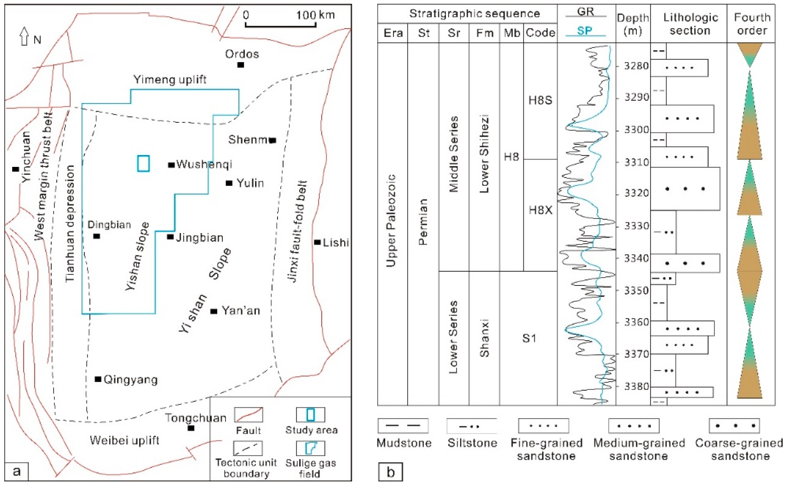
The Sulige gas field is located northwest of the Yishan Slope in Ordos Basin (Figure 1a), and its main gas-bearing formations are the Shanxi Formation and the Lower Shihezi Formation of Permian age (Figure 1b). The Sulige gas field is a tight gas field, typical to those in China, characterized by low porosity, permeability, and pressure, and high heterogeneity [1]. The study area, block S6, lies in the center of Sulige gas field, and exhibits a gentle and west-inclining monoclinal structure (Figure 1a). The target reservoirs are the Shihezi and Shanxi Formations (Figure 1b). The former is divided into two parts; the upper part includes the He1, He2, He3, and H4 members, and the lower part consists of the H5, H6, H7, and H8 members. The H8 member is subdivided into two parts: the upper member (H8S), and the lower member (H8X) (Figure 1b). The Shanxi Formation comprises the Shan1 (S1) member, and the overlying Shan2 (S2) member.
2. Materials and Method
2.1. Materials
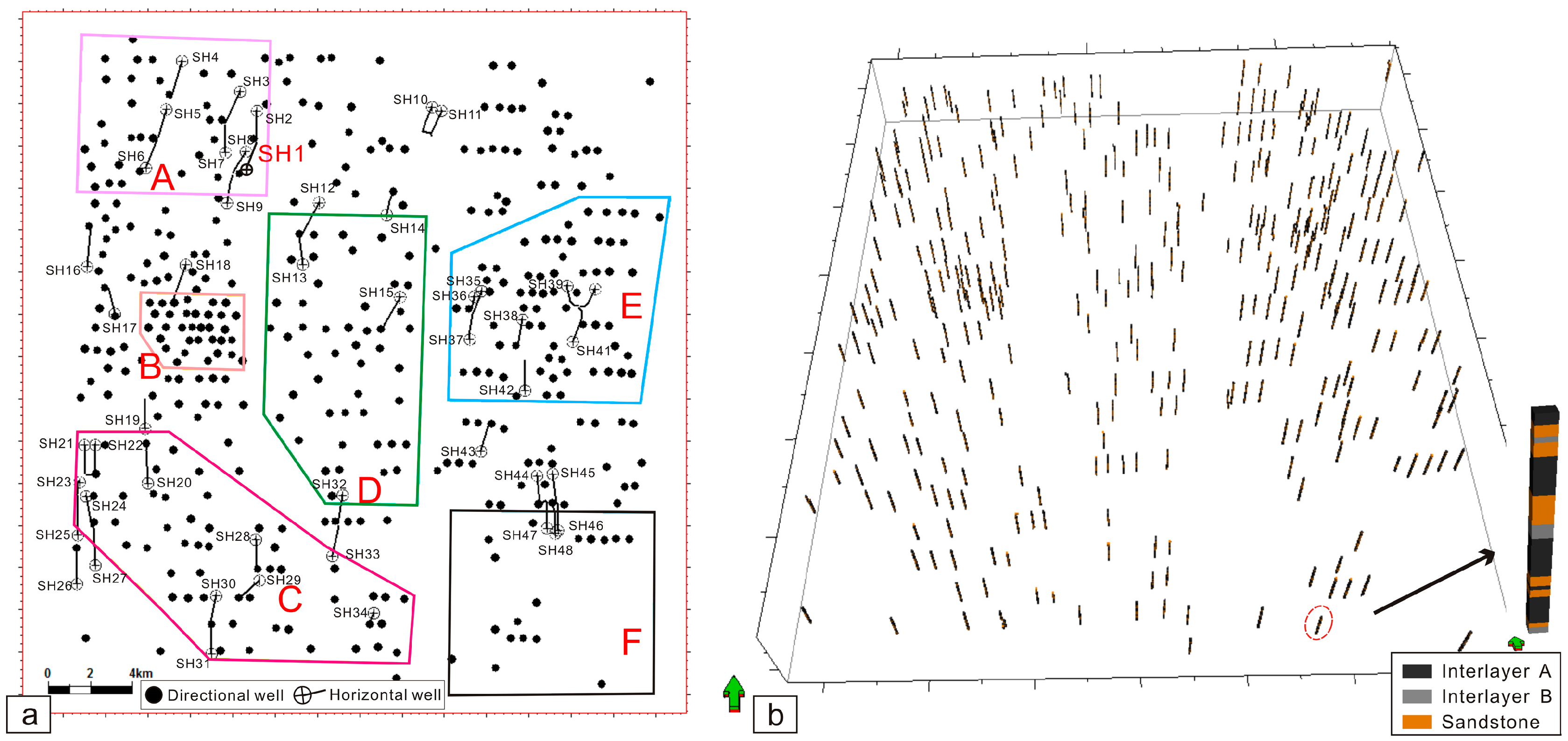
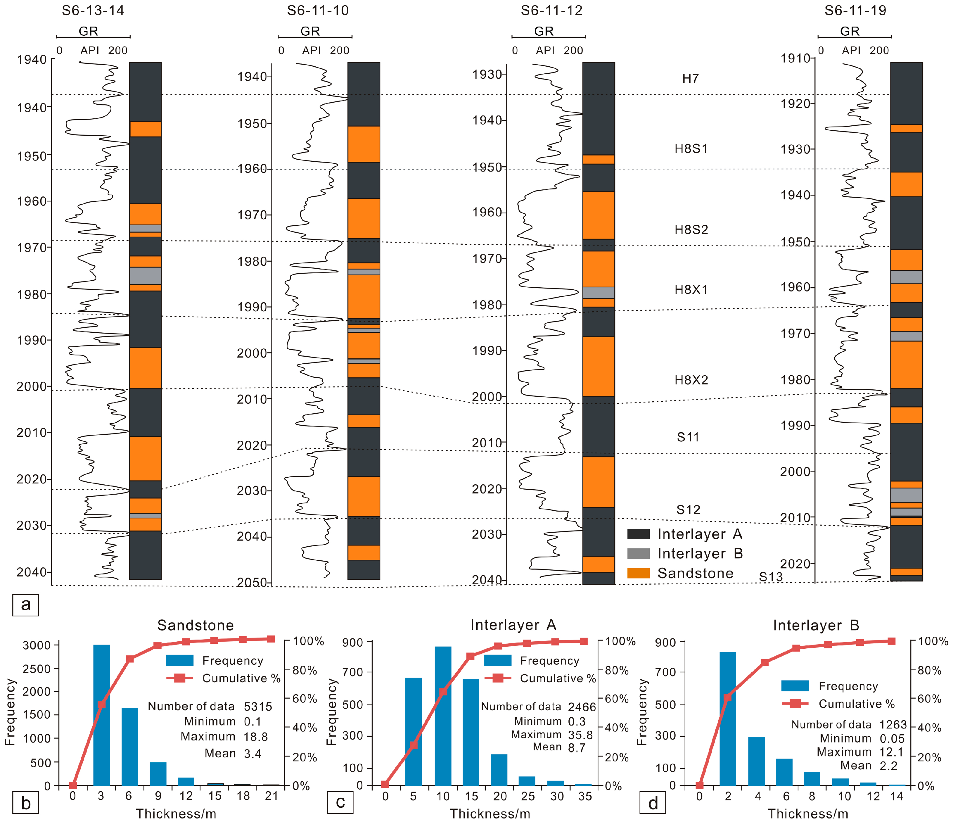
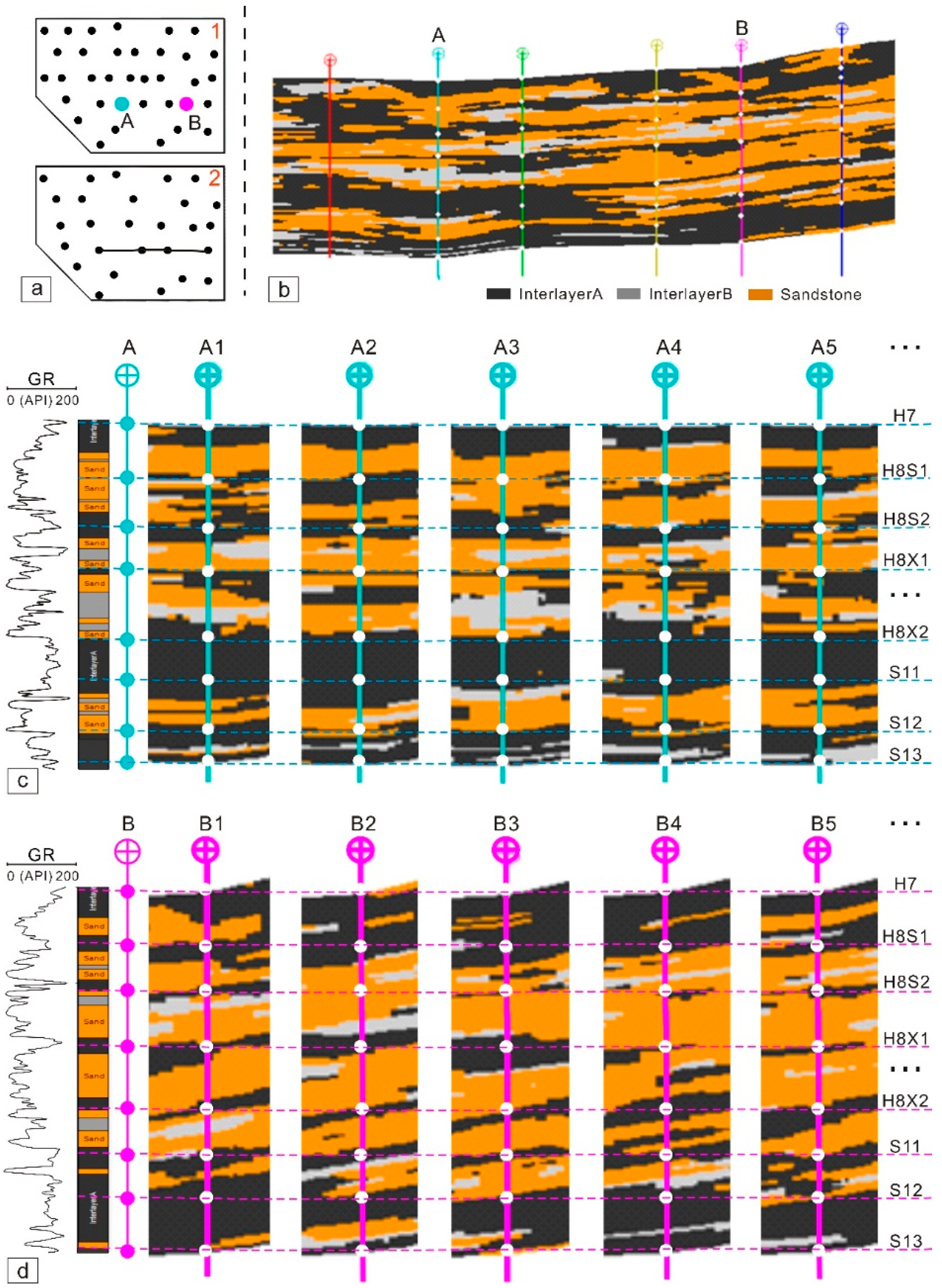
In the S6 area, a total of 390 directional wells (including the vertical wells) and 48 horizontal wells have been drilled to date (Figure 2a). All of the sandstone and mudstone interpretation data from these directional wells were used as basic data for stochastic modeling (Figure 2b). The corresponding data from the horizontal wells were not used in stochastic modeling; they were used only to verify the quality of the sandstone and mudstone model. The mudstone is subdivided into two types: interlayer A, which refers to the mudstone between two individual adjacent layers, and interlayer B, which refers to the mudstone within an individual layer (Figure 3a). This classification is based primarily on the difference in thickness between these two types of mudstone layers (Figure 3c,d). Within the study area, a total of six zones were subdivided, and their boundaries roughly determined (Figure 2a). The statistical information of these zones is shown in Table 1. According to the well density and weight coefficient data, these zones reflect the considerable heterogeneity of well distribution in the study area.
2.2. Method
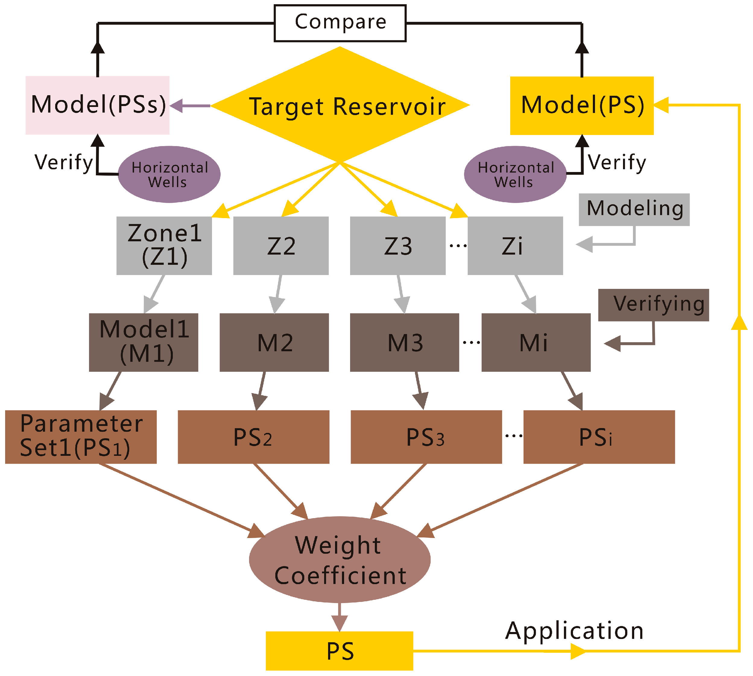
A new method based on SIS has been developed to quantitatively process the variogram parameters (major range and minor range) during stochastic modeling, and the horizontal wells were integrated to evaluate the quality of the sandstone and mudstone model (Figure 4). The SIS method was elaborately chosen for the simulation of sandstone and mudstone. The distribution or boundary of sandstone or mudstone is not simply equal to the distribution or boundary of sandy or muddy depositional elements, respectively. Moreover, the sandy depositional elements in the study area are multiple, and the boundaries between them are hard to recognize. Therefore, it’s reasonable to select SIS when there are no clear genetic shapes that could be put into object-based modeling, and the SIS models are reasonable in settings where there are no large-scale curvilinear features [5]. To implement this new approach, the target reservoir was first subdivided into several zones according to the well patterns, where areas with different well densities were classified as different zones (Figure 2a; Table 1). Then, all lithofacies (sandstone and mudstone) interpretation data from the directional wells were used to stochastically predict the sandstone and mudstone distribution for each zone to acquire the corresponding variogram parameter set. Subsequently, based on well density, each variogram parameter set was assigned different weight coefficients to obtain a variogram parameter set for the target area. The weight coefficient is defined as follows:
and the well density is calculated as follows:
- Wi—Weight coefficient of each subdivided zone;
- D—Mean well density of the target area, wells/km2;
- Di—Mean well density of the subdivided zone, wells/km2;
- N—Number of wells;
- S—Area, km2.
The final variogram parameter set (PS) for the target area was obtained via the following equation:
Thus, the variogram parameter set for the entire study area was computed directly rather than via fitting with a spherical, Gaussian, or exponential variogram model. Finally, to evaluate the quality of the sandstone and mudstone distribution models, named “model (PS)”, numerous vertical profiles of the predicted sandstone and mudstone models through the horizontal sections were made to compare with the 1-D interpretation models of horizontal sections. Meanwhile, models of sandstone and mudstone of the whole area simulated directly from the SIS method were also conducted, following the same modeling workflow of each subdomain. These kinds of models, named “model (PSs)” in the workflow, underwent the same quality checking process and were compared with model (PS). The workflow of this new method is shown in Figure 4.
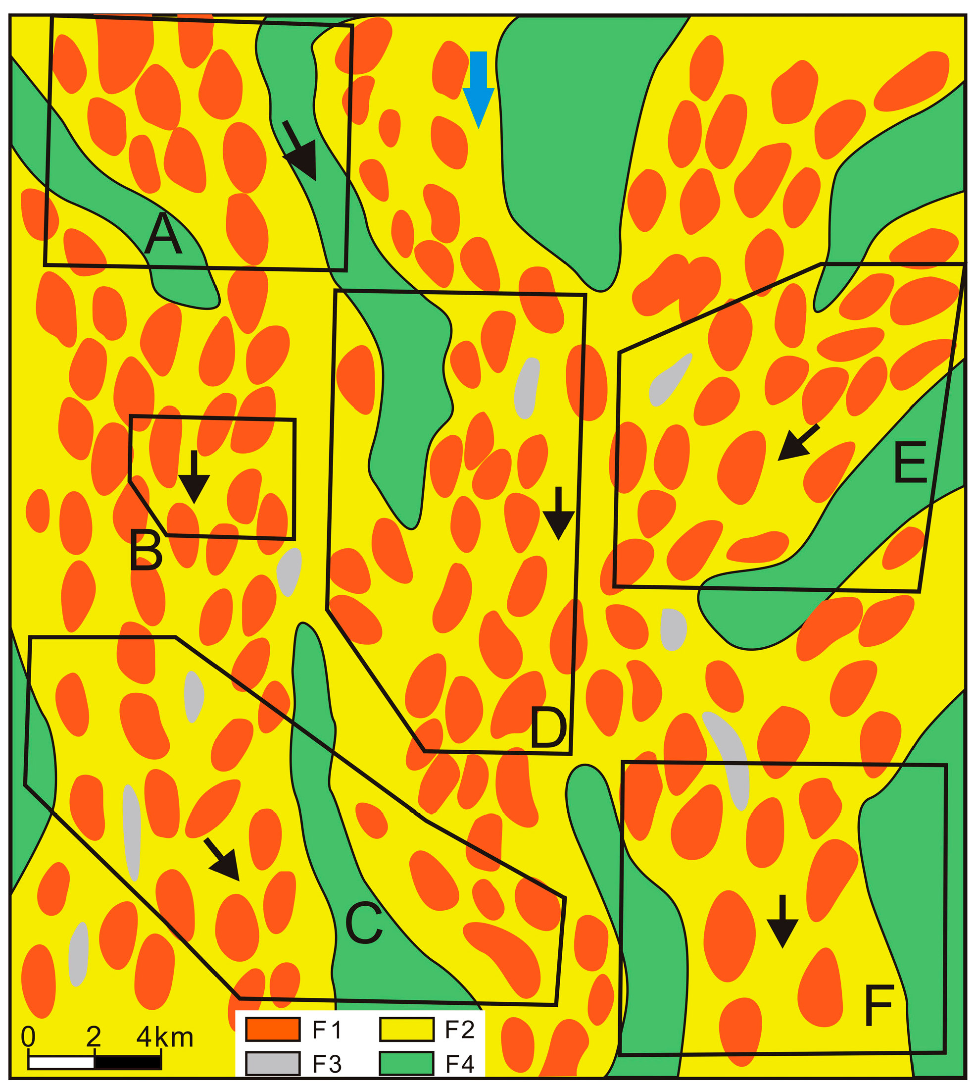
Variogram parameters are important factors when a two-point statistical simulation method is applied for geologic units modeling [5,21,22]. In fluvial reservoir modeling, distribution trends of sediments are significantly affected by the flow direction. When predicting sandstone or mudstone dimensions, it’s important and necessary to take the flow direction or source direction into account, as it has important influences on the variogram fitting, such as variogram azimuth and ranges [4,20]. As shown in Figure 5, the sandstone distributions of the five subdivided zones are characterized by different trends, which are indicated by six black arrows. If the whole area is not subdivided and the standard method is used, the variogram fitting will be affected by a united north-south tendency that is not consistent with the geological knowledge (Figure 5). However, in a geologic sense, it is more reasonable to respectively capture the ranges of variables with different directions. Therefore the proposed weight coefficient-based method subtly solves the “direction problem”.
3. Results
3.1. Sandstone and Mudstone Modeling for Subdivided Zones
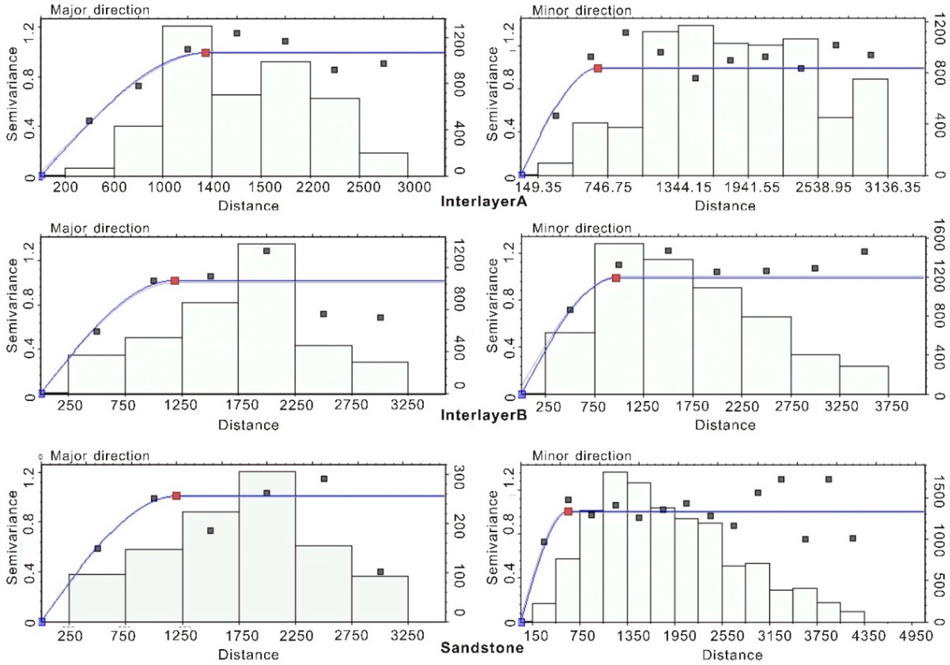
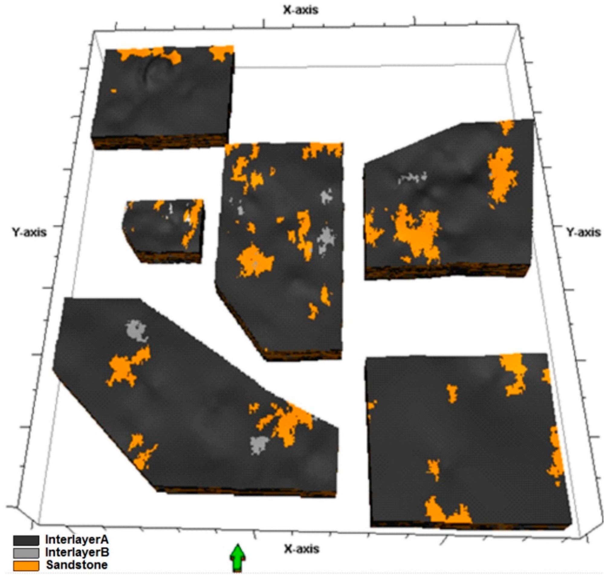
The overall structural model was upscaled into six smaller models for the subdivided zones, and subsequently, 1-D sandstone and mudstone data were discretized into each stratigraphic framework for data analysis. The SIS method was applied to sandstone and mudstone modeling based on variograms generated from lithofacies curves that represent both the horizontal and vertical distributions of proportions for each layer [11,16]. The spherical variogram model was chosen to simulate the range and 3-D spatial frequency of the sandstone and mudstone. The experimental variogram computation was completed based mainly on the average well spacing, and the spherical variogram model was then fitted to determine the major and minor ranges of sandstone and mudstone (Figure 6; Table 2). No other geological data, aside from the vertical sandstone and mudstone proportion curves, were used as constraints to make the simulated results reflect the original distribution patterns of sandstone and mudstone. Taking layer H8S1 in zone B as an example, Table 3 shows the variogram ranges of different directions that result from the variogram model fitting process (Figure 6). Ranges of sandstone and mudstone for layers in other zones were captured the same way. In this step, stochastic sandstone and mudstone distribution models for the six subdivided zones were established (Figure 7).
It is essential to verify the quality of static reservoir models to ensure that each set of variogram parameters is reliable [23,24]. The vacuation checking method [25,26], in which the data of certain wells are removed during the stochastic modeling process, was applied to evaluate the quality of the sandstone and mudstone distribution models. Only the seed number was repeatedly defined to generate equiprobable realizations to compare with the 1-D interpreted models for statistical analysis. In this paper, the quality checking results for zone B are presented. The sandstone and mudstone data of the wells shown in Figure 8(a2) were used to generate prediction models (A1, A2, …, A5 and B1, B2, …, B5), which were then used for comparison with the 1-D interpreted models, shown in the leftmost panels of Figure 8c,d. All of the prediction models are the results of using same variogram parameter sets, which are based on the original well pattern shown in Figure 8(a1). According to this comparison, the prediction distributions of interlayer A show more favorable results than those of interlayer B, which show poor connectivity between wells. The modeled distributions of sandstone are largely in accordance with the 1-D interpreted model, whereas predictions of the thin sets of sandstone are not well matched (Figure 8c,d).
In general, realizations from vacuated well data largely coincide with the 1-D interpreted data, which implies that the variogram parameter sets are reliable. The variogram parameter sets of other zones were analyzed in the same way. In this step, reasonable variogram parameter sets for each zone were obtained (Table 3). As shown in the Figure 9a,b, the ranges of the same layers of different subzones vary greatly. The variation trend represented by the dotted arrow indicates that the spatial correlation of sand bodies developed in a sandy braided river system is relatively higher when compared with other meandering intervals (H8S1, H8S2, S1-1, S1-2, and S1-3); however, their geological properties are not discussed in this paper. More details about their depositional system could refer to Zhao et al. [16] and Wang et al. [27]. This kind of correlation is consistent with the high sandstone: mudstone ratio expressed by the proposed geologic model. Figure 9c directly shows the strong heterogeneity of well numbers and well densities in six subzones. The subzone B has the highest well density among all of the subzones (Figure 9c), and both the major-direction ranges of sandstone and interlayer A are smaller than those of other subzones. Therefore, it could be inferred that variogram ranges are affected by the well patterns, and the proposed geostatistical method is meaningful.
3.2. Variogram Parameter Computations and Applications
The variogram ranges (major direction, minor direction, and vertical direction) for the entire S6 area were computed using Equation (3), and the results are shown in Table 4. All of the parameters were directly applied to generate the sandstone and mudstone distribution models for the entire S6 area (Figure 10). In this step, the spherical variogram model is used, and the seed numbers are stochastic.
3.3. Model Evaluation
The quality of models (PS) was evaluated with the assistance of horizontal wells, for which the 1-D sandstone and mudstone data were not upscaled during the stochastic modeling process. Horizontal wells in the S6 area are mainly designed to produce gas from the H8X member, and the production data show that all of these horizontal wells are capable of producing industrial gas flow. The 1-D sandstone and mudstone models of these horizontal wells were interpreted using the only available electrical logging curve, gamma ray (GR), which was captured by the logging while drilling technology. A total of 50 cross-sections of predicted sandstone and mudstone models for each horizontal well were made to compare with the corresponding 1-D interpreted sandstone and mudstone models, and three classes (I, II and III) of the comparison results were defined to evaluate the prediction models (Table 5; Figure 11). For ease of analysis, if a horizontal interval is dominated by sandstone (mudstone), the mudstone (sandstone) part is ignored when it comes to the evaluation of class II.
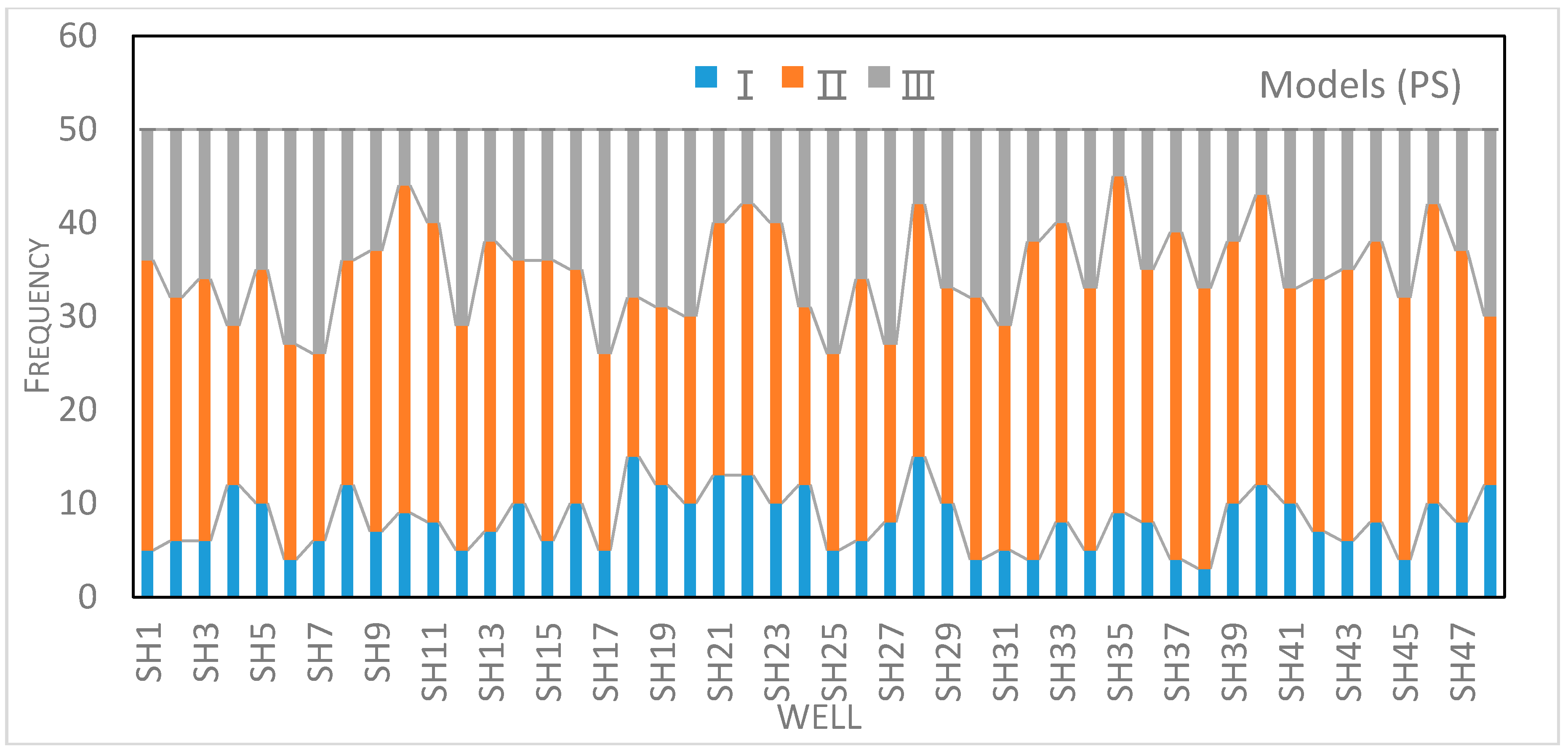
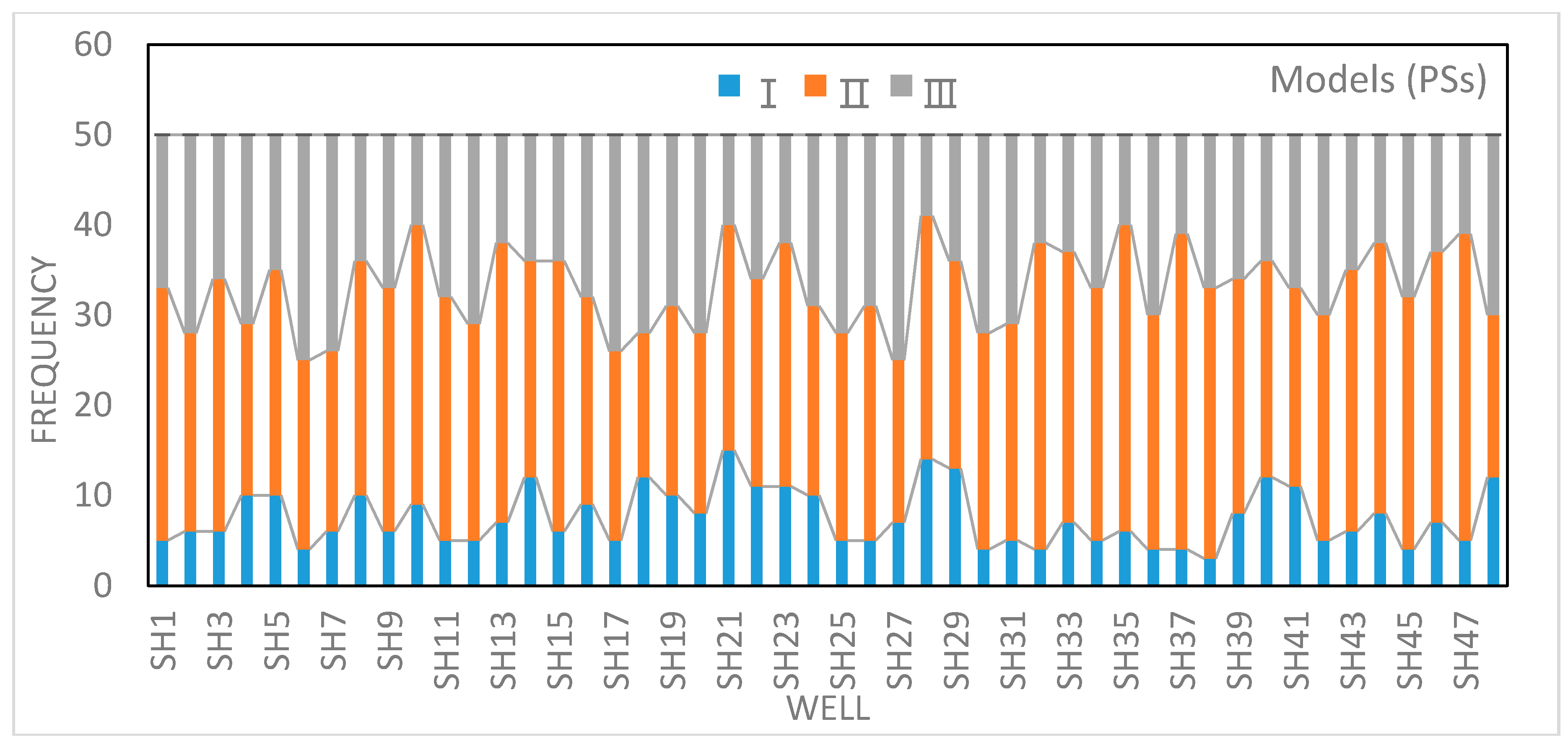
Finally, the numbers of each class of each well were collected to analyze model quality (Figure 12). Comparison between the 1-D interpreted model and models (PS) of well SH1 show that the models of type I and II account for a dominant proportion of the prediction models (Figure 12), which reflect the relatively high reliability of the variogram parameters obtained from this proposed method. Meanwhile, the same comparison for models (PSs) of well SH1 was conducted (Figure 13). As a result, types I and II are also dominant. However, the average frequencies of type I, II, and III for models (PS) and models (PSs) are different. As shown in Table 6, the average frequencies of type I and II of models (Ps) are higher than those of models (PSs), while the average frequency of type III of models (Ps) are lower than that of models (PSs). To some extent, the variogram parameters obtained from the proposed method are proved to be more reliable than the standard method.
4. Discussion
Weight coefficient-based methods of stochastic modeling for reservoirs have rarely been reported. The gentle regional structural characteristics, the sandy braided river depositional system, and the strong heterogeneity of the well distribution are all important factors that make this method feasible for this study. In terms of local tectonics, the undeveloped fault system in this region results in good structural integrity, which greatly reduces the structural uncertainty among the wells. The sandy depositional sedimentary system with a stable provenance direction is also favorable for the indicator simulation method of lithofacies. The strong heterogeneity of well distribution greatly affects the variogram model-fitting process, and to some extent, applying weight coefficients can weaken or counterbalance the influence of this type of heterogeneity on predictions. The randomly drilled horizontal wells act as an opportune evaluation tool to enable the quantitative judgment of variogram parameters. For further development in the immense Sulige gas field, this novel method can provide meaningful guidance for reservoir prediction based on 3-D geological modeling technology. Moreover, this new method is also suitable for lithofacies modeling in areas with greater fault development, under the condition that the fault systems formed after the reservoir was shaped.
However, this method still has several disadvantages. (1) Workloads are multiplied. Modeling for the same layers but for multiple zones makes the simulation procedure considerably more time-consuming. (2) Quality checking of sandstone and mudstone models for the subdivisions of zones is strictly qualitative, and the results therefore lack scientific rigor. Furthermore, the vacuation checking method only allows a small number of wells to be removed, to keep the generated models meaningful, which results in limited 1-D interpreted data available for comparison with the model predictions. Especially for zones like zone F, few wells are present, and therefore such quality checking methods are not ideal for this zone.
Because of the low porosity and permeability, and strong heterogeneity in the study area, several challenges remain for predicting sandstone and mudstone distributions in the S6 area. (1) The 3-D seismic data of the S6 area have limited coverage and, and because of the low quality of the data, they cannot be used to recognize lithofacies and distributions. (2) The quality of the static sandstone and mudstone models could hardly be effectively evaluated with the regular dynamic analysis because of the tightness of the reservoir. For example, in terms of reservoir connectivity, the effective discharge area of each well could be quantitatively evaluated using the numerical simulation method; however, the simulated results are based on the practical production data, which are controlled by the limitations of existing fracturing technology [28]. Therefore, the effective discharge area calculated with the numerical simulation does not in fact represent the inherent reservoir connectivity. In other words, the effective discharge area of a well may become larger if the fracturing technology becomes more advanced. Publications on hydraulic fractures or cracks could be referred to Rabczuk and Belytschko [29], Zhuang et al. [30], Ma et al. [31], Wang et al. [32], and Nguyen et al. [33]. Other dynamic analysis methods, such as interference tests implemented in the infill well area, face similar challenges. (3) Comparison between prediction models and 1-D interpreted models is conducted manually and semi-quantitative; the development of automatic and quantitative approaches should be prioritized in the future.
5. Conclusions
The 3-D distribution of sandstone and mudstone was modeled using the proposed weight coefficient method based on the SIS method. This new method is specifically proposed for the S6 area, where there are no faults and where wells are irregularly distributed, to balance the heterogeneity of well density for more reasonable variogram parameters. The primary variogram parameters of the six subdivided zones were determined based on the variogram model fitting, and quality controlled using the vacuation checking method. Then, 1-D interpreted sandstone and mudstone models of horizontal wells were used as standards for comparison between these models and the equiprobable realizations generated from the weight coefficient variogram parameters. The results show that types I and II are predominant among the prediction models, which indicates that the variogram parameters computed using the weight coefficient method are reliable.
Acknowledgments
This paper is supported by the Fundamental Research Funds for the Central Universities (No. 2015KJJCB11). We are grateful to Sulige Gas Field Research Center for supplying research data and offering convenience for observing cores.
Author Contributions
Jinliang Zhang gave constructive advices for the entire paper and was in decision to publish the results; Longlong Liu proposed the method and wrote the manuscript; Ruoshan Wang did some work of the interpretation of data.
Conflicts of Interest
We declare that there are no conflict of interest.
References
- Zou, C.N.; Zhai, G.M.; Zhang, G.Y.; Wang, H.J.; Zhang, G.S.; Li, J.Z.; Wang, Z.M.; Wen, Z.X.; Ma, F.; Liang, Y.B.; et al. Formation, distribution, potential and prediction of global conventional and unconventional hydrocarbon resources. Pet. Explor. Dev. 2015, 42, 13–25. [Google Scholar] [CrossRef]
- Schmoker, J.W. Resource-assessment perspectives for unconventional gas systems. AAPG Bull. 2002, 86, 1993–1999. [Google Scholar]
- Holden, L.; Hauge, R.; Skare, Ø.; Skorstad, A. Modeling of fluvial reservoirs with object models. Math. Geosci. 1998, 30, 473–496. [Google Scholar]
- Lynds, R.; Hajek, E. Conceptual model for predicting mudstone dimensions in sandy braided-river reservoirs. AAPG Bull. 2006, 90, 1273–1288. [Google Scholar] [CrossRef]
- Deutsch, C.V. A sequential indicator simulation program for categorical variables with point and block data: BlockSIS. Math. Geosci. 2006, 32, 1669–1681. [Google Scholar] [CrossRef]
- Pyrcz, M.J.; Boisvert, J.B.; Deutsch, C.V. ALLUVSIM, A program for event-based stochastic modeling of fluvial depositional systems. Math. Geosci. 2009, 35, 1671–1685. [Google Scholar] [CrossRef]
- Zheng, R.C.; Zhou, Q.; Wang, H.; Li, F.J. The sequence architecture and sandbody prediction of the second member of Shanxi formation in Changbei Gas Field, Ordos Basin. Geol. J. China Univ. 2009, 15, 69–79. [Google Scholar] [CrossRef]
- Zhang, S.; Zhu, Y.H.; Liu, H.; Wang, P.K.; Pang, S.J.; Zhao, C.C. The application of seismic waveform classification technique for sandstone prediction in shallow-water basin. Prog. Geophys. 2013, 28, 2618–2625. [Google Scholar]
- Chaki, S.; Verma, A.K.; Routray, A.; Mohanty, W.K. Well tops guided prediction of reservoir properties using modular neural network concept, a case study from western onshore, India. J. Pet. Sci. Eng. 2014, 123, 155–163. [Google Scholar] [CrossRef]
- Dong, G.Y.; He, Y.B.; Leng, C.P.; Gao, L.F. Mechanism of sand body prediction in a continental rift basin by coupling paleogeomorphic elements under the control of base level. Pet. Explor. Dev. 2016, 43, 579–590. [Google Scholar] [CrossRef]
- Liu, L.L.; Zhang, J.L.; Wang, R.S.; Wang, J.K.; Yu, J.T.; Sun, Z.Q.; Wang, G.Q.; Guo, J.Q.; Liu, S.S.; Zhang, P.H. Facies architectural analysis and three-dimensional modeling of Wen79 fault block, Wenliu oilfield, Dongpu depression, China. Arab. J. Geosci. 2016, 9, 714. [Google Scholar] [CrossRef]
- Yin, X.D.; Lu, S.F.; Wang, P.F.; Wang, Q.M.; Wang, W.; Yao, T.Y. A three-dimensional high-resolution reservoir model of the Eocene Shahejie formation in Bohai Bay Basin, integrating stratigraphic forward modeling and geostatistics. Mar. Pet. Geol. 2017, 82, 362–370. [Google Scholar] [CrossRef]
- Jia, A.L.; Tang, J.W.; He, D.B.; Ji, Y.K.; Cheng, L.H. Geological modeling for sandstone reservoirs with low permeability and strong heterogeneity in sulige gas field. China Pet. Explor. 2007, 1, 12–16. [Google Scholar]
- Chen, F.X.; Lu, T.; Da, S.P.; Xu, X.R.; Tang, L.P. Study on sedimentary facies of braided stream and its application in geological modeling in sulige gas field. Pet. Geol. Eng. 2008, 22, 21–24. [Google Scholar]
- Chen, F.X.; Wang, Y.; Zhang, J.; Yang, Y. He8 reservoir’s favorable development blocks in Sulige gas field, Ordos Basin. Nat. Gas Geosci. 2009, 20, 95–99. [Google Scholar]
- Zhao, Y.; Li, J.B.; Zhang, J.; Zhang, Q. Methodology for geologic modeling of low-permeability fluvial sandstone reservoirs and its application: A case study of the Su-6 infilling drilling pilot in the Sulige gas field. Nat. Gas Ind. 2010, 30, 32–35. [Google Scholar]
- Yang, R.C.; Wang, Y.L.; Fan, A.P.; Han, Z.Z.; Ma, D.X.; Wang, X.P.; Gao, F.L. Reservoir geological modeling of Z30 block in Sulige gas field, Ordos Basin. Nat. Gas Ind. 2012, 23, 1148–1154. [Google Scholar]
- Han, J.C.; Wang, X.B.; Sun, Z.X.; Li, Z.Y. Simulation of fluvial sedimentary microfacies using multiple-point geostatistics. Spec. Oil Gas Reserv. 2011, 18, 48–51. [Google Scholar]
- Wu, T.; Fu, B. Application of the multiple-point method to geological modeling in the Sulige gas field. Geol. Explor. 2016, 52, 0985–0991. [Google Scholar]
- Guo, Z.; Sun, L.D.; Jia, A.L.; Lu, T. 3-D geological modeling for tight sand gas reservoir of braided river facies. Pet. Explor. Dev. 2015, 42, 83–91. [Google Scholar] [CrossRef]
- Journel, A.G.; Isaaks, E.H. Conditional indicator simulation: Application to a Saskatchewan uranium deposit. Math. Geosci. 1984, 16, 685–718. [Google Scholar] [CrossRef]
- Goovaerts, P. Comparative performance of indicator algorithms for modeling conditional probability distribution functions. Math. Geosci. 1994, 26, 385–410. [Google Scholar] [CrossRef]
- Zhang, J.L.; Dong, Z.R.; Li, D.Y. A Reservoir Assessment of the Qingshankou Sandstones (The Upper Cretaceous), Daqingzijing Field, South Songliao Basin, Northeastern China. Pet. Sci. Technol. 2014, 32, 274–280. [Google Scholar] [CrossRef]
- Liu, L.L.; Zhang, J.L.; Wang, J.K.; Li, C.L.; Yu, J.T.; Zhang, G.X.; Fan, Z.L.; Wei, G.Q.; Sun, Z.Q.; Xue, H.H.; et al. Geostatistical modeling for fine reservoir description of Wei2 block of Weicheng oilfield, Dongpu depression, China. Arab. J. Geosci. 2015, 8, 9101–9115. [Google Scholar] [CrossRef]
- Hou, J.G.; Xu, S.Y. Stochastic simulation methods analysis of channel sandstone reservoir. Pet. Explor. Dev. 1998, 25, 62–64. [Google Scholar]
- Yin, Y.S.; Wu, S.H.; Zhang, C.M.; Li, S.H.; Zhang, S.F. Integrative prediction of microfacies with multiple stochastic modeling methods. Acta Pet. Sin. 2006, 27, 68–71. [Google Scholar]
- Wang, J.P.; Ren, Z.L.; Shan, J.F.; Zhu, Y.J. He8 and Shan1 members’ depositional system research. Geol. Sci. Technol. Inf. 2011, 30, 41–48. [Google Scholar]
- Tang, M.M.; Zhang, J.L. Fracture Modeling and Application Based on fracture Mechanics; Martinus Nijhoff Publishers: Leydent, The Netherlands, 2010. [Google Scholar]
- Rabczuk, T.; Belytschko, T. A three-dimensional large deformation meshfree method for arbitrary evolving cracks. Comput. Methods Appl. Mech. Eng. 2007, 196, 2777–2799. [Google Scholar] [CrossRef]
- Zhuang, X.; Huang, R.; Rabczuk, T.; Liang, C. A coupled thermo-hydro-mechanical model of jointed hard rock for compressed air energy storage. Math. Probl. Eng. 2014, 2014, 179169. [Google Scholar] [CrossRef]
- Ma, X.; Hao, R.F.; Lai, X.A.; Zhang, Y.M.; Ma, Z.G.; He, M.F.; Xiao, Y.X.; Bi, M.; Ma, X.X. Field test of volume fracturing for horizontal wells in Sulige tight sandstone gas reservoirs, NW China. Pet. Explor. Dev. 2014, 41, 810–816. [Google Scholar] [CrossRef]
- Wang, J.K.; Zhang, J.L.; Xie, J.; Ding, F. Initial gas full-component simulation experiment of Ban-876 underground gas storage. J. Nat. Gas Sci. Eng. 2014, 18, 131–136. [Google Scholar] [CrossRef]
- Nguyen, V.P.; Lian, H.; Rabczuk, T.; Bordas, S. Modelling hydraulic fractures in porous media using flow cohesive interface elements. Eng. Geol. 2017, 225, 68–82. [Google Scholar] [CrossRef]
Figure 1.
(a) Location map of S6 area in Sulige gas field; (b) Stratigraphy of upper Paleozoic; only the H8 and S1 layers are shown.
Figure 1.
(a) Location map of S6 area in Sulige gas field; (b) Stratigraphy of upper Paleozoic; only the H8 and S1 layers are shown.

Figure 2.
(a) Classification of the subdivided zones, showing the locations of directional wells and horizontal wells. While subdividing, the boundaries of the six zones are roughly drawn; (b) Discretized sandstone/mudstone data used as input data for stochastic modeling.
Figure 2.
(a) Classification of the subdivided zones, showing the locations of directional wells and horizontal wells. While subdividing, the boundaries of the six zones are roughly drawn; (b) Discretized sandstone/mudstone data used as input data for stochastic modeling.

Figure 3.
(a) 1-D interpreted sandstone and mudstone data of four directional wells; (b–d) Statistical histograms of sandstone, interlayer A, and interlayer B, respectively. Note that the mean thicknesses of interlayer A and interlayer B are quite different.
Figure 3.
(a) 1-D interpreted sandstone and mudstone data of four directional wells; (b–d) Statistical histograms of sandstone, interlayer A, and interlayer B, respectively. Note that the mean thicknesses of interlayer A and interlayer B are quite different.

Figure 4.
Workflow of the weight coefficient method of modeling sandstone and mudstone distribution.
Figure 4.
Workflow of the weight coefficient method of modeling sandstone and mudstone distribution.

Figure 5.
Different types of sand bodies and mudstone distribution trends of the subdivided zones. The different trends are indicated by six black arrows and the blue arrow refers to the general source direction of the study area. F1 and F2 refer to the sandy facies, F3 and F4 refer to the muddy facies.

Figure 6.
Variogram model fitting of sandstone and mudstone for layer H8S1 in zone B.

Figure 7.
3-D sandstone and mudstone distribution models for the six subdivided zones. It’s noted that each distribution model is just one of the equiprobable realizations.
Figure 7.
3-D sandstone and mudstone distribution models for the six subdivided zones. It’s noted that each distribution model is just one of the equiprobable realizations.

Figure 8.
(a) The original (the upper one) and the vacuated well pattern (the lower one), showing the locations of eight removed wells; (b) Cross-section of sandstone and mudstone model, within which well A and well B did not participate in the modeling process; section location is drawn in Figure 8(a2); (c,d) Comparison between five stochastic realizations or prediction models (A1, A2, …, A5 and B1, B2, …, B5) and 1-D interpreted sandstone and mudstone model of well A and well B, respectively.

Figure 9.
Relationships between layers and major direction ranges of different subzones. As shown in the figure, both the major direction ranges of sandstone and interlayer A for the six subzones are characterized by obvious horizontal and vertical fluctuations. (a) The ranges of sandstone for the braided intervals H8X1 and H8X2 are relatively larger than those for the meandering intervals (H8S1, H8S2, S1-1, S1-2 and S1-3); (b) The ranges of interlayer A for the braided intervals are relatively smaller than those for the meandering intervals; (c) Statistics of well numbers and well densities for the six subzones.
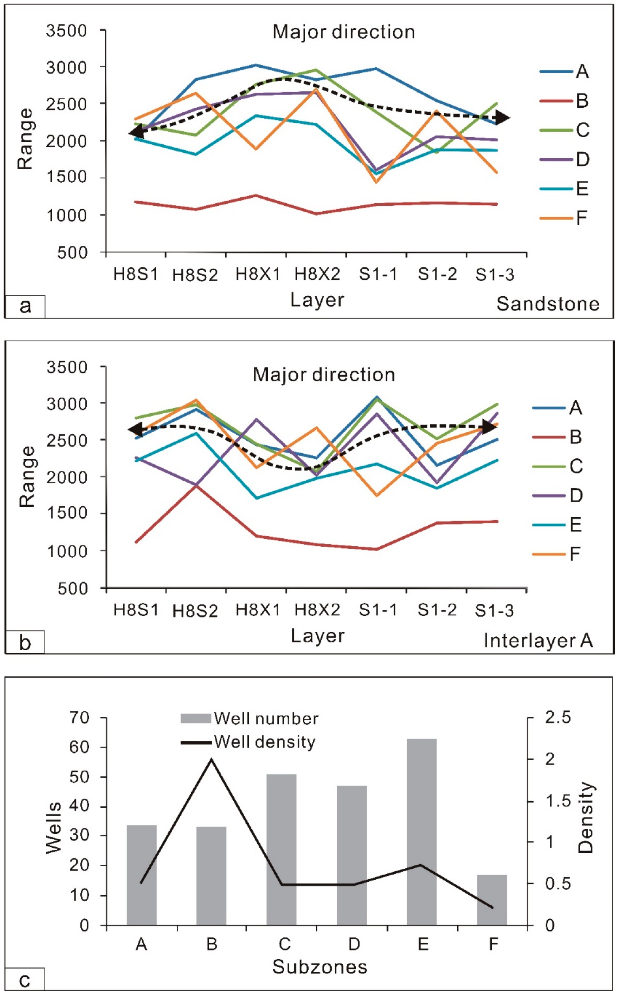
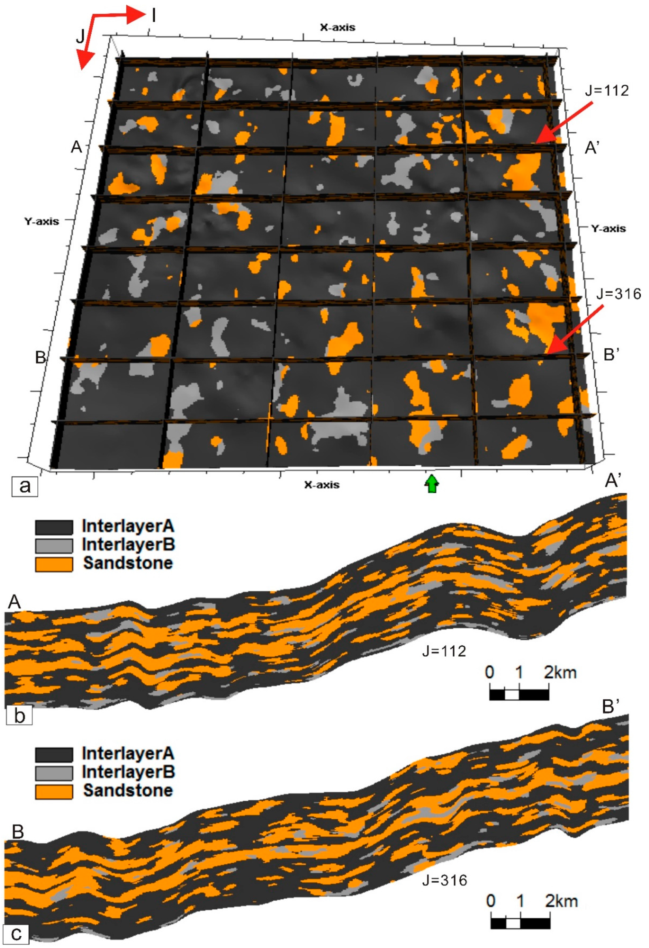
Figure 10.
(a) 3-D cut slices of the entire S6 area at I (or X-axis) direction (5, 76, 147, 218, 289, 360) and J (or Y-axis) direction (10, 61, 112, 163, 214, 265, 316, 367); (b,c) Magnified cross-section of J = 112 and J = 316, respectively.
Figure 10.
(a) 3-D cut slices of the entire S6 area at I (or X-axis) direction (5, 76, 147, 218, 289, 360) and J (or Y-axis) direction (10, 61, 112, 163, 214, 265, 316, 367); (b,c) Magnified cross-section of J = 112 and J = 316, respectively.

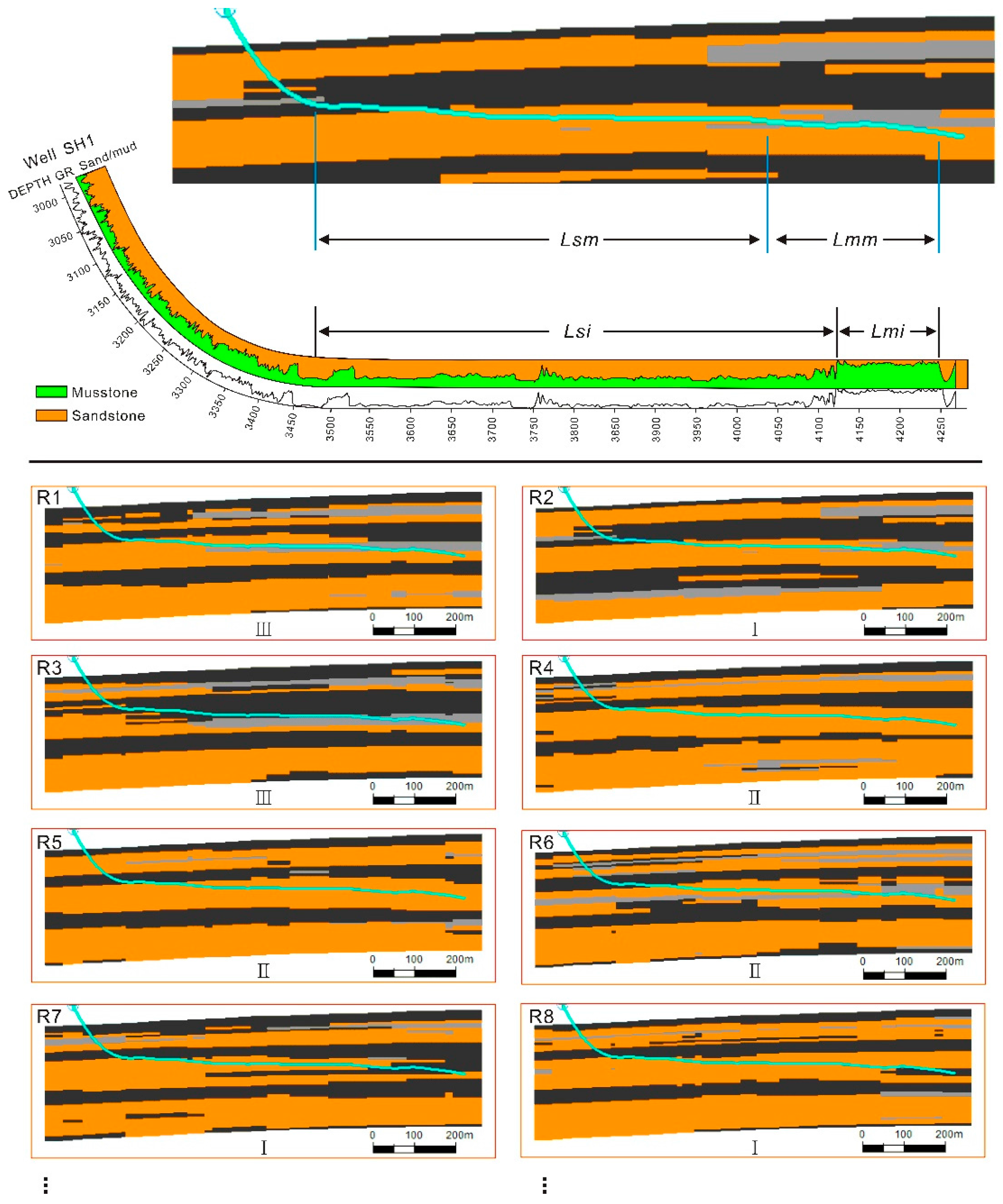
Figure 11.
Classified cross-sections of prediction models for horizontal well SH1. The uppermost figure is a cross-section of a simulated sandstone and mudstone model, and the lower figure next to it is the 1-D interpreted sandstone and mudstone model. The lowest cross-sections are eight stochastic realizations (R1, R2, ..., R8) generated via the same variogram parameters, but using different seed numbers. The location of horizontal well SH1 is shown in Figure 2a. Lsm (Lmm) refers to the length of sandstone (mudstone) obtained from stochastic modeling; Lsi (Lmi) refers to the length of sandstone (mudstone) obtained from well logging interpretation.

Figure 12.
Statistics of comparison results of 48 horizontal wells in S6 area. These comparison results are based on the proposed method. As is shown in the Figure, type I and II are dominant.
Figure 12.
Statistics of comparison results of 48 horizontal wells in S6 area. These comparison results are based on the proposed method. As is shown in the Figure, type I and II are dominant.

Figure 13.
Statistics of comparison results of 48 horizontal wells in S6 area. These comparison results are based on the standard SIS method. Frequencies of type I and II are similar to those of models (PS).
Figure 13.
Statistics of comparison results of 48 horizontal wells in S6 area. These comparison results are based on the standard SIS method. Frequencies of type I and II are similar to those of models (PS).


Table 1.
Well densities of six zones and the whole study area.
| Zones | S (km2) | N | D (wells/km2) |
|---|---|---|---|
| A | 65.70 | 34 | 0.52 |
| B | 16.50 | 33 | 2.00 |
| C | 104.70 | 51 | 0.49 |
| D | 95.10 | 47 | 0.49 |
| E | 85.80 | 63 | 0.73 |
| F | 82.90 | 17 | 0.21 |
| Six zones | 450.70 | 245 | - |
| The whole area | 956.70 | 390 | 0.41 |
Table 2.
Data used to model distribution of sandstone and mudstone for layer H8S1 in zone B.
| Lithofacies | Variogram Ranges | Variogram Type | |||
|---|---|---|---|---|---|
| Major Direction | Minor Direction | Vertical Direction | Azimuth (°) | ||
| Interlayer A | 1347.1 | 661.4 | 9.5 | 10 | Spherical model |
| Interlayer B | 1185.3 | 965.4 | 3.9 | 7 | Spherical model |
| Sandstone | 1176.7 | 782.6 | 8.5 | 9 | Spherical model |
Table 3.
Varaiogram parameters for the six subdivided zones.
| Zone | Facies | Variogram Ranges | ||||||||||||||||||||
|---|---|---|---|---|---|---|---|---|---|---|---|---|---|---|---|---|---|---|---|---|---|---|
| H8S1 | H8S2 | H8X1 | H8X2 | S1-1 | S1-2 | S1-3 | ||||||||||||||||
| Maj | Min | Ver | Major | Min | Ver | Maj | Min | Ver | Maj | Min | Ver | Maj | Min | Ver | Maj | Min | Ver | Maj | Min | Ver | ||
| A | Interlayer A | 2521.9 | 2471.1 | 8.8 | 2911.8 | 2475.2 | 7.4 | 2436 | 2049.6 | 9.2 | 2255.6 | 2064.5 | 9.1 | 3080.9 | 1629.2 | 8.8 | 2155.1 | 1791.9 | 7.5 | 2505.6 | 2096.2 | 7.9 |
| Interlayer B | 2326.5 | 2114.0 | 2.9 | 2107.1 | 1758.3 | 2.2 | 1775 | 1420.4 | 3.4 | 2176.0 | 1607.1 | 3.4 | 2399.2 | 1767.4 | 2.7 | 1742.4 | 1400.0 | 4.7 | 2327.2 | 2194.1 | 5.9 | |
| Sandstone | 2021.7 | 1911.0 | 5.4 | 2825.6 | 1842.6 | 7.0 | 3022 | 1917.4 | 6.6 | 2824.0 | 1944.8 | 7.6 | 2973.6 | 1840.7 | 7.7 | 2543.9 | 1993.1 | 5.4 | 2228.8 | 1920.1 | 7.1 | |
| B | Interlayer A | 1347.1 | 661.4 | 9.5 | 1877.6 | 998.7 | 9.3 | 1196 | 784.1 | 7.5 | 1078.3 | 860.1 | 7.6 | 1016.3 | 982.6 | 7.7 | 1373.2 | 907.3 | 9.6 | 1392.8 | 1201.9 | 5.3 |
| Interlayer B | 1185.3 | 965.4 | 3.9 | 1091.6 | 411.7 | 3.0 | 593 | 401.3 | 2.7 | 926.6 | 669.7 | 2.5 | 988.7 | 895.2 | 3.3 | 907.2 | 587.5 | 5.0 | 1191.2 | 680.9 | 4.6 | |
| Sandstone | 1176.7 | 782.6 | 8.5 | 1073.1 | 830.9 | 5.5 | 1262 | 1050.9 | 4.9 | 1017.1 | 761.0 | 6.1 | 1138.3 | 958.7 | 6.5 | 1162.2 | 829.0 | 5.7 | 1144.8 | 846.9 | 8.2 | |
| C | Interlayer A | 2795.2 | 2197.0 | 7.9 | 2978.5 | 2192.3 | 13 | 1144 | 1276.4 | 7.1 | 2072.7 | 1256.3 | 8.7 | 3046.8 | 1551.8 | 8.4 | 2513.0 | 1835.4 | 7.9 | 2984.4 | 2110.1 | 9.8 |
| Interlayer B | 2240.5 | 2453.5 | 4.5 | 2419.9 | 1703.6 | 3.3 | 2517 | 2234.7 | 3.3 | 1416.2 | 1358.2 | 3.5 | 1978.9 | 1539.6 | 3.3 | 2357.3 | 1586.3 | 4.8 | 2426.1 | 1766.4 | 3.7 | |
| Sandstone | 2227.9 | 1634.5 | 5.5 | 2076.6 | 1755.2 | 5.0 | 2760 | 2238.3 | 5.4 | 2955.5 | 2109.5 | 7.4 | 2388.9 | 2215.1 | 8.2 | 1841.6 | 1587.0 | 6.4 | 2503.1 | 1802.3 | 4.0 | |
| D | Interlayer A | 2258.2 | 1877.7 | 8.0 | 1889.8 | 1876.4 | 8.3 | 2775 | 1662.0 | 6.8 | 2019.8 | 1956.7 | 5.8 | 2852.4 | 1651.5 | 9.6 | 1920.4 | 1575.1 | 8.9 | 3060.5 | 2338.0 | 6.9 |
| Interlayer B | 1412.8 | 810.3 | 4.1 | 1749.8 | 1321.4 | 4.7 | 2641 | 999.7 | 2.7 | 1267.9 | 886.3 | 3.5 | 2526.5 | 1893.3 | 4.3 | 2200.9 | 714.4 | 4.9 | 2666.7 | 2586.9 | 4.1 | |
| Sandstone | 2127.2 | 1311.6 | 4.9 | 2427.1 | 1974.2 | 7.4 | 2628 | 2192.8 | 5.8 | 2649.9 | 2026.5 | 7.3 | 1607.4 | 706.6 | 7.4 | 2055.3 | 1855.6 | 6.1 | 2012.6 | 1042.9 | 3.4 | |
| E | Interlayer A | 2217.1 | 1338.1 | 6.9 | 2588.4 | 844.8 | 7.8 | 1708 | 1098.1 | 7.8 | 1978.7 | 1239.4 | 6.4 | 2175.0 | 1372.7 | 7.5 | 1845.2 | 1301.5 | 7.5 | 2223.2 | 1564.8 | 8.4 |
| Interlayer B | 2038.2 | 1942.1 | 3.0 | 1204.6 | 895.0 | 4.2 | 1074 | 835.0 | 2.9 | 1783.4 | 967.5 | 3.3 | 1749.1 | 1073.7 | 5.5 | 1663.8 | 881.9 | 5.7 | 2151.8 | 1050.5 | 6.4 | |
| Sandstone | 2025.2 | 1593.7 | 6.6 | 1315.3 | 1058.5 | 5.4 | 2338 | 2115.1 | 6.1 | 2219.4 | 1109.1 | 4.2 | 1556.2 | 1067.5 | 6.5 | 1880.3 | 741.9 | 5.6 | 1872.4 | 1003.0 | 2.7 | |
| F | Interlayer A | 2582.5 | 2306.9 | 5.9 | 3038.2 | 2246.6 | 6.7 | 2123 | 1945.9 | 6.7 | 2663.0 | 1701.5 | 5.5 | 1744.7 | 1483.1 | 6.1 | 2453.6 | 2414.6 | 8.4 | 2713.3 | 1951.2 | 5.2 |
| Interlayer B | 2177.9 | 1582.5 | 2.0 | 2654.2 | 1845.7 | 5.7 | 2095 | 1790.7 | 4.1 | 2190.0 | 1674.0 | 6.2 | 1610.5 | 948.3 | 6.3 | 2406.1 | 2309.1 | 3.8 | 2209.8 | 1737.8 | 1.5 | |
| Sandstone | 2292.9 | 1349.1 | 5.3 | 2642.9 | 2079.1 | 4.5 | 1889 | 1154.7 | 7.7 | 2692.8 | 1694.2 | 7.0 | 1440.7 | 998.1 | 5.5 | 2402.7 | 2154.3 | 6.3 | 1576.0 | 1229.9 | 2.3 | |
Table 4.
Computed variogram ranges for the entire zone.
| Facies | Variogram Range | |||||||||||
|---|---|---|---|---|---|---|---|---|---|---|---|---|
| H8S1 | H8S2 | H8X1 | H8X2 | |||||||||
| Maj | Min | Ver | Maj | Min | Ver | Maj | Min | Ver | Maj | Min | Ver | |
| Interlayer A | 2492.3 | 2089.6 | 7.8 | 2609.1 | 2050.7 | 9.4 | 2050.2 | 1610.9 | 7.5 | 2143.5 | 1677.0 | 7.4 |
| Interlayer B | 1979.7 | 1741.2 | 3.6 | 2077.2 | 1542.4 | 3.8 | 2213.3 | 1520.8 | 3.2 | 1644.0 | 1271.6 | 3.8 |
| Sandstone | 2132.1 | 1550.2 | 5.4 | 2333.6 | 1811.1 | 6.1 | 2622.8 | 2004.1 | 6.1 | 2725.6 | 1909.1 | 7.1 |
| S1-1 | S1-2 | S1-3 | ||||||||||
| Interlayer A | 2752.0 | 1567.9 | 8.5 | 2191.8 | 1765.3 | 8.2 | 2794.5 | 2102.0 | 7.8 | |||
| Interlayer B | 2153.6 | 1578.7 | 4.0 | 2115.0 | 1310.7 | 4.8 | 2411.9 | 2025.0 | 4.2 | |||
| Sandstone | 2095.2 | 1451.4 | 7.4 | 2111.3 | 1745.0 | 6.0 | 2127.7 | 1466.6 | 4.3 | |||
Table 5.
Evaluation criterion for prediction model.
| Classification | Evaluation Formula | Evaluation Criterion | |
|---|---|---|---|
| Sandstone | Mudstone | ||
| I | Ps = Lsm/Lsi | Pm = Lmm/Lmi | Ps ≥ 0.8 and Pm ≥ 0.8 |
| II | 0.6 ≤ Ps < 0.8 (Sandstone dominated); 0.6 ≤ Pm < 0.8 (Mudstone dominated) | ||
| III | Others | ||
Table 6.
Average frequencies of type I, II, and III for models (PS) and models (PSs).
| Average frequency | |||
|---|---|---|---|
| I | II | III | |
| Models (PS) | 8.2 | 26.6 | 15.2 |
| Models (PSs) | 7.5 | 25.6 | 16.9 |
© 2017 by the authors. Licensee MDPI, Basel, Switzerland. This article is an open access article distributed under the terms and conditions of the Creative Commons Attribution (CC BY) license (http://creativecommons.org/licenses/by/4.0/).
Share and Cite
MDPI and ACS Style
Zhang, J.; Liu, L.; Wang, R. Geostatistical Three-Dimensional Modeling of a Tight Gas Reservoir: A Case Study of Block S6 of the Sulige Gas Field, Ordos Basin, China. Energies 2017, 10, 1439. https://doi.org/10.3390/en10091439
AMA Style
Zhang J, Liu L, Wang R. Geostatistical Three-Dimensional Modeling of a Tight Gas Reservoir: A Case Study of Block S6 of the Sulige Gas Field, Ordos Basin, China. Energies. 2017; 10(9):1439. https://doi.org/10.3390/en10091439
Chicago/Turabian StyleZhang, Jinliang, Longlong Liu, and Ruoshan Wang. 2017. "Geostatistical Three-Dimensional Modeling of a Tight Gas Reservoir: A Case Study of Block S6 of the Sulige Gas Field, Ordos Basin, China" Energies 10, no. 9: 1439. https://doi.org/10.3390/en10091439
Note that from the first issue of 2016, this journal uses article numbers instead of page numbers. See further details here.