Transient Stability Analysis of Islanded AC Microgrids with a Significant Share of Virtual Synchronous Generators


State Key Laboratory for Alternate Electrical Power System with Renewable Energy Source, North China Electric Power University, Beijing 102206, China
*
Author to whom correspondence should be addressed.
Energies 2018, 11(1), 44; https://doi.org/10.3390/en11010044
Submission received: 16 November 2017
/
Revised: 16 December 2017
/
Accepted: 19 December 2017
/
Published: 1 January 2018
Abstract
:As an advanced control method that could bring extra inertia and damping characteristics to inverter-based distributed generators, the virtual synchronous generator (VSG) has recently drawn considerable attention. VSGs are expected to enhance the frequency regulation capability of the local power grid, especially the AC microgrid in island mode. However, the cost of that performance promotion is potential instability. In this paper, the unstable phenomena of the islanded microgrid dominated by SGs and distributed generators (DSs) are addressed after mathematical modeling and detailed eigenvalue analyses respectively. The influence of VSG key parameters, e.g., virtual inertia, damping factor, and droop coefficient on system stability is investigated, and the corresponding mathematical calculation method of unstable region is obtained. The theoretical analysis is well supported by time domain simulation results. The predicted frequency oscillation suggests the consideration of stability constrain during the VSG parameters design procedure.
1. Introduction
In order to solve environmental problems and energy crisis, distributed generators (DGs) with renewable energy sources (RES), e.g., photovoltaic and wind turbines have been quickly developed. The installed capacities of wind power, solar power, and hydropower in China reached 338 GW, 154 GW, and 102 GW halfway through 2017 [1]. In European countries, U.S.A, Japan and India, significant targets have also been considered for using DGs and renewable energy sources over the next two decades [2].
The microgrid is one of the main forms for DGs connecting to the grid. A microgrid typically consists of DGs, energy storage units, and distributed loads that may operate in grid-connected mode or in island mode [3]. Frequency regulation and system stability are becoming the main concern for microgrid operation [4,5]. In grid-connected mode, both the frequency and voltage magnitude are mainly determined by the main grid. In island mode, frequency and voltage magnitude at all locations within the microgrid have to be maintained at acceptable limits. The conventional enormous synchronous generators (SGs) are capable of injecting the kinetic potential energy preserved in their rotating parts to the power grid in the case of disturbances or sudden changes [6]. But unlike the SGs, the power electronic interfaced DGs show different characteristics. The grid-connected power electronic inverters are usually needed to regulate the power forms that the DGs primary generate, and the inverters employing popular current source control methods provide less inertia and damping than conventional SGs to the power grid. Hence, they are unable to contribute to the improvement of system stability.
The solution can be found in the control scheme of a grid-tie inverter. By controlling the switching pattern of an inverter, it can emulate the behavior of a real SG. To introduce the “sync” mechanism of SGs to inverters, some scholars have proposed the virtual synchronous generator (VSG), which enables inverters to mimic not only the steady-state characteristics of SGs, but also their transient characteristics by applying a swing equation to enhance the inertia [7,8,9,10,11,12,13,14]. VSG has draws much attention in recent years. In China, the Chinese Southern Power Grid has successfully developed its first VSG-based energy storage equipment, which has been put into operation in Guangdong Grid. Furthermore, in 27 December 2016, the worldwide largest VSG exemplary project was put into experimental operation in Hebei North Power Grid [15]. There are 24 photovoltaic VSGs and five wind power VSGs, with a total capacity of 22 GW, connected to the grid. This project will reduce the frequency fluctuation of the microgrid caused by the DG output power variation and enhance the security and stability of Hebei North Power Grid [16].
In the past decade, a few research works have been published about the characteristics and implementation of the VSG. By comparing with the traditional droop control using small-signal method, literature [17] illustrates the effects of virtual inertia and damping constant during the transient and steady states. However, no implementation method is discussed. In [18], two different VSG implementation ways are introduced and compared detailed in terms of the droop and damping constants. However, the determination of the primary parameters, e.g., virtual inertia and damping constant, is still needed to be researched. A step-by-step method based on the small-signal model is proposed in [8], which provides a good reference to design the parameters of VSG. Literature [6,19,20,21,22] pointed out that VSG control has an advantage in that its swing equation parameters can be adopted in real time to obtain a faster and more stable operation. However, the references above focused on improvement of transient performance. The stability region has rarely been discussed.
It is worth noting that as the penetration of DGs increases in the system, especially in an islanded microgrid, the system dominated by synchronous generators or DGs where the VSG connects should no longer be seen as stiff. Therefore, defining the unstable region of this kind of system is of great importance to promote the practical implementation of VSG and the accommodated capacity for DGs of the power grid. In this paper, the unstable region of the islanded AC microgrid with VSG is investigated, to guide the choices of virtual inertia and damping constant.
This paper is organized as follows. In Section 2, the mathematical models of VSGs and SG are illustrated in detail. In Section 3, the equivalent models of microgrid are built and analyzed, for both the SG dominated island mode and the DG dominated island mode. In Section 4, the stable constraints of the two systems are investigated respectively, and the unstable region is carefully depicted. The identified unstable region and stable control method are verified by detailed simulation results in Section 5.
2. Basic Operation Principle of the Systems
Microgrid has become a popular way to integrate DGs to the grid in low and medium voltage distribution networks. A typical microgrid system includes a small gas turbine, wind turbine, photovoltaic arrays, energy storage system, and different kinds of loads. The interface between DGs and the grid is usually a converter, which exhibits different characteristics under different control methods. This paper focuses on the two kinds of islanded microgrids, SG-dominated islanded microgrid and DG-dominated islanded microgrid. In this section, the equivalent schematic diagrams for the two systems are presented in Figure 1a,b respectively. The mathematical models of VSGs and SG are then built.
Figure 1a shows the typical system structure of a SG-dominated microgrid operating in islanded mode. In this system, synchronous generators have a high proportion and undertake the important task of primary frequency regulation. In this paper, the whole dominant part is taken as a synchronous generator and marked as “SG”. The non-dominant, single distributed generator, like photovoltaics, employing an energy storage system (ESS) and adopted by VSG control, is taken as a VSG unit and marked as “VSG”. Considering that if “VSG” participates in primary frequency regulation, the ESS capacity will depleted quickly when the system steady-state frequency is deviant from the reference. Therefore, “VSG” without primary frequency regulation is discussed in this paper. The cases when VSG participates in primary frequency regulation can be considered in the future work.
As shown in Figure 1a, is the terminal voltage of VSG. is the terminal voltage of SG. is the voltage of the point of common coupling (PCC). R1 and X1 are the line resistance and reactance in the VSG side. R2 and X2 are the line resistance and reactance in the SG side. and are the output currents.
Figure 1b shows the typical system structure of a DG-dominated microgrid operating in islanded mode. This system is mainly composed of distributed generators adopting VSG controls, like wind power, photovoltaic etc. The dominant distributed part mimics the characteristics of real synchronous generators and undertakes the task of primary frequency regulation, which is taken as a VSG unit and marked as “VSG2”. The non-dominant distributed generator is marked as “VSG1”. Similarly “VSG1” does not participate in primary frequency regulation.
As shown in Figure 1b, is the terminal voltage of VSG1. is the terminal voltage of VSG2. is the voltage of point of common coupling (PCC). R1 and X1 are the line resistance and reactance in VSG1 side. R2 and X2 are the line resistance and reactance in VSG2 side. and are the output currents.
According to different simplified methods for the synchronous generator, there are different ways of modeling the VSG. In this paper, the commonly used second mathematical model of VSG was chosen as research object. Meanwhile, the dynamic changes of inner loop and DC side were neglected.
System 1 represents the SG dominated islanded microgrid. System 2 represents the DG dominated islanded microgrid. In system 1 and system 2, the primary frequency regulation is taken by “SG” and “VSG2” respectively. “VSG” in system 1 and “VSG1” in system 2 have no primary frequency regulation capability.
Figure 2 shows the basic control system of VSG control without primary frequency regulation.
The swing equation in the dashed block “VSG control” in Figure 2 can be written as:
where Pm is the virtual mechanical power, Pe is the measured output active power, H is the virtual inertia constant, D is the virtual damping coefficient, ω is the virtual rotor angular frequency, ωg is the angular frequency of the point where the voltage sensor is installed, and ω0 is the nominal angular frequency. An asterisk (*) suggests the parameter is in p.u.
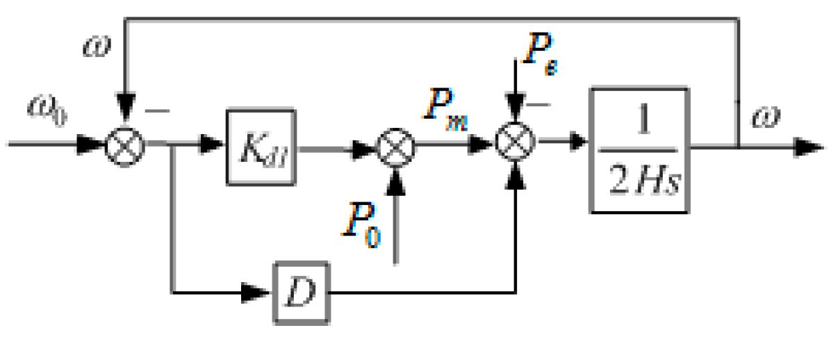
Figure 3 shows the simplified model of the SG turbine governing system. The swing equation of SG can be expressed as:
where Kd1 is the primary control coefficient of SG.
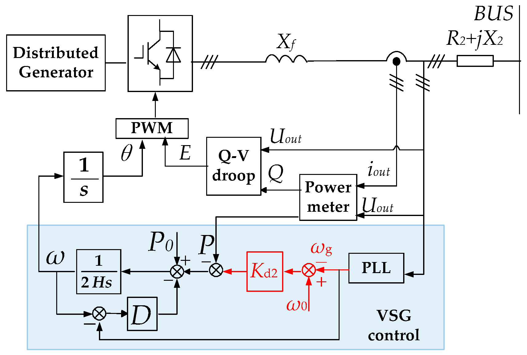
Figure 4 shows the basic control system of VSG2 which has the capability of primary frequency control. DGs employing this control can imitate the characteristics of SGs governing system.
The VSG controller can be represented as:
where Kd2 is the droop control coefficient of VSG2.
3. Mathematical Model of the Microgrids
This section focuses on the mathematic models of the two systems discussed in Section 2. The responses of frequency and output active power during a load step change are analyzed. The corresponding transfer functions are then deduced.
3.1. System 1: SG-Dominated Islanded Microgrid
For system 1, the output current of VSG can be derived as:
where impedance .
Thus the output apparent power of VSG can be conducted as follows:
where superscript “–” here indicates conjugate operation of the element, and impedance angle α = tan−1(X/R). Pe1 is the output active power. Qe1 is the output reactive power. It can be concluded from Equation (6) that:
Thus Equation (8) can be deduced as:
Let SE = EUsin(α − δ)/SnZ. SE is the synchronizing power coefficient. According to Equation (8),
Knowing that:
ωbus is the angular frequency of PCC. If Xf >> X1:
From (1) and (8)–(11), the transfer function for VSG can be obtained as:
The same derivation as (12) holds for SG:
From the law of conservation of energy:
Applying (12) and (13) to (14), we have:
and:
Applying (12) and (13) to (16):
Eliminating Δδ1 from Equations (9)–(11):
Applying (16) to (18):
Applying (12) and (13) to (19):
3.2. System 2: DG-Dominated Islanded Microgrid
For system 2, Equations (21) and (22) can be obtained by the same derivation:
Transfer function of output active power and frequency during a load transition can be constructed as follows:
Applying (21) and (22) to (23):
Applying (21) and (22) to (24):
4. Stability and Parameter Sensitivity Analysis
4.1. System 1: SG-Dominated Islanded Microgrid
The dynamics of system 1 is governed by the following three-order characteristic equation:
where:
Correspondingly, there are three eigenvalues.
For simplification, let:
Equation (27) can be transformed into:
According to the Cardan’s formula on cubic equation, we can get:
where:
Thus the roots of (27) can be deduced as:
where:
Parameters of system 1 are shown in Table 1. When Qref = 0 kVar, SE1 and SE2 can be calculated as 4.628 and 3.0865. And during the transient process, SE1 and SE2 are considered constant.
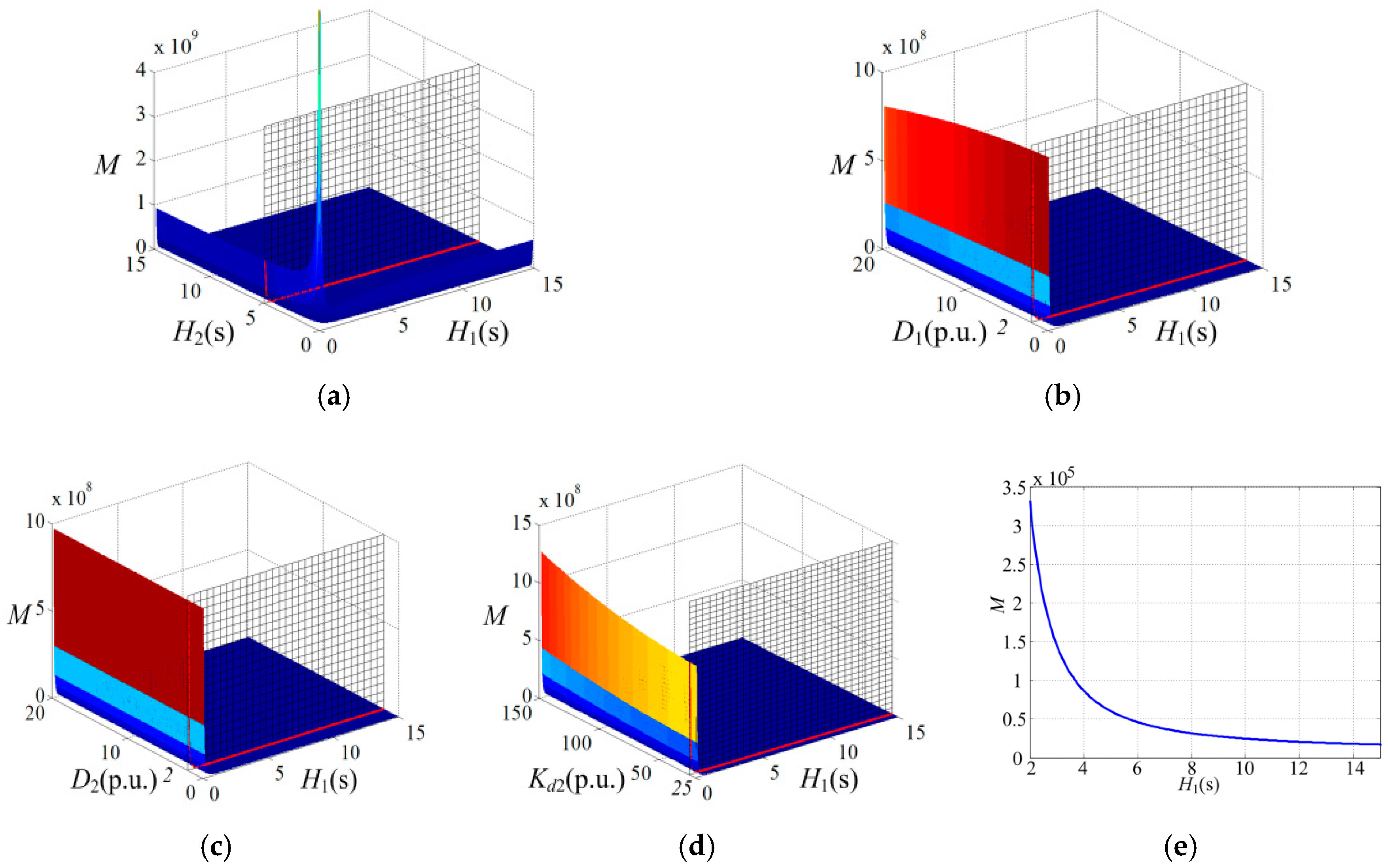
Figure 5 shows the variation range of M when H1, H2, D1, D2, Kd1 changes. H1 is the virtual inertia time constant of VSG. H2 is the virtual inertia time constant of SG. The “s” in brackets represent “second”, which is the unit of virtual inertia time constant, H. D1 is the damping coefficient of VSG. D2 is the damping coefficient of SG. Kd1 is the primary frequency regulation coefficient.
Therefore, if M > 0, according to (41) and (42), n1 and n2 are real and unequal. Then from (40), the imaginary parts of both x2 and x3 are none zero, which means there are two conjugate roots among the three eigenvalues. If M = 0, according to (41) and (42), n1 and n2 are real and equal. Then from (40), imaginary parts of both x2 and x3 are zero, which means the three eigenvalues are all real and x2 equal to x3. Under these circumstances, the real component of the conjugated eigenvalues can be calculated as:
It can be concluded from Figure 5 that, as the parameters H1, H2, D1, D2, Kd1 vary, M remains greater than or equal to 0, which makes the eigenvalues conjugate. When H2, D1, D2, Kd1 are chosen as Table 1, the cross-section curve of the surface on H1-M plane is presented in Figure 5e.
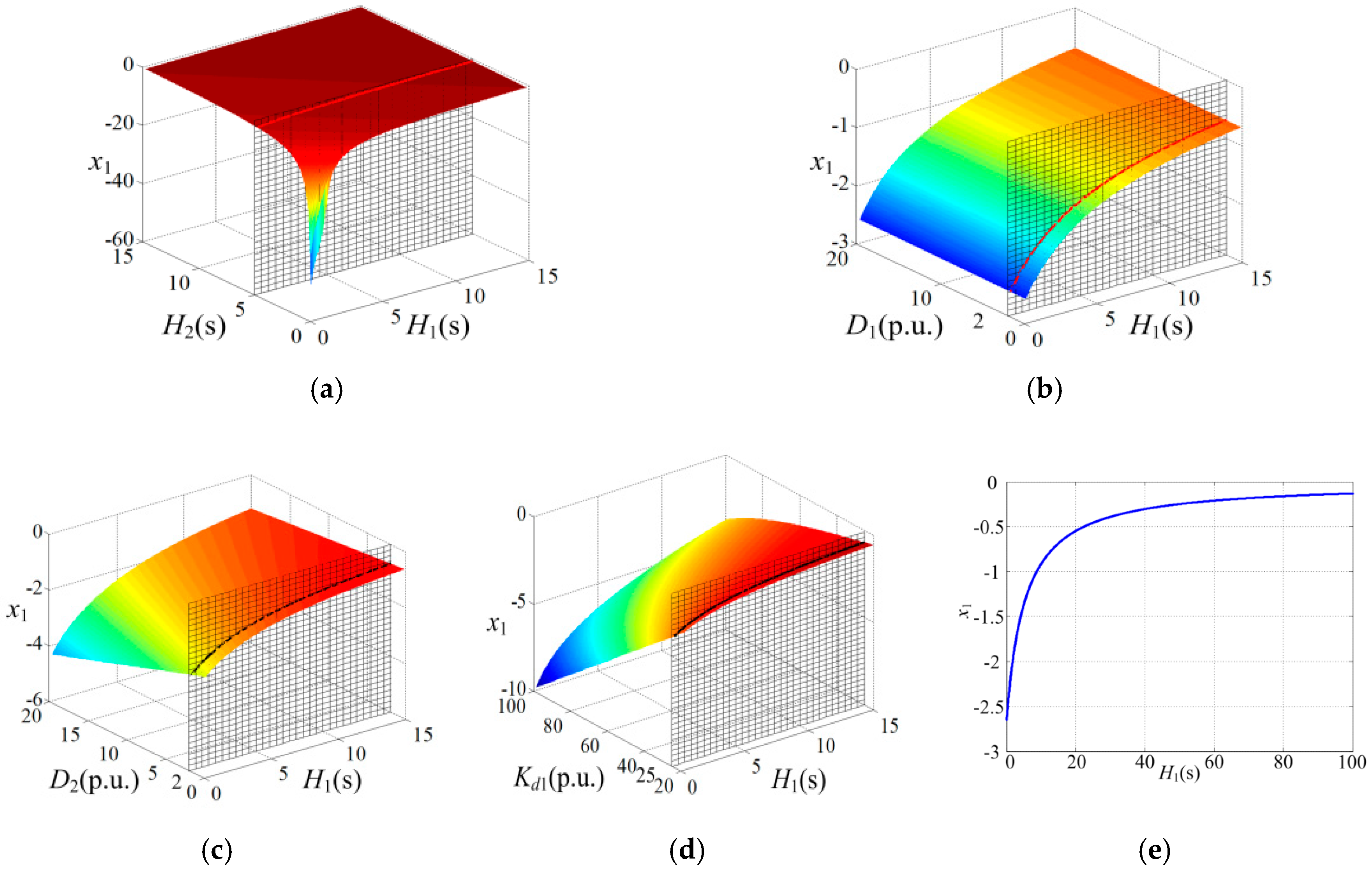
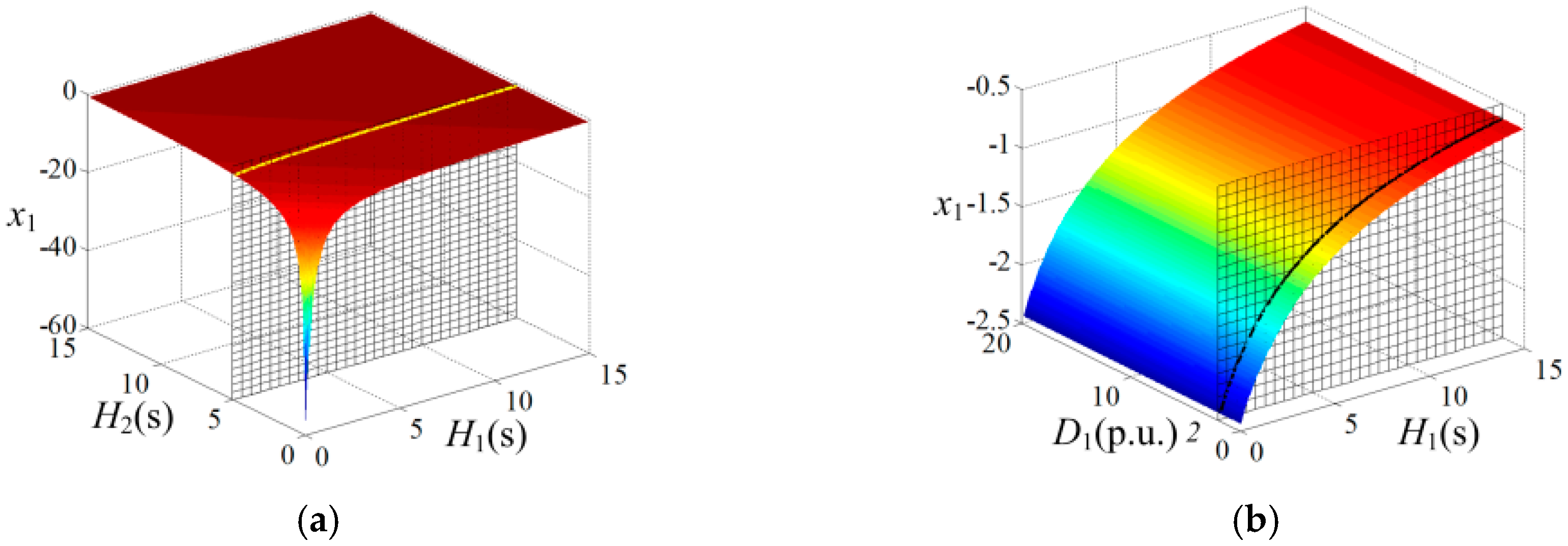
Figure 6 shows the variation of the real root, x1, when parameters H1, H2, D1, D2, Kd1 change. x1 keeps negative under these circumstances. The cross-section curve of the surface on H1-x1 plane when H2, D1, D2, Kd1 are chosen as Table 1 is presented in Figure 6e.
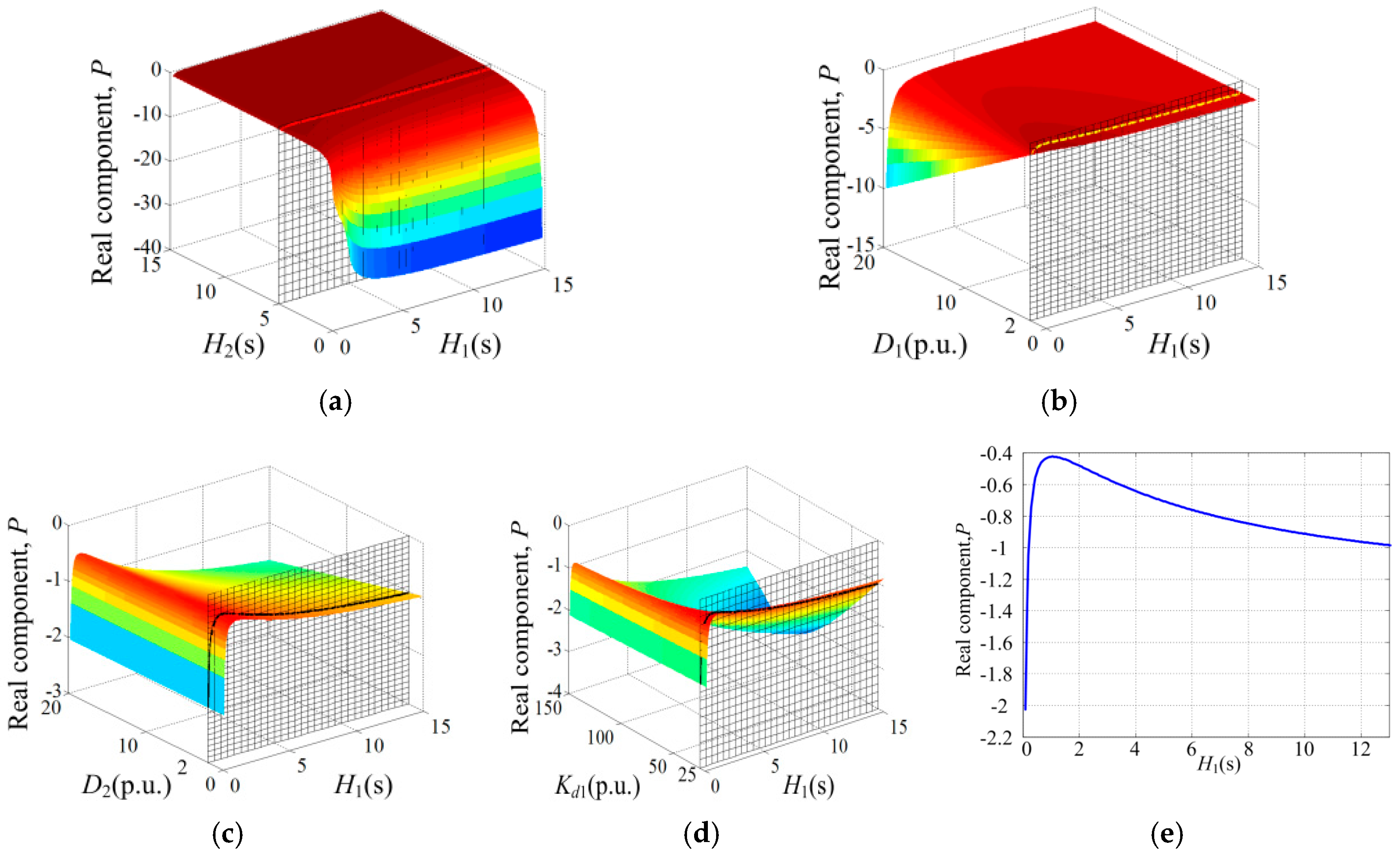
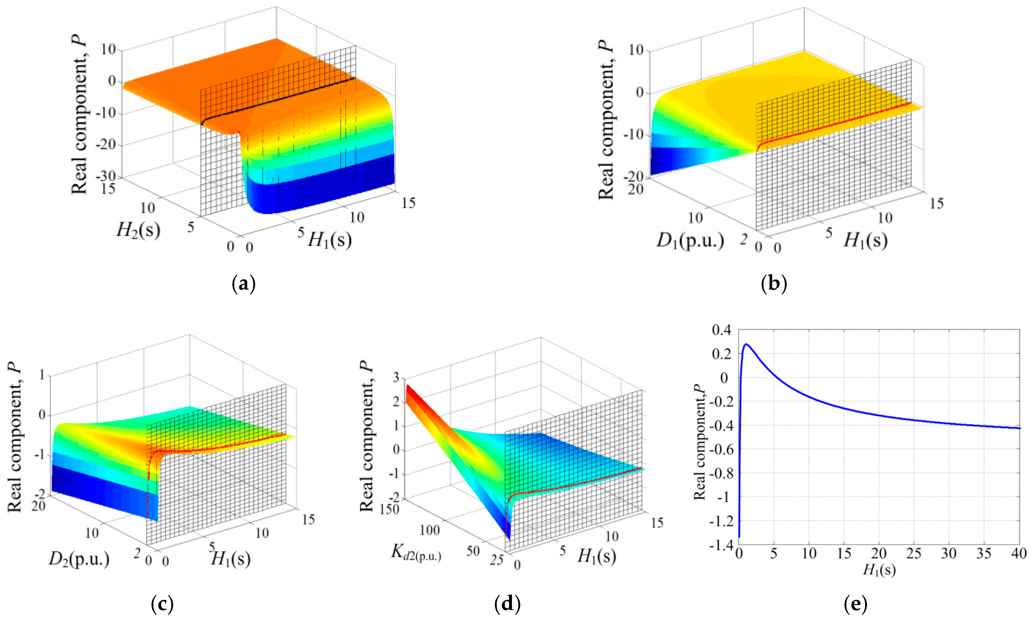
Figure 7 shows the variation of the real part of the conjugated eigenvalues, P, when parameters H1, H2, D1, D2, Kd1 change. It can be seen that P keeps negative under these circumstances, which makes the conjugate eigenvalues distribute on the left side of imaginary axis. Cross-section curve of the surface on H1-P plane when H2, D1, D2, Kd1 are chosen as Table 1 is presented in Figure 7e.
It can be concluded from Figure 5, Figure 6 and Figure 7 that the three eigenvalues will always distribute on the left side of the imaginary axis when the system parameters are varying in the reasonable range.
Figure 8 shows the root locus of system 1 when H1 changes. When H1 increases, the conjugate complex eigenvalues will approach the imaginary axis, which will result in deterioration of system stability. The eigenvalues will go away from imaginary axis when H1 keeps increasing.
The above analyses indicate that the system will keep stable.
4.2. System 2: DG-Dominated Islanded Microgrid
The dynamics of the system 2 is governed by the following three-order characteristic equation:
where:
The same derivation as (32)–(44) holds for system 2.
The parameters of system 2 are shown in Table 2. H1 is the virtual inertia time constant of VSG1. H2 is the virtual inertia time constant of VSG2. The “s” in brackets represent “second”, which is the unit of virtual inertia time constant, H. D1 is the damping coefficient of VSG1. D2 is the damping coefficient of VSG2. Kd2 is the primary frequency regulation coefficient.
Figure 9 shows the variation of M when parameters H1, H2, D1, D2, Kd2 change, from which we can see that M maintains positive. Figure 10 shows the variation of the real root, x1, which can also keeps positive under these circumstances. However as we can see in Figure 11, the real part of conjugate eigenvalues, P, will transcend the z = 0 axis, which means that the conjugate eigenvalues will distribute on the right side of the complex plane in some cases.
Similar conclusions can be drawn by the root locus shown in Figure 12. As H1 increases, the conjugate complex roots are approaching to the imaginary axis. Continuously increasing H1 will cause the roots crossing the imaginary axis and lead the system instable. If further increasing H1, the roots will go back to the left side of imaginary axis, in which cases the system can maintain stable again. This implies that there exists an unstable region for DG dominated islanded microgrid. The stable constraints can be calculated by the Routh Criterion.
According to the Routh Criterion, the system will remain stable if only the following inequality holds:
Thus, the stable region of H1 can be calculated as:
or:
where:
The stable constraints of H1 can be written as:
Figure 13 shows the range of Hmin and Hmax when H2, D1, D2 and Kd2 changes. According to Figure 13a, the increased D1 decreases both the upper limit Hmax and the lower limit Hmin. Larger D1 makes smaller instable regions. Figure 13b shows a similar influence of D2 as D1. It can also be seen from Figure 13c that both Hmax and Hmin are increased if H2 is raised. Increased H2 enlarges the unstable region. Figure 13d shows that larger Kd2 will decrease Hmin but increase Hmax, and thus makes a larger unstable region.
It can be seen from Figure 13 that the stable constraints are significantly affected by the system parameters. For example, increasing H1 from 0.06 (point A (5,0.06)) to 3 (point B (5,3)), and then to 9 (point C (5,9)), the system will go through an unstable region (Figure 13c). As a result, to maintain the stability of the microgrid, the constraints should be taken into account.
5. Simulation Analysis
The above ideas have been verified by simulations in this section. Simulation circuits of system 1 and system 2 are shown in Figure 14a,b. Simulations are carried out when load steps down to verify the theoretical analysis. The parameters of the two systems are shown in Table 1 and Table 2, respectively. The simulation was carried out in PSCAD/EMTDC. Switching frequency was set at 10 kHz and solution time step was set at 1 μs.
5.1. System Performance Simulation
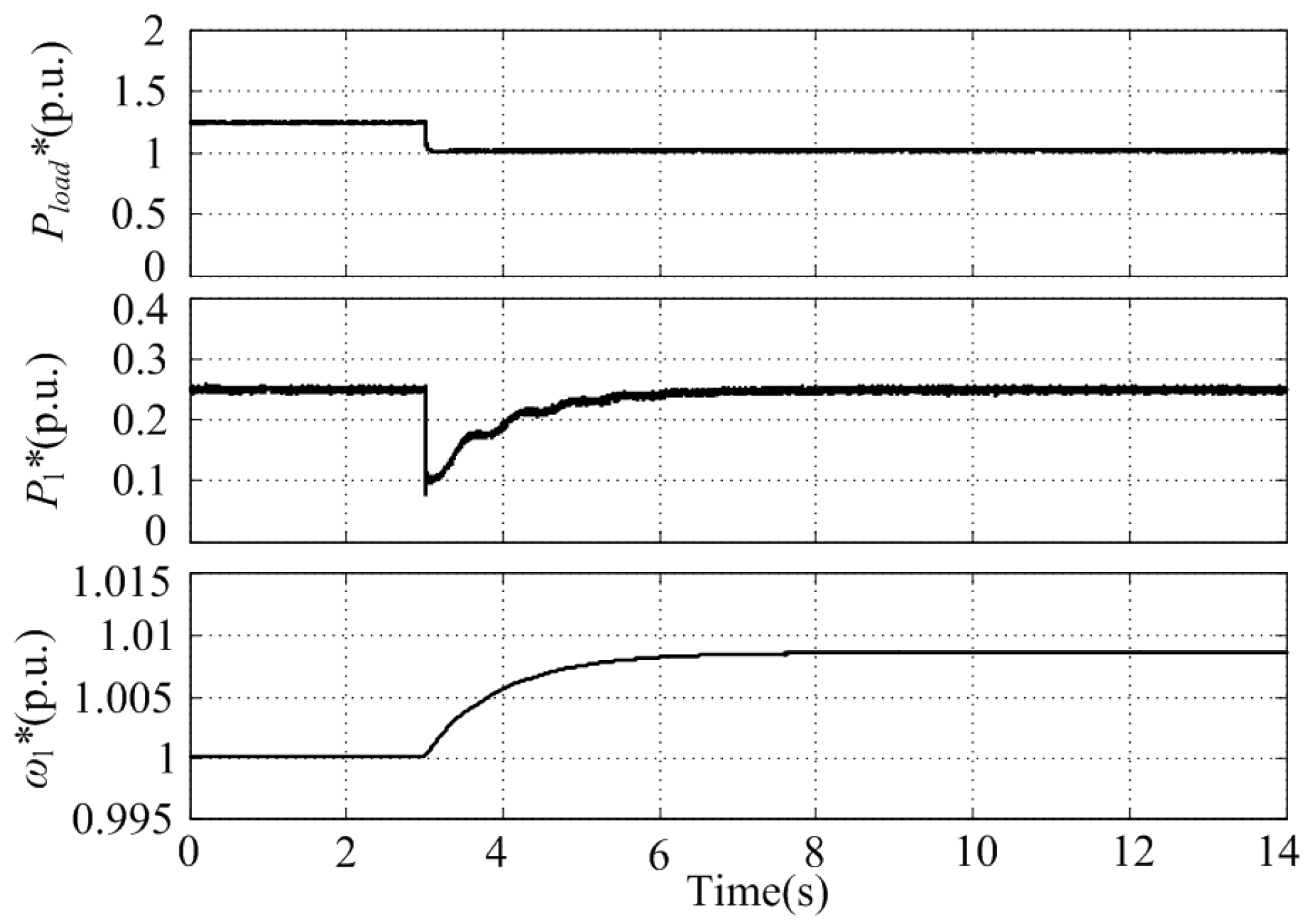
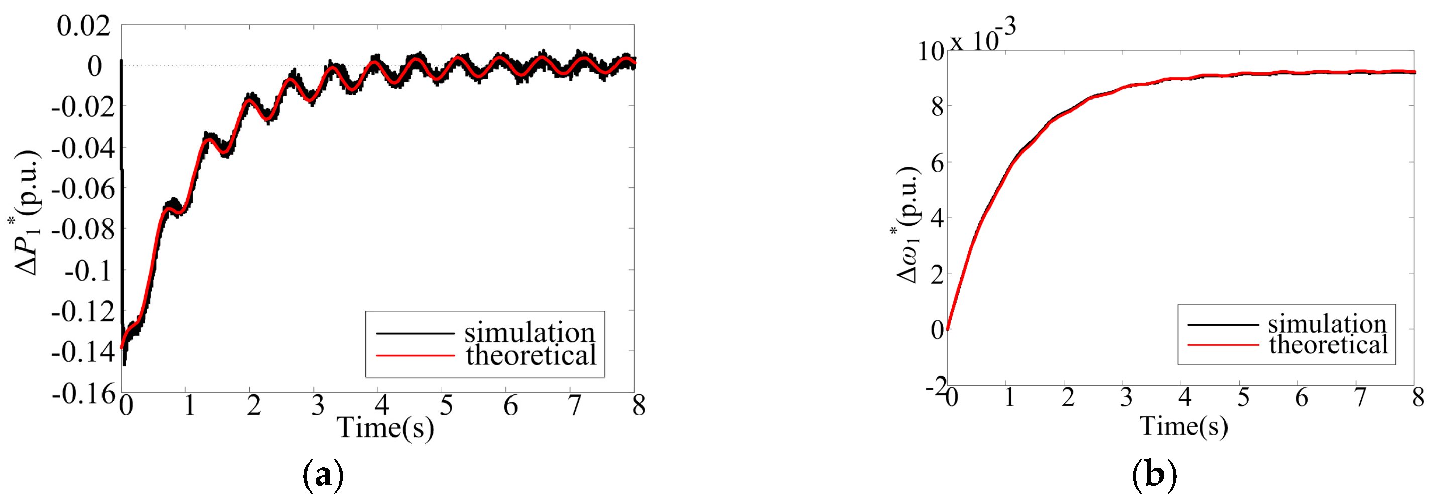
In Figure 15 and Figure 16, the two systems were initially working in steady state. When load stepped down from 1.25 p.u. to 1 p.u. at t = 3 s, the output powers of VSG in system 1 and VSG1 in system 2 decreased and the frequencies increased correspondingly. Moreover, we could see from Figure 17 and Figure 18 that during the transient process, the simulation results (black lines) coincided with corresponding theoretical results (red lines). These results verify the small-signal models of the two systems. And it can be noticed that the SG-dominated system shows smaller fluctuations in dynamical behaviors.
5.2. Stability of the Two Systems
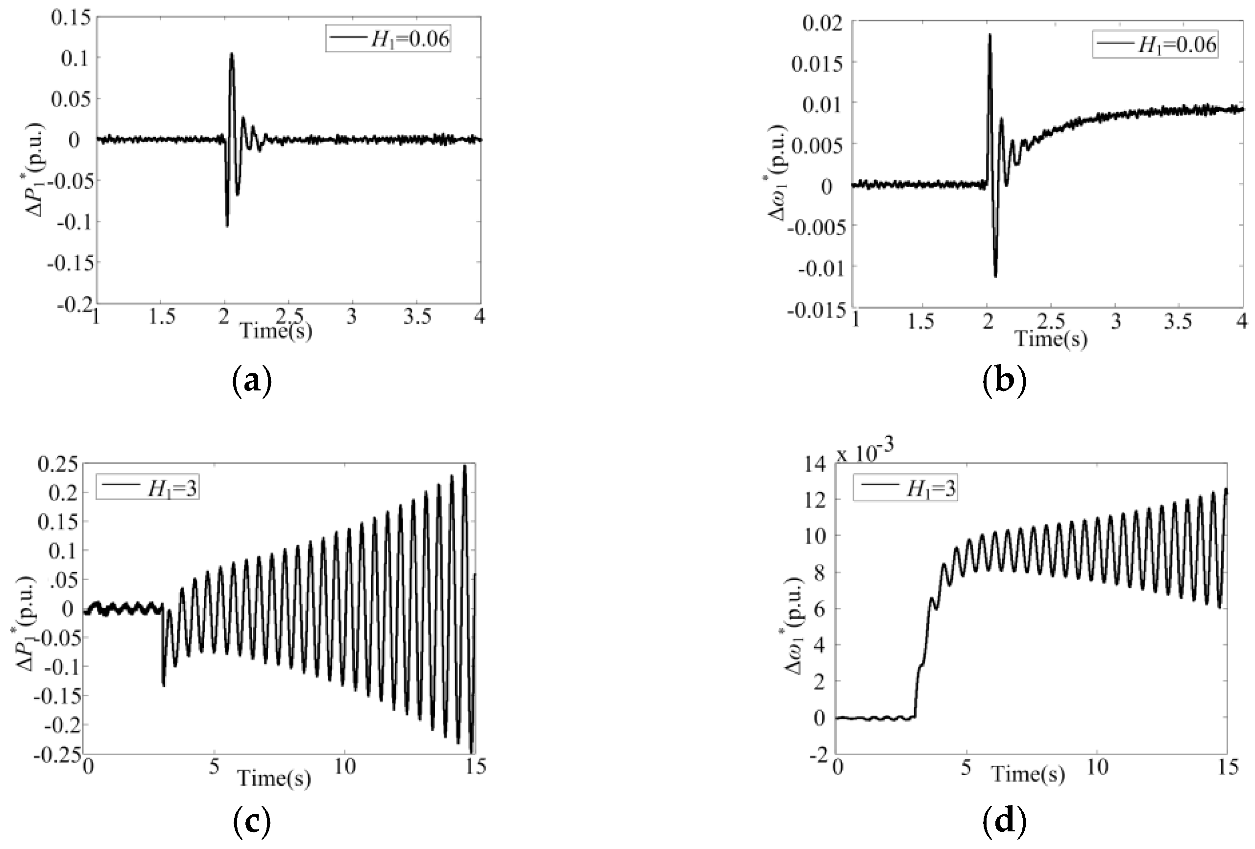
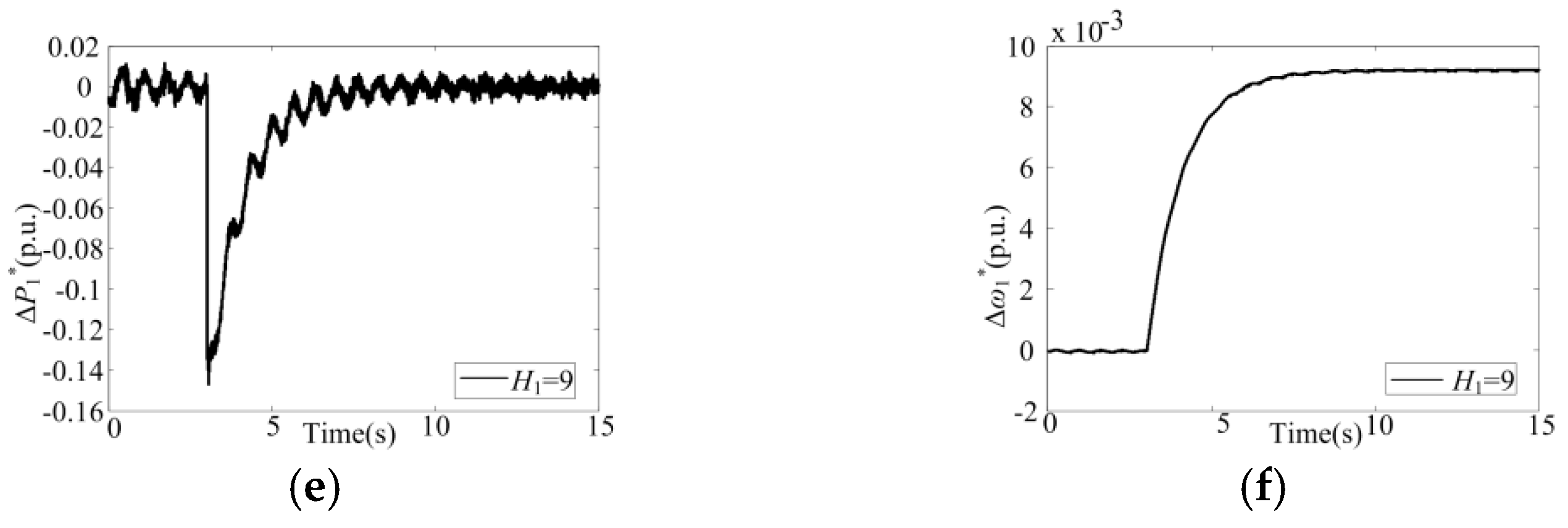
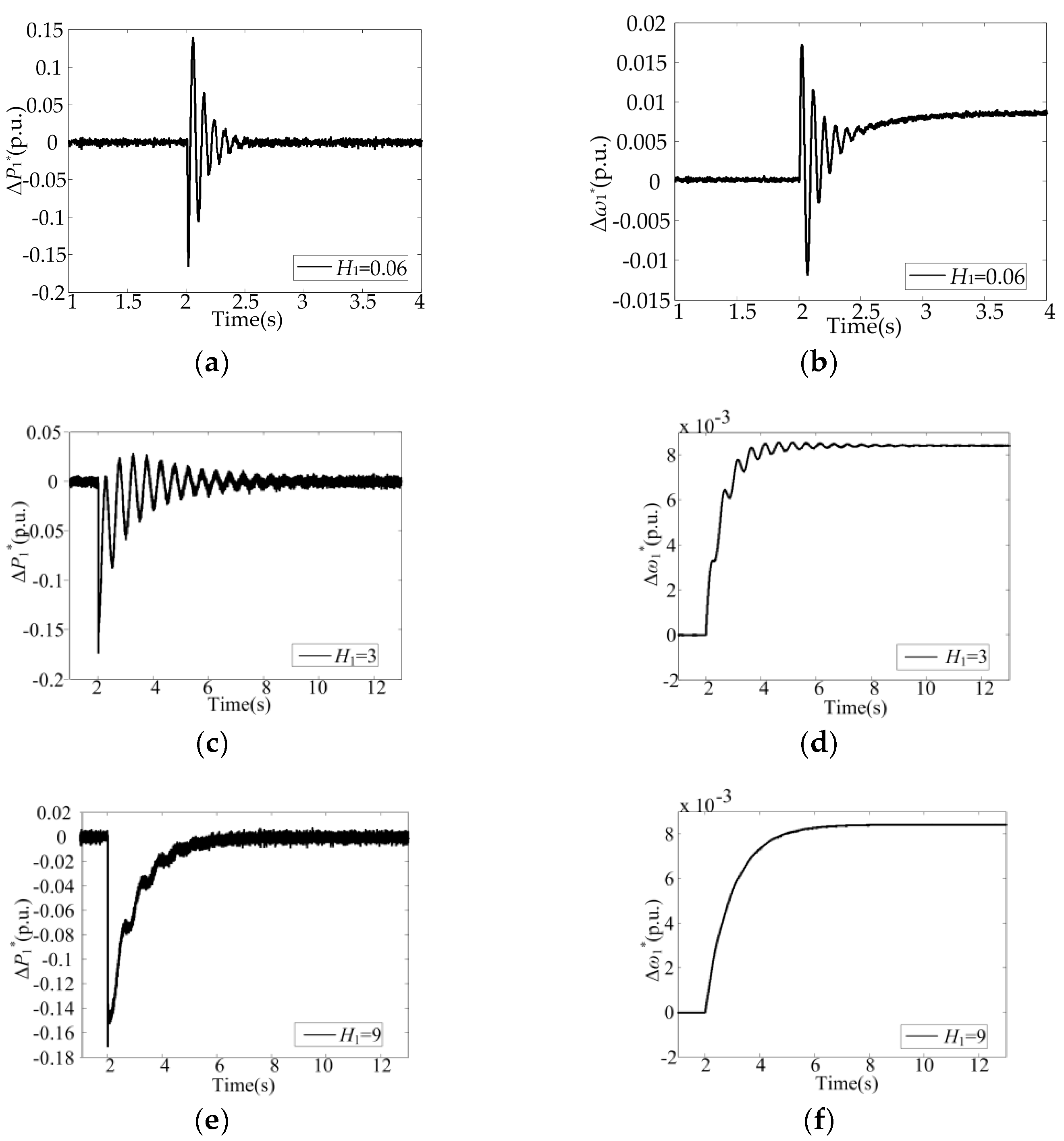
When the virtual inertia time constant H takes different values, the comparison of the two systems is carried out in this part. The load steps at t = 2 s, and other parameters are set up as shown in Table 1 and Table 2. The three values of H1 correspond to the point A, B and C shown in Figure 13c, respectively. When adopting different H1, the transient responses of the output active power deviation and the frequency deviation of VSG in system 1 and VSG1 in system 2 are shown in Figure 19 and Figure 20.
It can be seen from Figure 19 that the virtual inertia H1 influences the dynamical behaviors but has no affect on the final stable state. However, completely different results for system 2 are shown in Figure 20. As shown in Figure 20a,b, if operating at point A, where H1 = 0.06, the system remains stable when small load disturbance occurs. In Figure 20c,d increased H1 will cause the system to be unstable. While, as shown in Figure 20e,f, the system will remain stable if H1 increases further. Compared to system 1, there is a slight fluctuation under steady state for system 2. The simulation results verify that virtual inertia H1 shows different affects on the two systems. System 1 faces severer stability issues. And the inappropriate H1 will cause the system to be unstable when facing small disturbances.
6. Conclusions
This paper identifies the unstable region of islanded AC microgrids through detailed transient stability analysis.
Firstly, this paper established the simplified models of two kinds of islanded AC microgrids, SG-dominated islanded microgrids and DG-dominated islanded microgrid. Then, based on the models, it was noted that compared to the SG-dominated islanded microgrids, there were potential stability issues for DG-dominated islanded microgrids. Mathematical calculation methods were used to study the unstable region, and the influences of key parameters on unstable constraints were discussed. Finally, detailed simulation results verified the theoretical analysis. The identified unstable region provided an important basis for the parameter tuning of VSG operating in an island microgrid.
Author Contributions
C.Y. drove the whole theoretical analysis and simulation work. P.X. contributed the theoretical analysis and wrote the paper. D.Y. performed the simulations. And X.X. guided the whole work and pointed out the direction of the research.
Conflicts of Interest
The authors declare no conflict of interest.
References
- China National Energy Administration. National Energy Board News Conference to Introduce the Energy Situation in the First Half of the Year. 2017. Available online: http://www.nea.gov.cn/2017-07/21/c_136461811.htm (accessed on 15 November 2017). (In Chinese)
- Bevrani, H.; Ise, T.; Miura, Y. Virtual synchronous generators: A survey and new perspectives. Int. J. Electr. Power Energy Syst. 2014, 54, 244–254. [Google Scholar] [CrossRef]
- Majumder, R. Some Aspects of Stability in Microgrids. IEEE Trans. Power Syst. 2013, 28, 3243–3252. [Google Scholar] [CrossRef]
- Majumder, R.; Ghosh, A.; Ledwich, G.; Zare, F. Power Sharing and Stability Enhancement of an Autonomous Microgrid with Inertial and Non-inertial DGs with DSTATCOM. In Proceedings of the IEEE International Conference on Power Systems, Kharagpur, India, 27–29 December 2009; pp. 1–6. [Google Scholar]
- Soni, N.; Doolla, S.; Chandorkar, M.C. Improvement of Transient Response in Microgrids Using Virtual Inertia. IEEE Trans. Power Deliv. 2013, 28, 1830–1838. [Google Scholar] [CrossRef]
- Alipoor, J.; Miura, Y.; Ise, T. Power System Stabilization Using Virtual Synchronous Generator with Alternating Moment of Inertia. IEEE J. Emerg. Sel. Top. Power Electron. 2015, 3, 451–458. [Google Scholar] [CrossRef]
- Zhong, Q.; Weiss, G. Synchronverters: Inverters That Mimic Synchronous Generators. IEEE Trans. Ind. Electron. 2011, 58, 1259–1267. [Google Scholar] [CrossRef]
- Wu, H.; Ruan, X.; Yang, D.; Chen, X.; Zhao, W.; Lv, Z.; Zhong, Q.-C. Small-Signal Modeling and Parameters Design for Virtual Synchronous Generators. IEEE Trans. Ind. Electron. 2016, 63, 4292–4303. [Google Scholar] [CrossRef]
- Alipoor, J.; Miura, Y.; Ise, T. Evaluation of Virtual Synchronous Generator (VSG) Operation under Different Voltage Sag Conditions. In Proceedings of the IEEJ Conference on Power Technology and Power Systems, Tokyo, Japan, 6–7 August 2012; pp. 41–46. [Google Scholar]
- Torres, L.M.A.; Lopes, L.A.C.; Moran, T.L.A.; Espinoza, C.J.R. Self-tuning virtual synchronous machine: A control strategy for energy storage systems to support dynamic frequency control. IEEE Trans. Energy Convers. 2014, 29, 833–840. [Google Scholar] [CrossRef]
- Hirase, Y.; Noro, O.; Yoshimura, E.; Nakagawa, H.; Sakimoto, K.; Shindo, Y. Virtual synchronous generator control with double decoupled synchronous reference frame for single-phase inverter. IEEJ J. Ind. Appl. 2015, 4, 143–151. [Google Scholar] [CrossRef]
- Sakimoto, K.; Miura, Y.; Ise, T. Stabilization of a power system with a distributed generator by a virtual synchronous generator function. In Proceedings of the IEEE 8th International Conference on Power Electronics and ECCE Asia, Shilla Jeju, Korea, 30 May–3 June 2011; pp. 1498–1505. [Google Scholar]
- Shintai, T.; Miura, Y.; Ise, T. Reactive power control for load sharing with virtual synchronous generator control. In Proceedings of the 7th International Power Electronics and Motion Control Conference (IPEMC), Harbin, China, 2–5 June 2012; pp. 846–853. [Google Scholar]
- Shintai, T.; Miura, Y.; Ise, T. Oscillation damping of a distributed generator using a virtual synchronous generator. IEEE Trans. Power Deliv. 2014, 29, 668–676. [Google Scholar] [CrossRef]
- China Southern Power Grid. Network Operation of the First Virtual Synchronous Machine System of China Southern Power Grid. 2017. Available online: http://www.csg.cn/xwzx/2017/gsyw/201702/t20170222_151669.html (accessed on 21 February 2017). (In Chinese).
- China Energy News. Virtual Synchronous Generator Demonstration Project Puts into Operation. 2017. Available online: http://paper.people.com.cn/zgnyb/html/2017-01/02/content_1740630.htm (accessed on 2 January 2017). (In Chinese).
- Liu, J.; Miura, Y.; Ise, T. Comparison of Dynamic Characteristics between Virtual Synchronous Generator and Droop Control in Inverter-Based Distributed Generators. IEEE Trans. Power Electron. 2016, 31, 3600–3611. [Google Scholar] [CrossRef]
- Yuan, C.; Liu, C.; Zhang, X.; Zhao, T.; Xiao, X.; Tang, N. Comparison of Dynamic Characteristics between Virtual Synchronous Machines Adopting Different Active Power Droop Controls. J. Power Electron. 2017, 17, 766–776. [Google Scholar] [CrossRef]
- Alipoor, J.; Miura, Y.; Ise, T. Distributed generation grid integration using virtual synchronous generator with adoptive virtual inertia. In Proceedings of the Energy Conversion Congress and Exposition, Denver, CO, USA, 15–19 September 2013; pp. 4546–4552. [Google Scholar]
- Fan, W.; Yan, X.; Hua, T. Adaptive parameter control strategy of VSG for improving system transient stability. In Proceedings of the IEEE 3rd International Future Energy Electronics Conference and ECCE Asia, Kaohsiung, Taiwan, 3–7 June 2017; pp. 2053–2058. [Google Scholar]
- Li, D.; Zhu, Q.; Lin, S.; Bian, X.Y. A Self-Adaptive Inertia and Damping Combination Control of VSG to Support Frequency Stability. IEEE Trans. Energy Convers. 2017, 32, 397–398. [Google Scholar] [CrossRef]
- Zheng, T.; Chen, L.; Wang, R.; Li, C.; Mei, S. Adaptive damping control strategy of virtual synchronous generator for frequency oscillation suppression. In Proceedings of the 12th IET International Conference on AC and DC Power Transmission (ACDC 2016), Beijing, China, 28–29 May 2016. [Google Scholar]
Figure 1.
A typical microgrid with VSG: (a) System 1: synchronous generator (SG)-dominated islanded microgrid; (b) System 2: distributed generator (DG)-dominated islanded microgrid.
Figure 1.
A typical microgrid with VSG: (a) System 1: synchronous generator (SG)-dominated islanded microgrid; (b) System 2: distributed generator (DG)-dominated islanded microgrid.
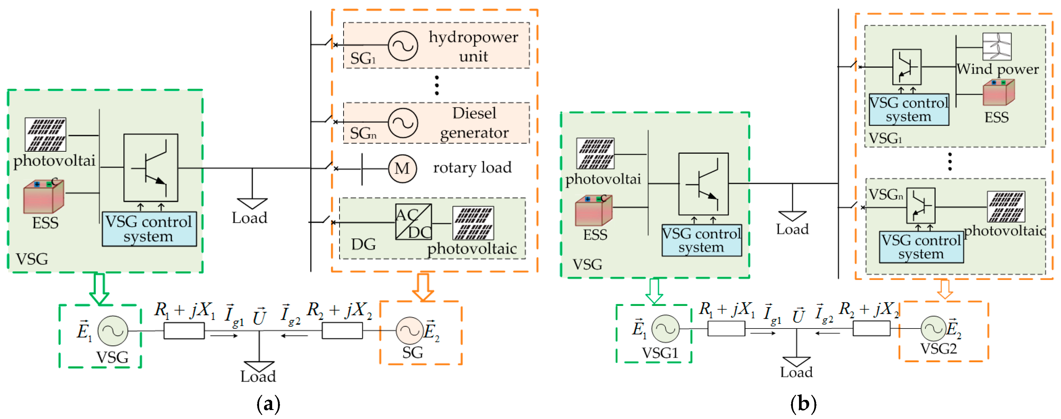
Figure 2.
Basic control systems of VSG and VSG1 without primary frequency control.
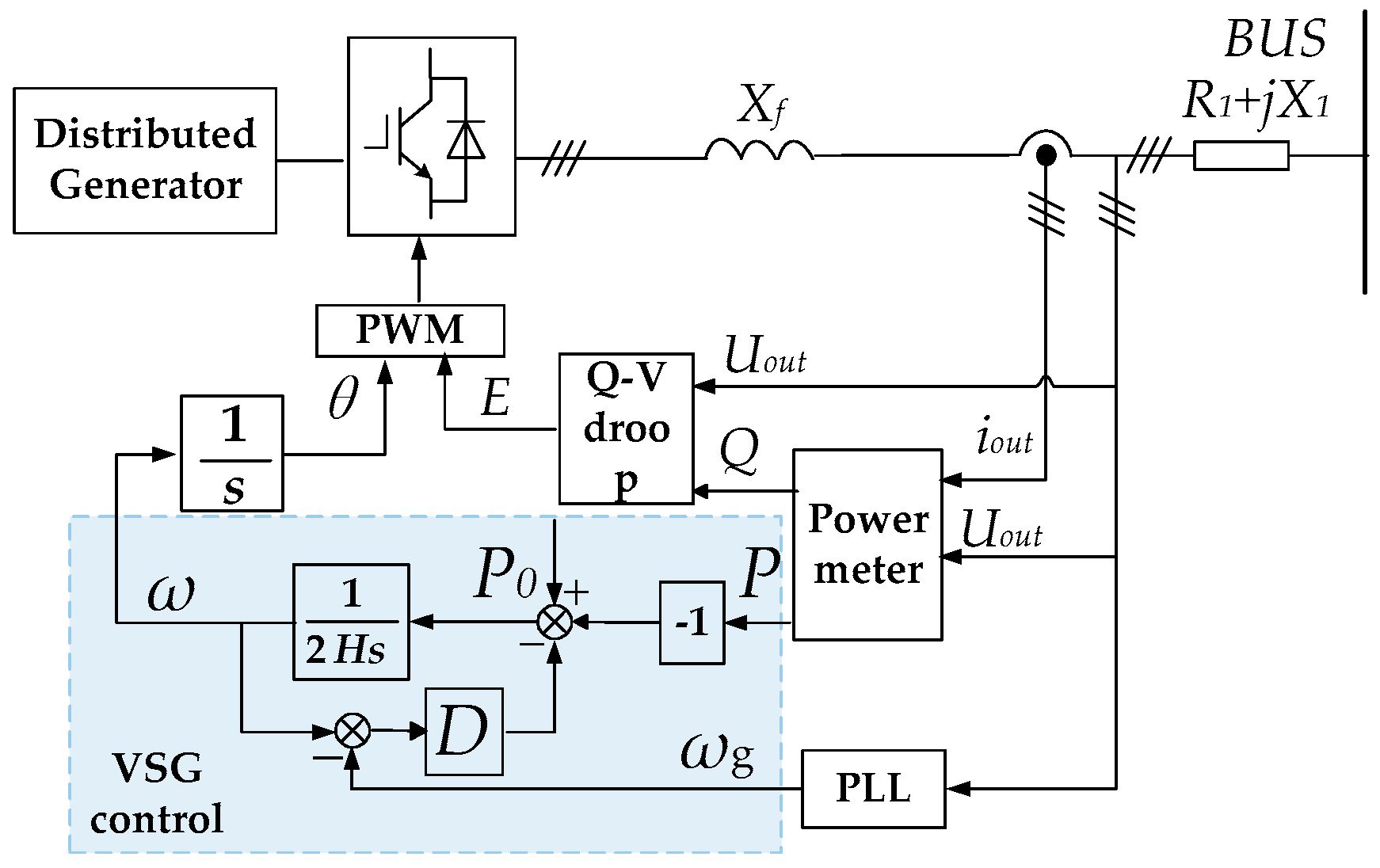
Figure 3.
Simplified model of the SG turbine governing system.

Figure 4.
Basic control systems of VSG2 which has the capability of primary frequency control.

Figure 5.
The variation range of M: (a) H1 and H2 vary from 0 to 15; (b) H1 varies from 0 to 15, D1 varies from 0 to 20; (c) H1 varies from 0 to 15, D2 vary from 0 to 20; (d) H1 varies from 0 to 15, Kd1 varies from 20 to 100; (e) Cross-section of M.
Figure 5.
The variation range of M: (a) H1 and H2 vary from 0 to 15; (b) H1 varies from 0 to 15, D1 varies from 0 to 20; (c) H1 varies from 0 to 15, D2 vary from 0 to 20; (d) H1 varies from 0 to 15, Kd1 varies from 20 to 100; (e) Cross-section of M.
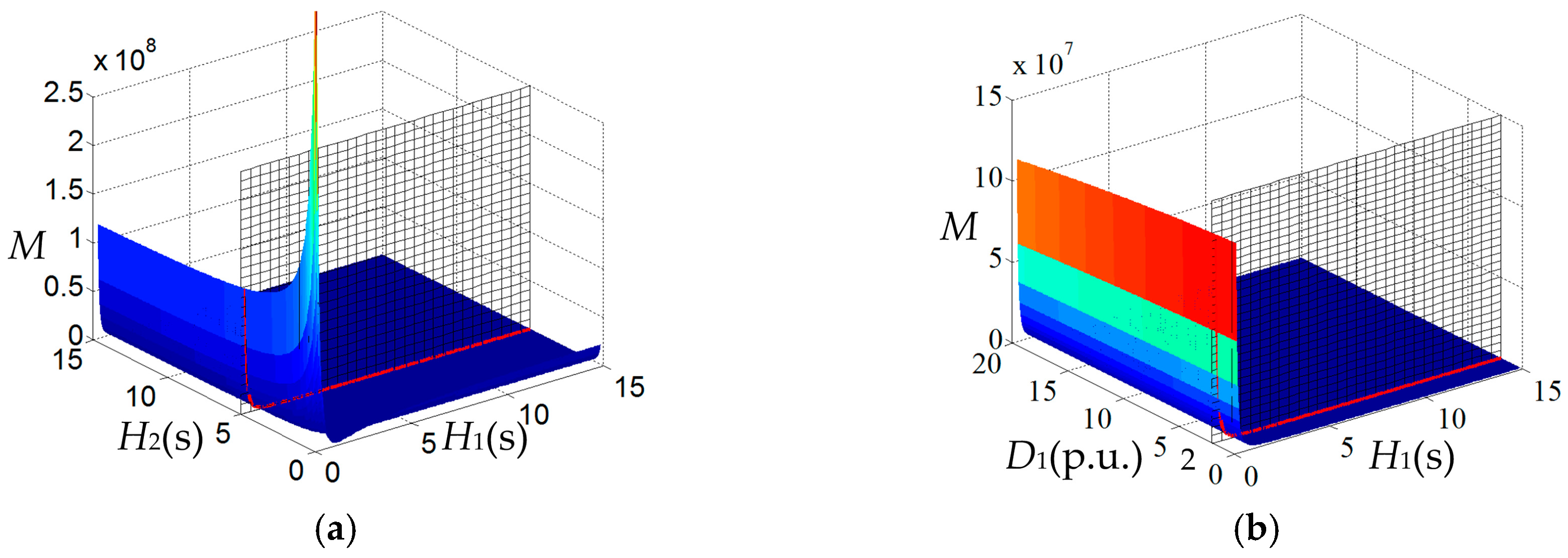
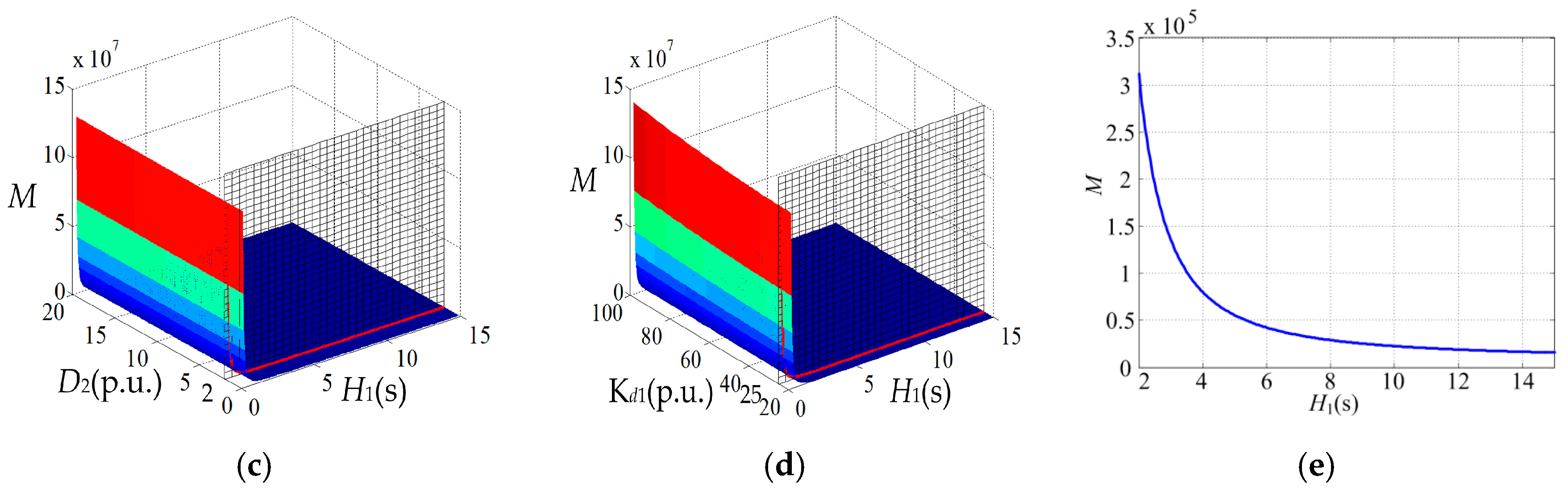
Figure 6.
The variation range of x1: (a) H1 and H2 vary from 0 to 15; (b) H1 varies from 0 to 15, D1 varies from 0 to 20; (c) H1 varies from 0 to 15, D2 vary from 0 to 20; (d) H1 varies from 0 to 15, Kd1 varies from 20 to 100; (e) Cross-section of x1.
Figure 6.
The variation range of x1: (a) H1 and H2 vary from 0 to 15; (b) H1 varies from 0 to 15, D1 varies from 0 to 20; (c) H1 varies from 0 to 15, D2 vary from 0 to 20; (d) H1 varies from 0 to 15, Kd1 varies from 20 to 100; (e) Cross-section of x1.

Figure 7.
The variation range of P: (a) H1 and H2 vary from 0 to 15; (b) H1 varies from 0 to 15, D1 varies from 0 to 20; (c) H1 varies from 0 to 15, D2 vary from 0 to 20; (d) H1 varies from 0 to 15, Kd1 varies from 20 to 100; (e) Cross-section of P.
Figure 7.
The variation range of P: (a) H1 and H2 vary from 0 to 15; (b) H1 varies from 0 to 15, D1 varies from 0 to 20; (c) H1 varies from 0 to 15, D2 vary from 0 to 20; (d) H1 varies from 0 to 15, Kd1 varies from 20 to 100; (e) Cross-section of P.

Figure 8.
Root locus of system 1 when H1 changes.
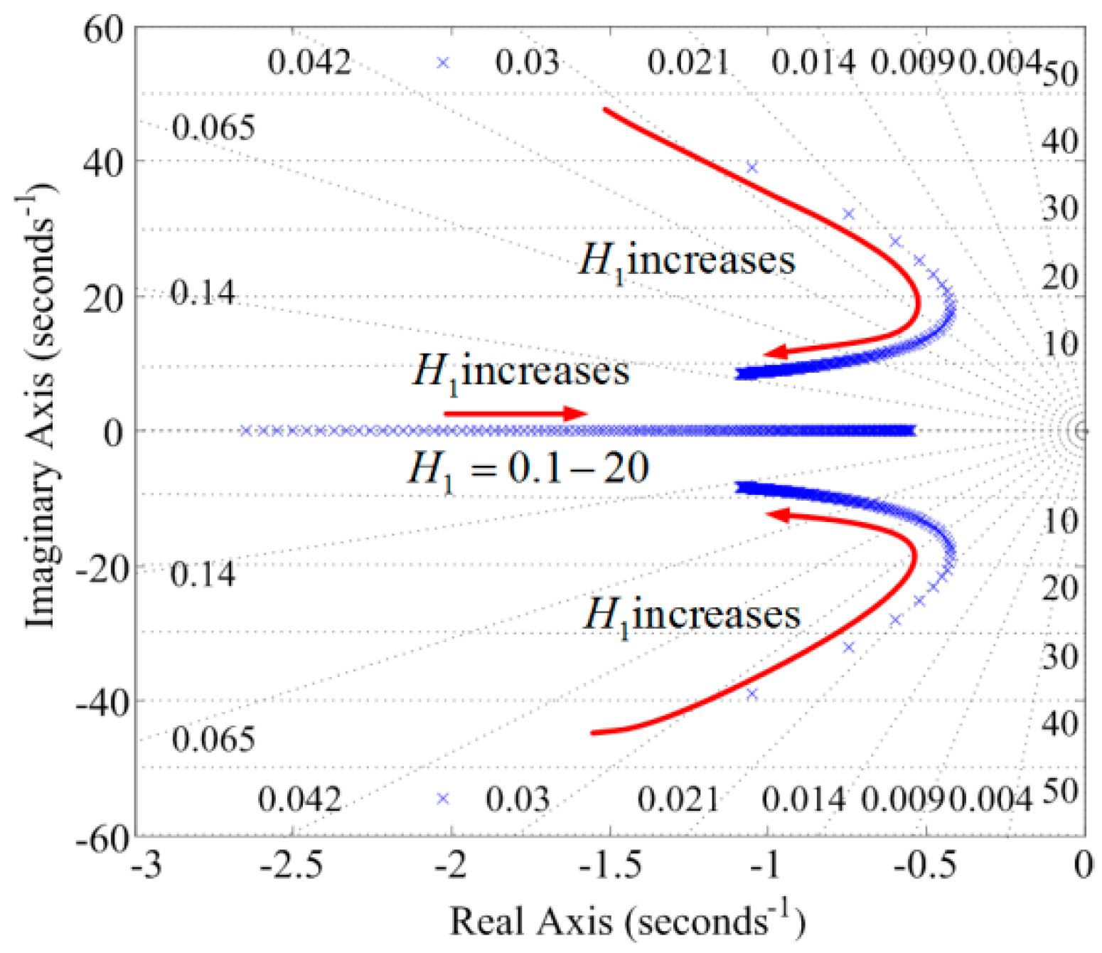
Figure 9.
The variation range of M: (a) H1 and H2 vary from 0 to 15; (b) H1 varies from 0 to 15, D1 varies from 0 to 20; (c) H1 varies from 0 to 15, D2 vary from 0 to 20; (d) H1 varies from 0 to 15, Kd1 varies from 20 to 150; (e) Cross-section of M.
Figure 9.
The variation range of M: (a) H1 and H2 vary from 0 to 15; (b) H1 varies from 0 to 15, D1 varies from 0 to 20; (c) H1 varies from 0 to 15, D2 vary from 0 to 20; (d) H1 varies from 0 to 15, Kd1 varies from 20 to 150; (e) Cross-section of M.

Figure 10.
The variation range of x1: (a) H1 and H2 vary from 0 to 15; (b) H1 varies from 0 to 15, D1 varies from 0 to 20; (c) H1 varies from 0 to 15, D2 vary from 0 to 20; (d) H1 varies from 0 to 15, Kd1 varies from 20 to 150; (e) Cross-section of x1.
Figure 10.
The variation range of x1: (a) H1 and H2 vary from 0 to 15; (b) H1 varies from 0 to 15, D1 varies from 0 to 20; (c) H1 varies from 0 to 15, D2 vary from 0 to 20; (d) H1 varies from 0 to 15, Kd1 varies from 20 to 150; (e) Cross-section of x1.

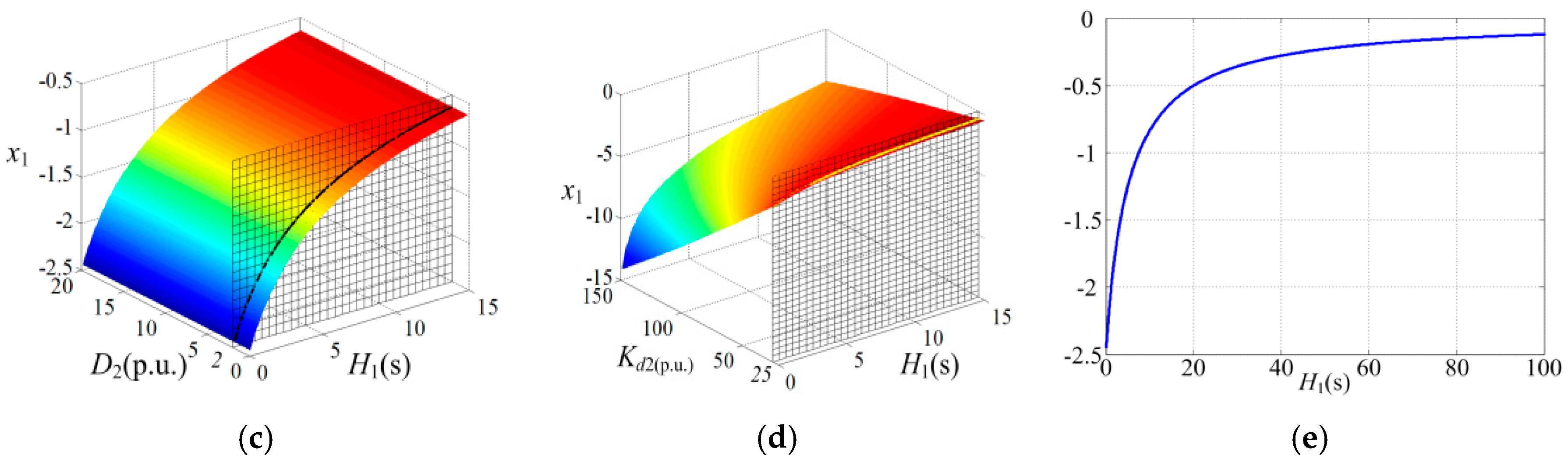
Figure 11.
The variation range of P: (a) H1 and H2 vary from 0 to 15; (b) H1 varies from 0 to 15, D1 varies from 0 to 20; (c) H1 varies from 0 to 15, D2 vary from 0 to 20; (d) H1 varies from 0 to 15, Kd1 varies from 20 to 150; (e) Cross-section of P.
Figure 11.
The variation range of P: (a) H1 and H2 vary from 0 to 15; (b) H1 varies from 0 to 15, D1 varies from 0 to 20; (c) H1 varies from 0 to 15, D2 vary from 0 to 20; (d) H1 varies from 0 to 15, Kd1 varies from 20 to 150; (e) Cross-section of P.

Figure 12.
Root locus of system 2 when H1 changes.
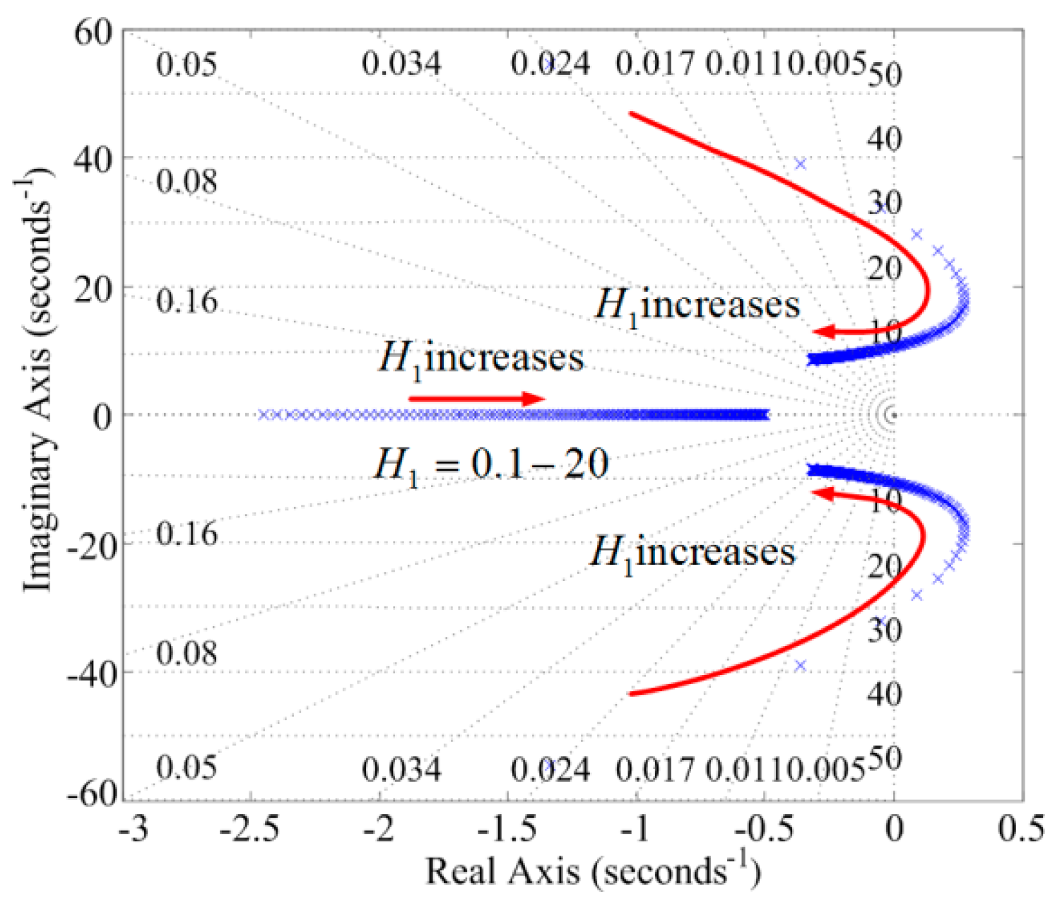
Figure 13.
The unstable constraints of H1: (a) The stable constraints when D1 changes; (b) The stable constraints when D2 changes; (c) The stable constraints when H2 changes; (d) The stable constraints when Kd2 changes.
Figure 13.
The unstable constraints of H1: (a) The stable constraints when D1 changes; (b) The stable constraints when D2 changes; (c) The stable constraints when H2 changes; (d) The stable constraints when Kd2 changes.
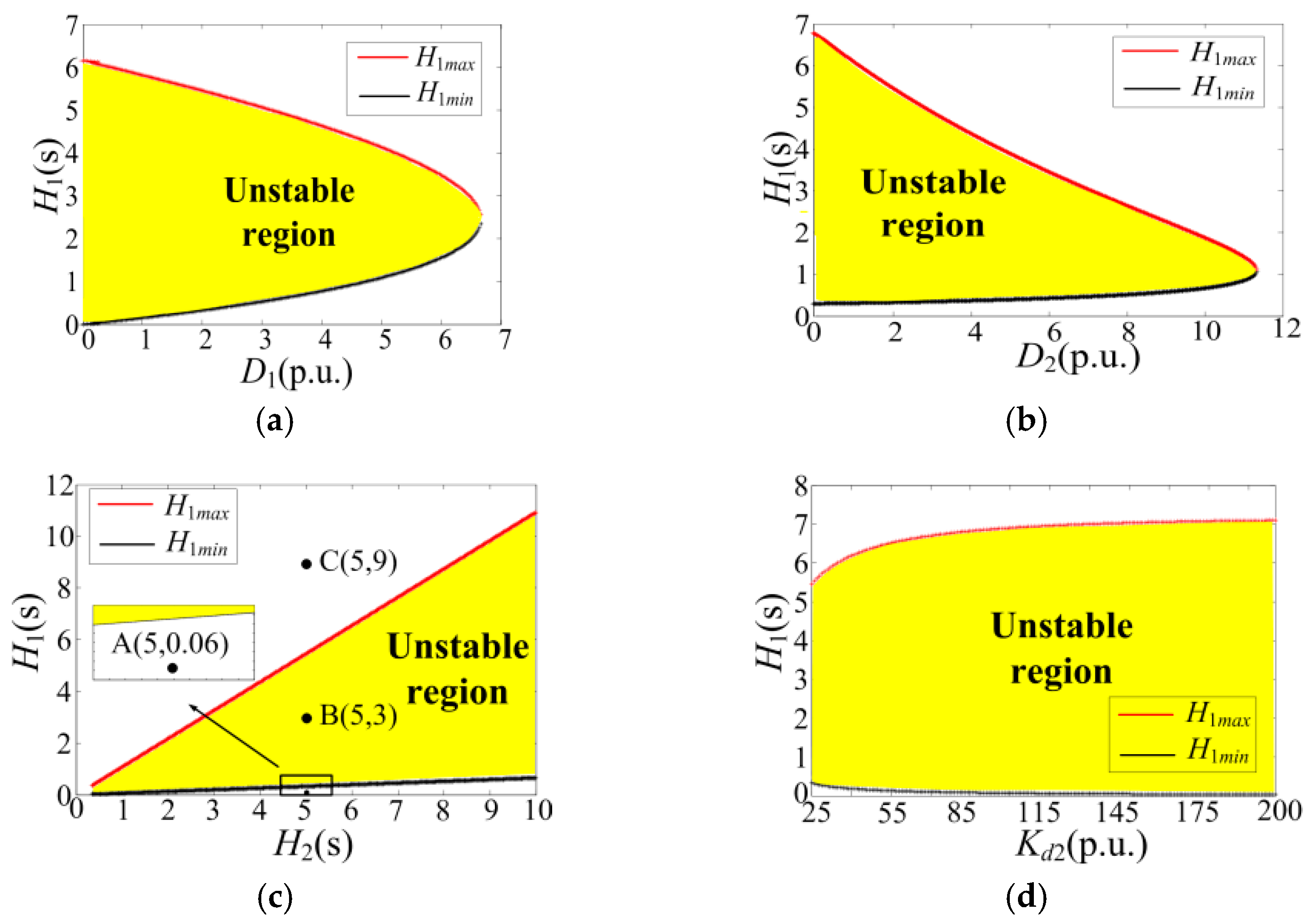
Figure 14.
Schematic diagram of islanded microgrid simulation system (a) System 1; (b) System 2.
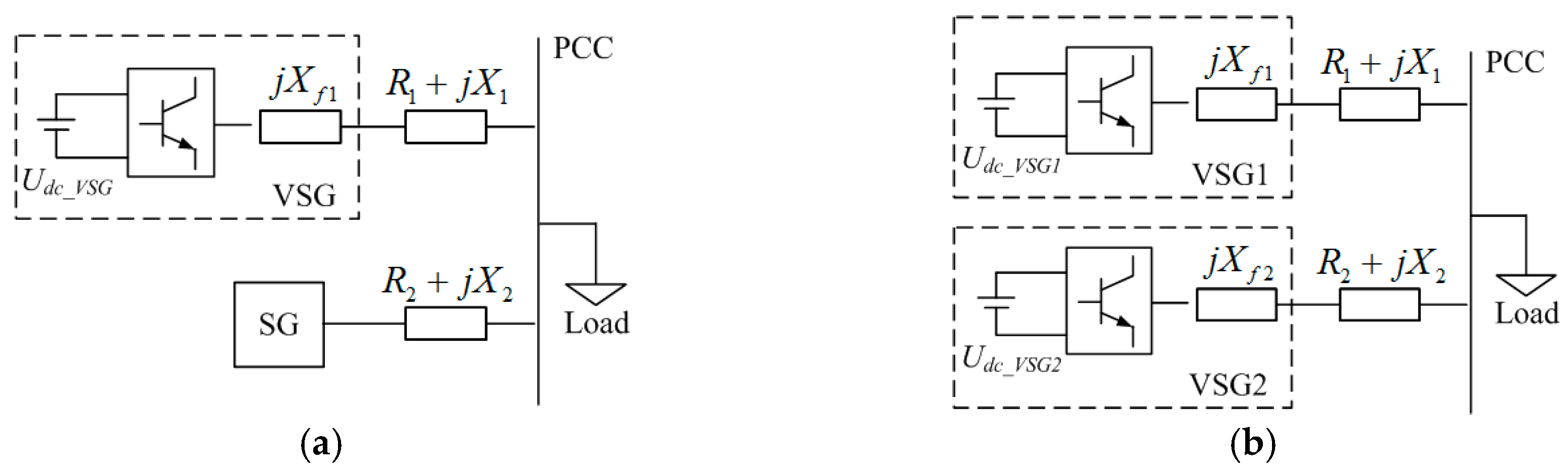
Figure 15.
Transient response for system 1.

Figure 16.
Transient response for system 2.
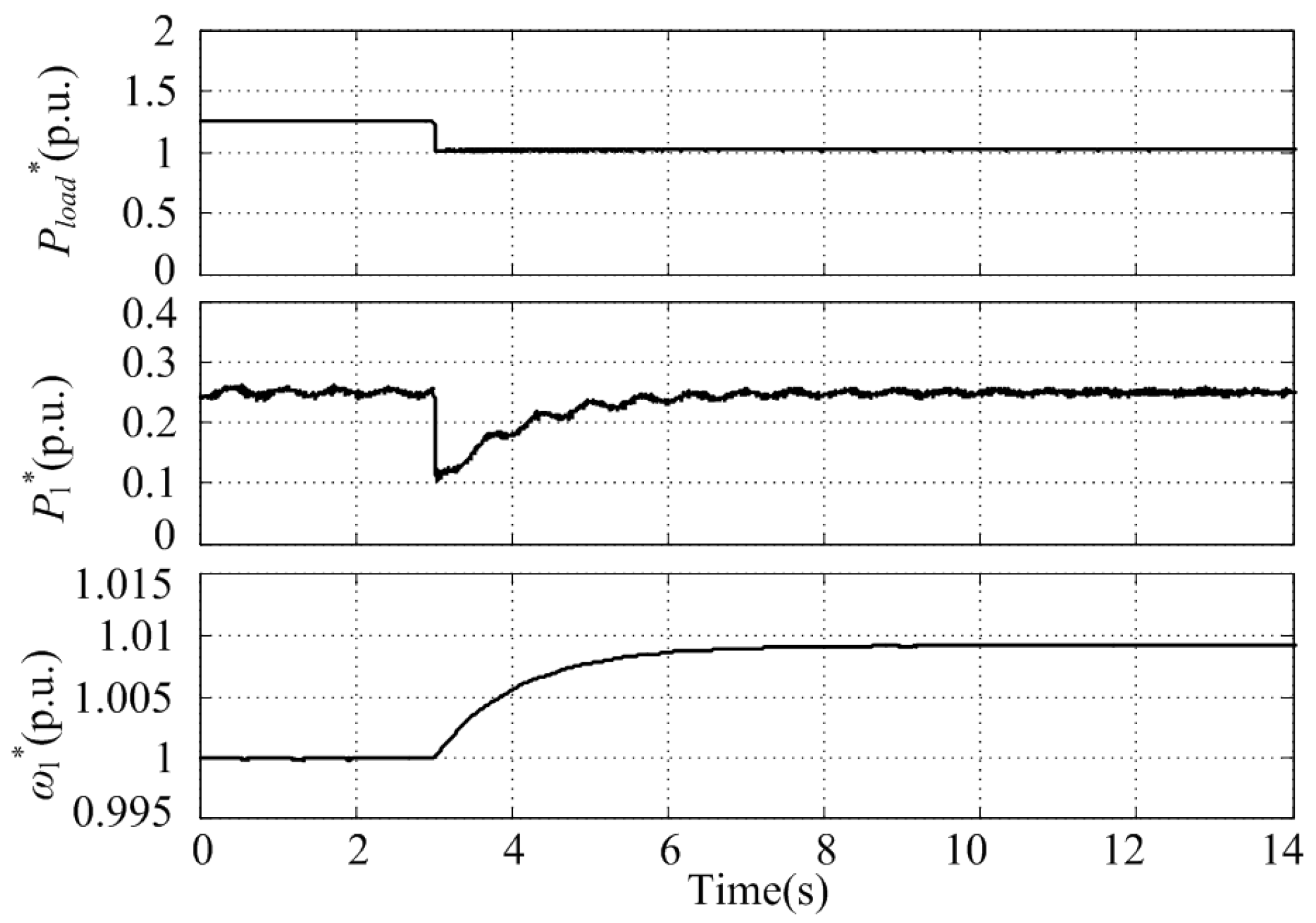
Figure 17.
Transient response for system 1 (a) ; (b) .

Figure 18.
Transient response for system 2 (a) ; (b) .

Figure 19.
Stability of system 1 under different values of H1 (a) Output active power deviation and (b) Frequency deviation when H1 = 0.06; (c) Output active power deviation and (d) Frequency deviation when H1 = 3; (e) Output active power deviation and (f) Frequency deviation when H1 = 9.
Figure 19.
Stability of system 1 under different values of H1 (a) Output active power deviation and (b) Frequency deviation when H1 = 0.06; (c) Output active power deviation and (d) Frequency deviation when H1 = 3; (e) Output active power deviation and (f) Frequency deviation when H1 = 9.

Figure 20.
Stability of system 2 under different values of H1 (a) Output active power deviation and (b) Frequency deviation when H1 = 0.06; (c) Output active power deviation and (d) Frequency deviation when H1 = 3; (e) Output active power deviation and (f) Frequency deviation when H1 = 9.
Figure 20.
Stability of system 2 under different values of H1 (a) Output active power deviation and (b) Frequency deviation when H1 = 0.06; (c) Output active power deviation and (d) Frequency deviation when H1 = 3; (e) Output active power deviation and (f) Frequency deviation when H1 = 9.

Table 1.
Parameters of system 1.
| Parameter | Value | Parameter | Value |
|---|---|---|---|
| capacity reference, Sb | 10 kVA | Voltage reference, Ub | 0.3102 kV |
| SVSG | 0.25 (p.u.) | SSG | 1 (p.u.) |
| Udc_VSG | 0.8 kV | USG(L_L) | 0.38 kV |
| HSG | 5 s | DSG | 2 (p.u.) |
| Droop coefficient of P-V, KVSG | 0.1 | VSGvirtual impedance, Xx | 0.2 (p.u.) |
| Line resistancein VSG side, R1 | 0.0042 (p.u.) | Line resistancein SG side, R2 | 0.0062 (p.u.) |
| Line reactancein VSG side, X1 | 0.01327 (p.u.) | Line reactancein SG side, X2 | 0.0198 (p.u.) |
| SG direct-axis armature reactance, Xd | 0.3 (p.u.) | SG quadrature-axis armature reactance, Xq | 0.3 (p.u.) |
| SGdroop control coefficient, Kd1 | 25 | ωref | 314 rad/s |
| Pref_VSG | 0.25 (p.u.) | Pref_SG | 1 (p.u.) |
| Qref_VSG | 0 | Qref_SG | 0 |
| Filter resistor, Rf | 0.037 Ω | Filter inductance, Lf | 3.1 mH |
| Filter capacitor, Cf | 8.17 μF |
Table 2.
Parameters of system 2.
| Parameter | Value | Parameter | Value |
|---|---|---|---|
| Capacity reference, Sb | 10 kVA | Voltage reference, Ub | 0.3102 kV |
| SVSG1 | 1 (p.u.) | SVSG2 | 1 (p.u.) |
| Udc_VSG1 | 0.8 kV | Udc_VSG2 | 0.8 kV |
| HVSG2 | 5 s | DVSG2 | 2 |
| VSG1 droop coefficient of P-V, KVSG1 | 0.1 | VSG2 droop coefficient of P-V, KVSG2 | 0.1 |
| VSG1 virtual impedance, Xx1 | 0.2 (p.u.) | VSG2 virtual impedance, Xx2 | 0.3 (p.u.) |
| Line resistance in VSG1 side, R1 | 0.0062 (p.u.) | Line resistance in VSG2 side, R2 | 0.0062 (p.u.) |
| Line reactance in VSG1 side, X1 | 0.0198 (p.u.) | Line reactance in VSG2 side, X2 | 0.0198 (p.u.) |
| VSG2 droop control coefficient, Kd2 | 25 | ωref | 314 rad/s |
| Pref_VSG1 | 0.25 (p.u.) | Pref_VSG2 | 1 (p.u.) |
| Qref_VSG1 | 0 | Qref_VSG2 | 0 |
| Filter resistor of VSG1, Rf1 | 0.037 Ω | Filter inductance of VSG1, Lf1 | 3.1 mH |
| Filter capacitor of VSG1, Cf1 | 8.17 μF | Filter resistor of VSG2, Rf2 | 0.037 Ω |
| Filter inductance of VSG2, Lf2 | 3.1 mH | Filter capacitor of VSG2, Cf2 | 8.17 μF |
© 2018 by the authors. Licensee MDPI, Basel, Switzerland. This article is an open access article distributed under the terms and conditions of the Creative Commons Attribution (CC BY) license (http://creativecommons.org/licenses/by/4.0/).
Share and Cite
MDPI and ACS Style
Yuan, C.; Xie, P.; Yang, D.; Xiao, X. Transient Stability Analysis of Islanded AC Microgrids with a Significant Share of Virtual Synchronous Generators. Energies 2018, 11, 44. https://doi.org/10.3390/en11010044
AMA Style
Yuan C, Xie P, Yang D, Xiao X. Transient Stability Analysis of Islanded AC Microgrids with a Significant Share of Virtual Synchronous Generators. Energies. 2018; 11(1):44. https://doi.org/10.3390/en11010044
Chicago/Turabian StyleYuan, Chang, Peilin Xie, Dan Yang, and Xiangning Xiao. 2018. "Transient Stability Analysis of Islanded AC Microgrids with a Significant Share of Virtual Synchronous Generators" Energies 11, no. 1: 44. https://doi.org/10.3390/en11010044
Note that from the first issue of 2016, this journal uses article numbers instead of page numbers. See further details here.