A Comparison of Thermal Models for Temperature Profiles in Gas-Lift Wells

1
Chinese Academy of Geological Sciences, No. 26 Baiwanzhuang Street, Beijing 100037, China
2
Petroleum Systems Engineering, University of Regina, Regina, SK S4S 0A2, Canada
3
Daqing Oilfield Exploration and Development Institute, Daqing 163712, China
*
Author to whom correspondence should be addressed.
Energies 2018, 11(3), 489; https://doi.org/10.3390/en11030489
Submission received: 26 January 2018
/
Revised: 17 February 2018
/
Accepted: 22 February 2018
/
Published: 26 February 2018
Abstract
:Gas lift is a simple, reliable artificial lift method which is frequently used in offshore oil field developments. In order to enhance the efficiency of production by gas lift, it is vital to exactly predict the distribution of temperature-field for fluid within the wellbore. A new mechanistic model is developed for computing flowing fluid temperature profiles in both conduits simultaneously for a continuous-flow gas-lift operation. This model assumes steady heat transfer in the formation, as well as steady heat transfer in the conduits. A micro-units discrete from the wellbore, whose heat transfer process is analyzed and whose heat transfer equation is set up according to the law of conservation of energy. A simplified algebraic solution to our model is conducted to analyze the temperature profile. Sensitivity analysis was conducted with the new model. The results indicate that mass flow rate of oil and the tubing overall heat transfer coefficient are the main factors that influence the temperature distribution inside the tubing and that the mass flow rate of oil is the main factor affecting temperature distribution in the annulus. Finally, the new model was tested in three various wells and compared with other models. The results showed that the new model is more accurate and provides significant references for temperature prediction in gas lift well.
1. Introduction
As reservoir pressure declines, the production decreases and there is a need to use artificial lift methods to increase the production rate [1,2,3]. Gas lift is one of the industry’s choices to develop low pressure fields. The gas, after being injected into the casing-tubing annulus at the wellhead, enters the production tubing via a gas lift valve situated in the gas lift mandrel [4,5]. Then the gas mixes with the produced fluids in the tubing, aerating the produced fluids and causing them to rise to the surface [6]. Gas-lift technology has evolved and matured over the years since the pioneering works of Poettmann-Carpenter [7] and Bertuzzi et al. [8] in the early 1950s. Through years of development, gas-lift technique has matured gradually.
Fluid temperature enters into a variety of petroleum production operations calculations, including well drilling and completions, production facility design, controlling solid deposition, and analyzing pressure transient test data [9]. In terms of gas-lift design, the thermally actuated safety valves have been used since the 1930s in many different applications. A thermally actuated safety valve would rely on a change in temperature between normal operation and an undesirable flow event [10]. In order to realize the productivity calculation during gas-lift and explore the oil-gas resource efficiently, it is vital to exactly predict distribution of temperature-field for fluid within the wellbore.
Many scholars have carried out different studies on rock heat-transfer within gas strata of wellbores over the last few decades. One of the earliest works on predicting temperature profiles in a flowing well was presented by Kirkpatrick [11] in the early 1950s. He presented a simple flowing-temperature-gradient chart that could be used to predict gas-lift valve temperatures at the injection depth. Ramey and Edwardson [12] presented a theoretical model to estimate fluid temperature as a function of well depth and production time. The model has been widely used in both geothermal and petroleum industries. However, the effects of kinetic energy and friction were ignored in the model, and therefore the model is only applicable to single-phase flow. There have been many modified temperature models (Shiu and Beggs [13]; Hasan et al. [14,15]) for two-phases flow in wellbore. Sagar et al. [16] extended Ramey’s model to multiphase flow in wellbore by considering kinetic energy and Joule-Thompson expansion effects. Tartakovsky [17] present a Lagrangian particle model for multiphase multicomponent fluid flow, based on smoothed particle hydrodynamics. Farrokhpanah [18] further developed this method to study the heat transfer and phase change which was existed during CO2 migrating upwards along vertical leakage paths in wellbore [19]. Alves [20] presents a general and unified equation for flowing temperature prediction that is applicable for the entire range of inclination angles. The equation degenerates into Ramey’s equations for ideal gas or incompressible liquid and into the Coulter and Bardon equation, with the appropriate assumptions. In addition, many scholars (Yanmin et al. [21]; Lindeberg [22]; Hamedi [23]; Kabir et al. [24]) further extended its application on the basis of previous studies. In 2013, Duan [25] predicted the temperature profile in a waxy oil-gas pipe flow and he considered the different parameters and used the heat balance in his model. Cheng [26] represented a model for distribution of thermal properties and oil saturations in steam injection wells. He involved the temperature logs in his studies. Han [27] studied the transient two phase fluid and heat transfer model with periodical electric heating. He analyzed the heat-flux conservation among different layers and presented the derivatives of temperature in location and time. The solution was obtained numerically to capture the temperature/pressure distribution profiles under transient conditions.
To design a gas-lift system from the viewpoints of both fluid flow and valve mechanics, an accurate knowledge of fluid temperature in both strings is very desirable. This paper presents a new model to describe the temperature distribution in annulus and tubing during the operation of gas lift. We also discuss the influence of relevant parameters. Moreover, this methodology is applied to some field cases to compare with other models.
2. Methodology
Temperature distribution in the wellbore is very important during the gas lift operation, which laid the foundations for the analysis and prediction of fluid flow in oil pipe, and the determination of position of the suction valve, etc. Numerical simulation calculation with all factors was difficult to achieve for the complex steam injection process in the wellbore.
Figure 1 depicts a small element of a borehole section with a tubing string at center. As shown, gas will be injected into the annulus and mixed with the fluid from the reservoir, and then flow to the surface through the tubing. There will be two heat transfers in this process, which are the one between fluid in the annulus and the formation and the one between fluid inside tubing and fluid in the annulus. Therefore, the following assumptions are made in model formulation.
2.1. Assumptions
- (1)
- The thermal conductivity of casing is assumed to be infinity.
- (2)
- The geothermal gradient behind the annulus is not affected by borehole fluid.
- (3)
- Heat capacity of the fluid is constant.
- (4)
- Friction-induced heat is negligible.
2.2. Governing Equation
(1) Flow in the annulus
Consider the heat transfer in the annulus of length L during a short time period of Δt. Heat energy balance is given by:
where Qa,in is the heat energy brought into the annular element by the annular fluid due to convection; qf is the heat transfer from the formation rock to the annulus due to conduction; qt is the heat transfer from the tubing fluid to the annulus due to conduction; Qa,out is the heat energy carried away from the annular element by the annular fluid due to convection; Qa,change is the change of heat energy in the annular fluid in the element.
Substitute equations of above coefficients into Equation (1) and the governing equation for annulus temperature Ta can be obtained (Appendix A):
where
(2) Flow in the tubing
Consider the heat transfer in the tubing element of length ΔL during a time period of Δt. Heat balance is given by
where Qt,in is the heat energy brought into the tubing element by the tubing fluid due to convection; qt is the heat transfer from the tubing fluid to the annulus due to conduction; Qt,out is the heat energy carried away from the tubing element by the tubing fluid due to convection; Qt,change is the change of heat energy in the tubing fluid in the element.
Substituting the coefficient equations into Equation (6) the governing equation for tubing temperature Tt can be obtained (Appendix A):
where
2.3. Boundary Conditions
The boundary condition for solving Equation (2) is expressed as:
The boundary condition for solving Equation (7) is expressed as:
where
where TJT is the gas temperature drop due to the Joule–Thomason cooling effect [28] which is assumed to be 0.16Ta gas under sonic flow conditions across the gas injection valve, Equation (10) is expressed as:
2.4. Analytical Solution
The details of solving the Equations (2) and (7) are presented in Appendix A. The resultant solutions are summarized as follows:
3. Results and Discussion
3.1. Sensitivity Analysis
There are plenty of factors that affect the temperature distribution of fluid within tubing and casing, and production tools and the production system change the nature of each factor. Moreover, there is no correlation with each other. Therefore, this paper makes a comparison on the basis of the first law of thermodynamics and reduced temperature for convenient sensitivity analysis and for creating formulas. A base value is set and the single factor is fluctuated above and below that basic value. Afterwards, the range for the temperature within the tubing, casing and the entire wellbore is calculated (according to basic value). In this way, the calculation results are comparable.
3.1.1. Sensitivity Analysis Method
After variation amplitude value is computed based on the aforementioned approach, the influence degree of each factor is then calculated according to Equation (14):
where ki is the extent of influence and ai is the gradient of absolute value. The result shows which factor has the biggest impact on temperature within the wellbore under the same fluctuation range.
3.1.2. Basic Parameters
In order to determine the parameters that affect temperature distribution (namely, key controlling factors) and the extent of their influence, this paper makes parameter sensitive analysis for each production index, based on exploring internal energy of the fluid within the tubing and casing, and then confirms its controlling factors according to heat gradient (rate) with the variation of different parameters. The basis of the project of sensitivity analysis is presented in Table 1.
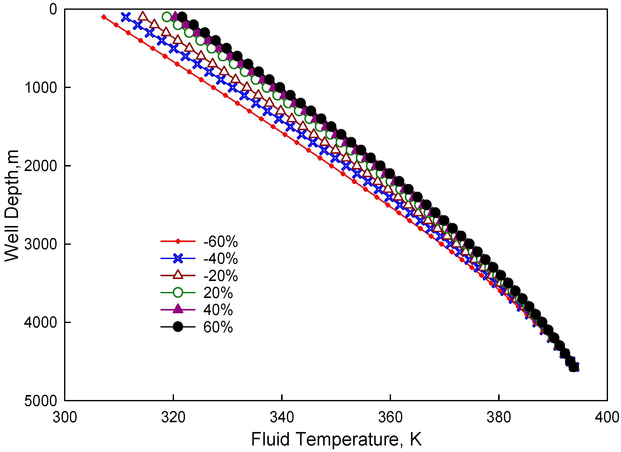
Each average value (Table 1) within the range defined by coefficient intervals is selected as the basic contrasting evidence, and Figure 2 shows the temperature profile curve in the annulus, tubing and geothermal gradient.
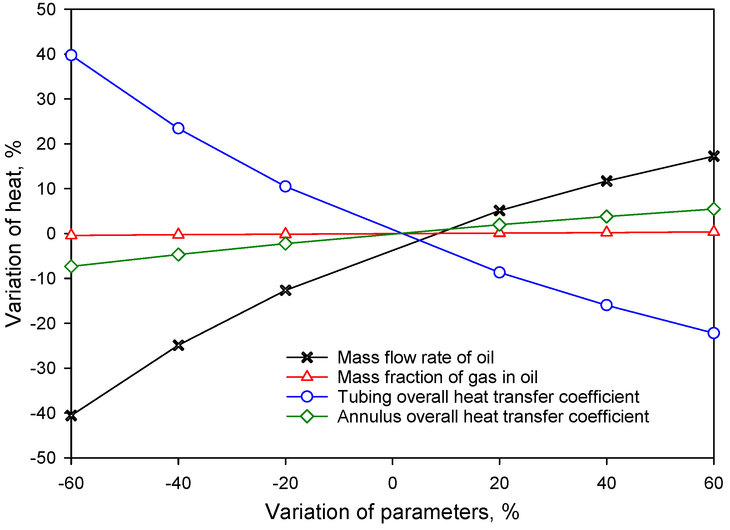
Mass flow rate of oil, mass fraction of gas in oil, tubing overall heat transfer coefficient, annulus overall heat transfer coefficient are shifted 20%, 40% and 60% up or down, respectively; then the resulting temperature change is calculated (Table 2).
3.1.3. Major Factors Affecting Temperature Distribution inside Tubing
Figure 3 shows that along with the increase of mass flow rate of oil, temperature within the tubing is rises as well. This is because more heat in the formation fluid is carried out of the oil well with the increase of mass flow rate of oil and the duration of the external heat transfer for fluid within the tubing is shortened during flow, which wholly improves the temperature within the tubing, and such an increase becomes smaller and smaller.
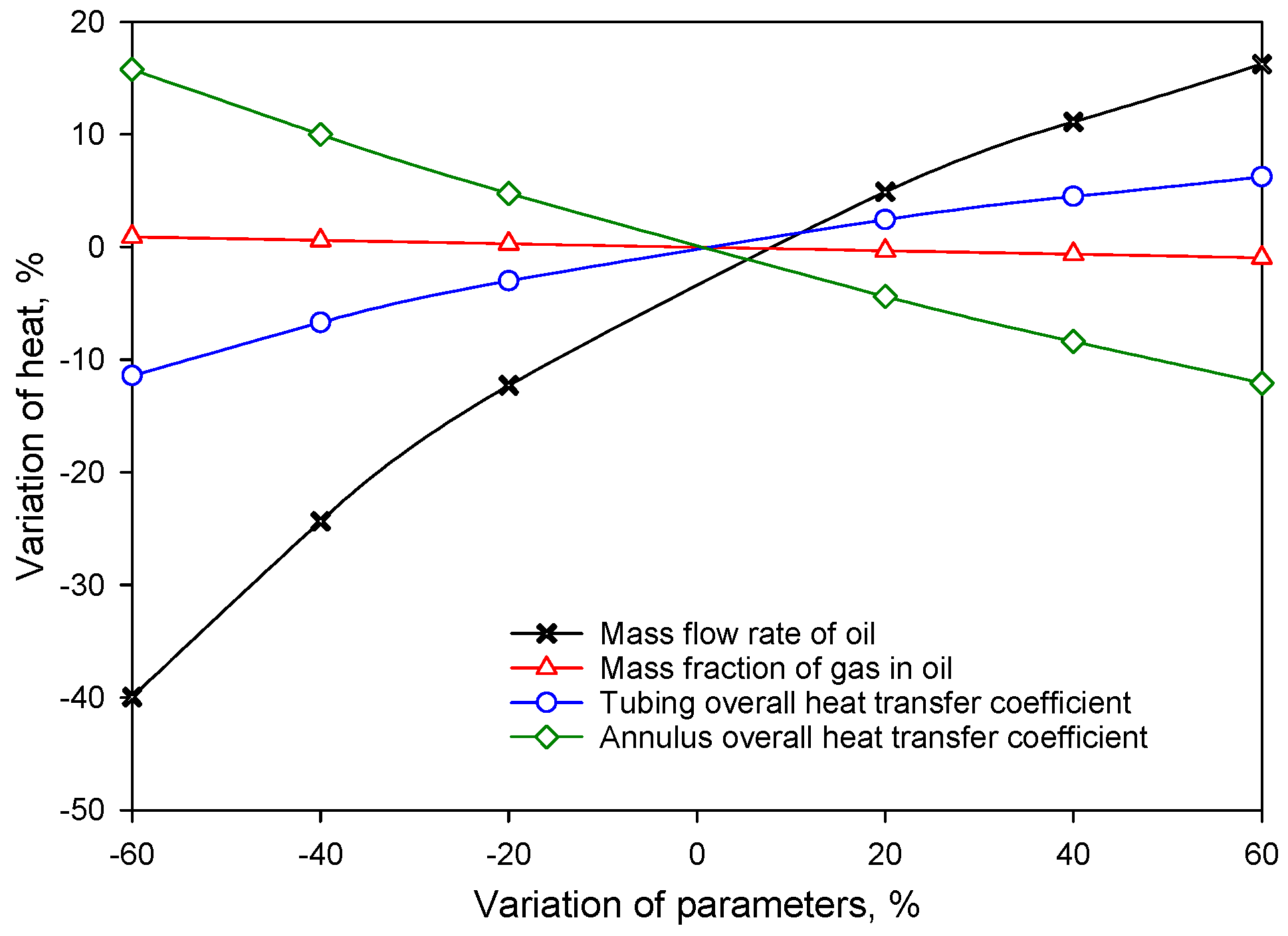
Figure 4 and Table 3 suggests that when each variable decreases, the influence of each factor on temperature within the tubing is as follows (from great to small): the mass flow rate of oil, the tubing overall heat transfer coefficient, the annulus overall heat transfer coefficient, and the mass fraction of gas in oil.
3.1.4. Major Factors Affecting Temperature Distribution in the Annulus
Figure 5 shows that along with the increase of the mass flow rate of oil, the temperature within the casing also rises. This is because that the increase in temperature within the tubing enlarges the temperature differences between the both sides of tubing wall and heat transfer is thus enhanced, which leads to the rise in fluid temperature within casing.
3.2. Case Study
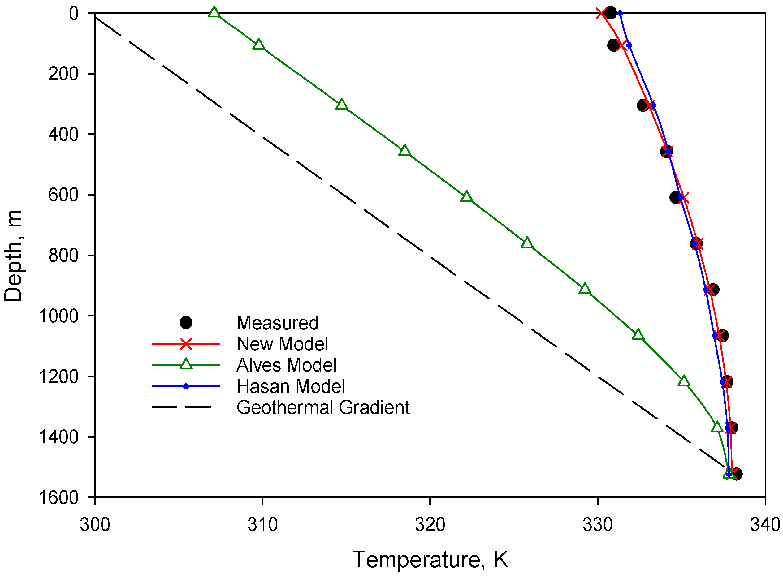
Two thermal models which developed by Hasan [14] and Alves [20] are adopted to compare with our model.
3.2.1. Case 1
This field example is given to show the application of the new model. This case is taken from the published work of Hasan [14]. Table 5 presents all of the parameters used to compute the pressure and temperature traverses.
In this well, large discontinuity in the in-situ gas volume-fraction occurs at 2500 ft where the lift gas is introduced through the annulus. The temperature profile below the injection point is computed by using a simplified model from our model. The assumptions of the simplified model are that a single phase fluid flows in the tubing and the heat transfer in annulus is neglected.
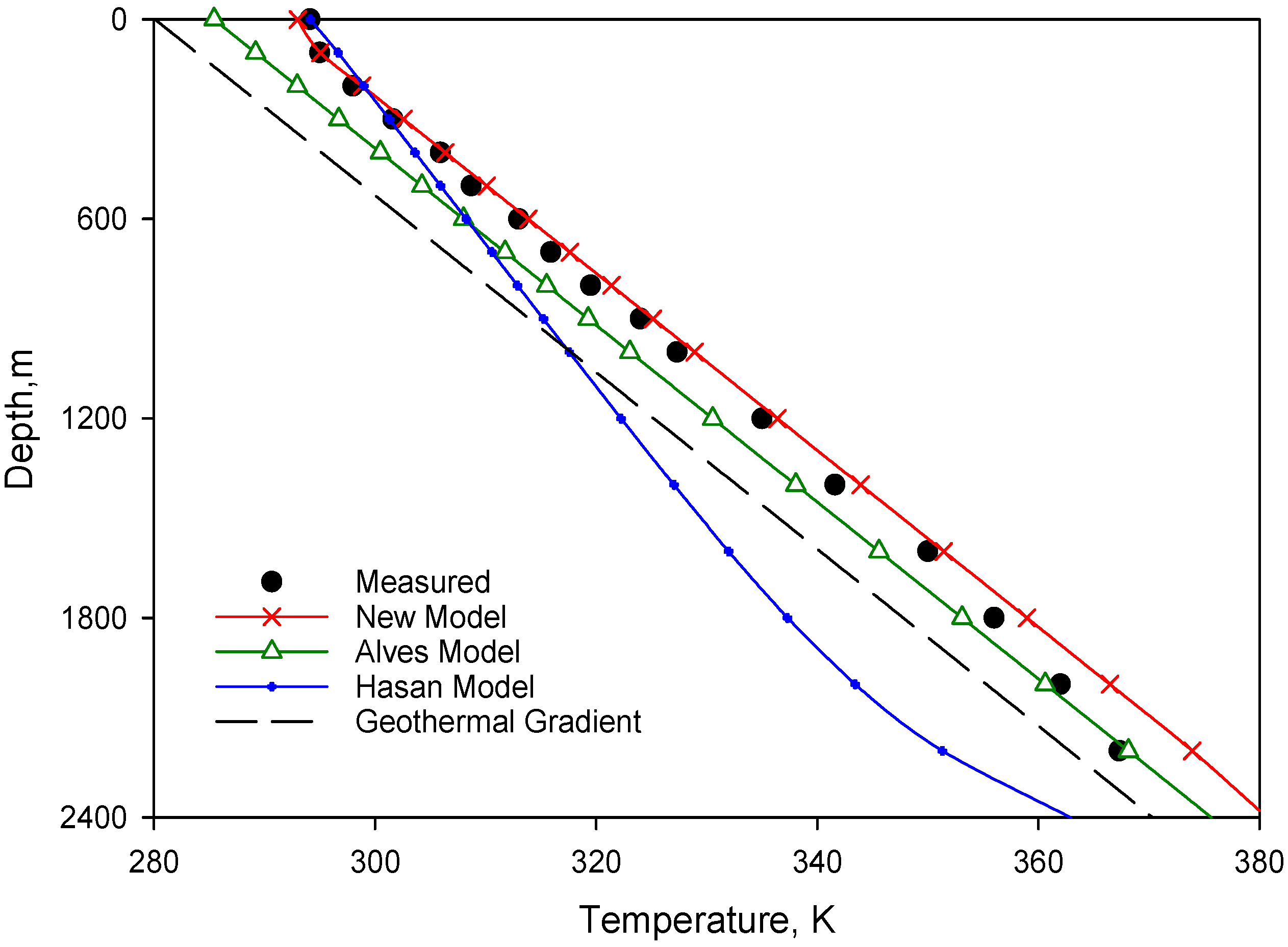
The corresponding tubing temperature profiles, both measured and computed, are shown in Figure 7. A good agreement is obtained between this model and measurement for temperature profiles.
However, the same was not true for the Alves Model. This is because that the Alves Model is derived for simulating multi-phases flowing in tubing and do not consider the effect made by heat transfer in annulus.
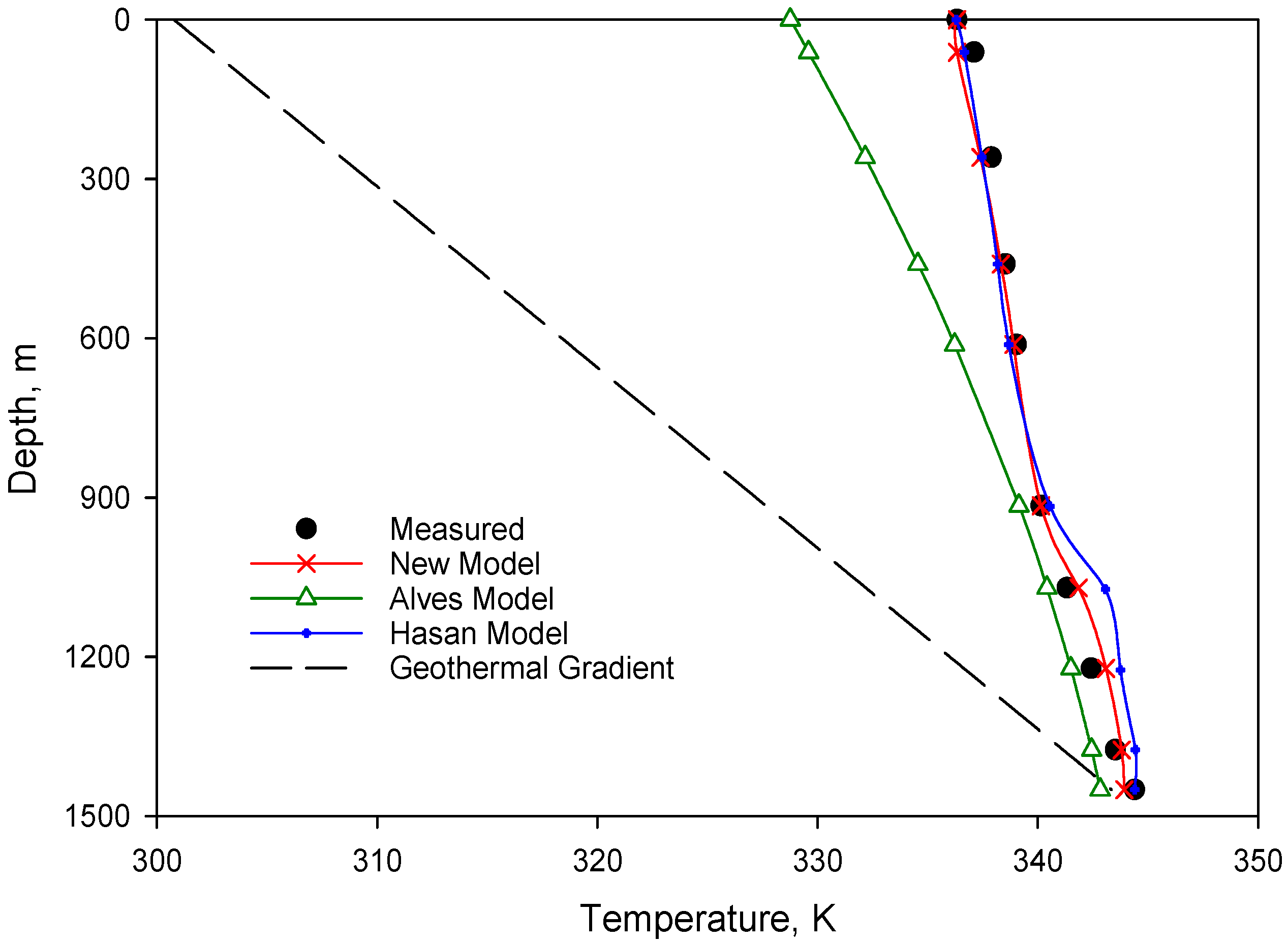
3.2.2. Case 2
The data for the O’Connor Well also comes from the published work of Hasan [14]. All the parameters used to compute the pressure and temperature profiles are presented in Table 6. Because the geothermal gradient was not reported, we obtained a match by adjusting it.
For the O’Connor Well, Figure 8 shows that a good agreement in temperature occurs at shallower depths where two phases flow is prevalent but to a lesser degree near the point of gas injection. Just as mentioned in the literature, two possible reasons exist for this mismatch [14].
Either the geothermal gradient is substantially different below the point of gas injection, or short-duration station stops did not allow for the thermometer to equilibrate with the fluid temperature. There is significant error near injection point.
3.2.3. Case 3
Luo Wei [29] computed temperature distribution of gas-lift production in a certain oil field. This oil-field was mined by adopting the gas-lift annulus, and in order to solve the problem of wax growth at 2624.67 ft above the oil well, the experiment was performed in which experiment the temperature of produced liquid within the wellbore was increased by trying to add the injection temperature. Afterwards, research analysis is conducted by taking data in this oil field as a case. Table 7 lists the basic parameters of the well and measured data.
For the Luo Wei well, Figure 9 shows that good agreement in temperature profile at shallower depths exists, but to a lesser degree around the point of gas injection. The measured temperature profile is only from the surface to the injection point.
The possible reason for this mismatch is that the geothermal gradient is substantially different owing to the different formation properties below the point of gas injection and this difference may have an effect on the temperature distribution around the injection point.
4. Conclusions
The following conclusions are drawn:
- (1)
- A new mechanistic model is developed for computing flowing fluid temperature profiles in both conduits simultaneously for a continuous-flow gas-lift operation. The model assumes steady heat transfer in the formation, as well as steady heat transfer in the conduits. This work also presents a simplified algebraic solution to the analytic model, affording easy implementation in any existing program. An accurate fluid temperature computation should allow improved gas-lift design.
- (2)
- Comparisons of the Hasan model, Alves model and the new model with data from three actual well show that the temperature profile given by the new model has a better accuracy than that of other models.
- (3)
- A sensitivity analysis is conducted with the new model. The results indicate that:
- (a)
- The mass flow rate of oil and the tubing overall heat transfer coefficient are the main factors that influence the temperature distribution inside the tubing;
- (b)
- The mass flow rate of oil is the main factor affecting temperature distribution in the annulus. The annulus overall heat transfer coefficient of the annulus and overall heat transfer coefficient of the tubing are the next factors.
Author Contributions
Langfeng Mu and Qiushi Zhang conceived and designed the research contents and simulations; Qi Li analyzed the data; Langfeng Mu performed the calculation and wrote the paper; Fanhua Zeng and Qiushi Zhang checked the paper.
Conflicts of Interest
The authors declare no conflict of interest.
Nomenclature
| Ca | the heat capacity of annular fluid |
| Co | the heat capacity of the produced fluid from the oil reservoir |
| Ct | the heat capacity of the tubing fluid |
| dt | the inner diameter of the tubing |
| Dc | the outer diameter of casing |
| Dt | the outer diameter of tubing |
| Dw | the diameter of the wellbore (to sandface) |
| Kt | the thermal conductivity of tubing |
| qf | the heat transfer from the formation rock to the annulus due to conduction |
| qt | heat transfer from the tubing fluid to the annulus due to conduction |
| Qa,in | The heat energy brought into the annular element by the annular fluid due to convection |
| Qa,out | the heat energy carried away from the annular element by the annular fluid due to convection |
| Qa,change | the change of heat energy in the annular fluid in the element |
| Qt,in | the heat energy brought into the tubing element by the tubing fluid due to convection |
| Qt,out | the heat energy carried away from the tubing element by the tubing fluid due to convection |
| Qt,change | the change of heat energy in the tubing fluid in the element |
| r | the radial distant |
| Ta0 | surface temperature, k |
| Ta,L | the temperature of annular fluid at location L |
| Ta,L+ΔL | the temperature of annular fluid at location L + ΔL |
| Tc | the temperature in the cement sheath in the radial direction |
| Tg | the geo-temperature at the depth L |
| TJT | the gas temperature drop due to the Joule–Thomason cooling effect |
| Tt | the temperature of the tubing fluid at the depth L |
| Tt,L+ΔL | the temperature of the tubing fluid at location L + ΔL |
| Ttb | the temperature in the tubing in the radial direction |
| ma | the mass flow rate of annular fluid |
| mo | The mass flow rate of the produced fluid from the oil reservoir |
| mt | the mass flow rate of the tubing fluid |
Appendix A
(1) Flow in the annulus
Consider the heat transfer in the annulus of length L during a short time period of Δt. Heat energy balance is given by:
The Qa,in term can be expressed as:
The qf term is formulated as:
The qt term is expressed as:
The Qa,out term is formulated as:
The Qa,change term is expressed as:
Substituting Equations (A2) through (A6) into Equation (A1) gives
which is rearranged to get:
where the temperature gradient terms can be formulated as:
and:
Substituting Equations (A9) and (A10) into Equation (A8) gives:
Dividing all the terms of this equation by ΔLΔt yields:
For infinitesimal of ΔL and Δt, this equation becomes:
Substituting for Equation (A13) and rearranging the latter yields:
where
Substituting for Equation (A14) yields the governing equation for annular temperature Ta:
(2) Flow in the tubing
Consider the heat transfer in the tubing element of length ΔL during a time period of Δt. Heat balance is given by
The Qt,in term can be expressed as
The Qt,out term is formulated as
The Qt,change term is expressed as
Substituting Equation (A4) and Equation (A20) through (A22) for Equation (A19) gives
which is rearranged to yield:
where the temperature gradient terms can be formulated as:
Substituting Equation (A25) for Equation (A24) gives:
Dividing all the terms of this equation by ΔLΔt yields:
For infinitesimal ΔL and Δt, this equation becomes:
Substituting for Equation (A28) and rearranging the later gives the governing equation for tubing temperature Tt:
where
Boundary conditions:
The boundary condition for solving Equation (A18) is expressed as:
The boundary condition for solving Equation (A29) is expressed as:
where
Under sonic flow conditions, Equation (A32) is expressed as:
(3) Analytical Solution
Equation (A18):
Equal to:
Equation (A29):
Equal to:
Solutions to these equations are given in Appendix A. The resultant solutions are summarized as follows.
The temperature in the annulus is expressed as follows:
The temperature inside the tubing is expressed as follows:
C1, C2 which in the Equations (A36) and (A37) are undetermined coefficients (calculated by boundary conditions), where:
and then apply the boundary conditions:
According to (A36), this yields can get the following:
Apply the boundary condition:
According to (A37), this yields can get the following:
where Tmax is:
The Equation (A45) can be shown as follows:
The Equation (A46) can be shown as:
where
Using simultaneous Equations (A48) and (A49), this yields can get the following:
Finally, substituting C1, C2 for Equations (A36) and (A37), where the analytical solution is shown as follows:
References
- Clegg, J.D.; Bucaram, S.M.; Hein, N.W., Jr. Recommendation and Comparisons for Selecting Artificial-Lift Methods. J. Pet. Technol. 1993, 45. [Google Scholar] [CrossRef]
- Fleyfel, F.; Meng, W.; Hernandez, O. Production of Waxy Low Temperature Wells with Hot Gas Lift. In Proceedings of the SPE Annual Technical Conference and Exhibition, Houston, TX, USA, 26–29 September 2004; pp. 26–29. [Google Scholar] [CrossRef]
- Aliyeva, F.; Novruzaliyev, B. Gas Lift—Fast and Furious. In Proceedings of the SPE Annual Caspian Technical Conference & Exhibition, Baku, Azerbaijan, 4–6 November 2015; pp. 4–6. [Google Scholar] [CrossRef]
- Guo, B.; Duan, S.; Ghalambor, A. A Simple Model for Predicting Heat Loss and Temperature Profiles in Insulated Pipelines. Soc. Pet. Eng. 2006, 21. [Google Scholar] [CrossRef]
- Muradov, K.M.; Davies, D.R. Novel Analytical Methods of Temperature Interpretation in Horizontal Wells. Soc. Pet. Eng. 2011, 16, 637–647. [Google Scholar] [CrossRef]
- Brown, K.E. The Technology of Artificial Lift Methods; U.S. Department of Energy, Office of Scientific and Technical Information: Oak Ridge, TN, USA, 1984; Volume 4. [Google Scholar]
- Poettmann, F.H.; Carpenter, P.G. The Multiphase Flow of Gas, Oil, and Water through Vertical Flow Strings with Application to the Design of Gas-Lift Installations; American Petroleum Institute: New York, NY, USA, 1952. [Google Scholar]
- Bertuzzi, A.F.; Welchon, J.K.; Poettmann, F.H. Description and Analysis of an Efficient Continuous-Flow Gas-Lift Installation. J. Pet. Technol. 1953, 5, 271–278. [Google Scholar] [CrossRef]
- Hasan, A.R.; Kabir, C.S. Wellbore Heat-Transfer Modeling and Applications. J. Pet. Sci. Eng. 2012, 86, 127–136. [Google Scholar] [CrossRef]
- Gilbertson, E.; Hover, F.; Freeman, B. A Thermally Actuated Gas-lift Safety Valve. SPE Prod. Oper. 2013, 28, 77–84. [Google Scholar] [CrossRef]
- Kirkpatric, C.V. Advanced in Gas Lift Technology; American Petroleum Institute: New York, NY, USA, 1959. [Google Scholar]
- Ramey, H.J., Jr. Wellbore Heat Transmission. J. Pet. Technol. 1962, 14, 427–435. [Google Scholar] [CrossRef]
- Shiu, K.C.; Beggs, H.D. Predicting Temperatures in Flowing Oil Wells. J. Energy Res. Technol. 1980, 102, 2–11. [Google Scholar] [CrossRef]
- Hasan, A.R. A Mechanistic Model for Computing Fluid Temperature Profiles in Gas-Lift Wells. Soc. Pet. Eng. 1996, 11, 179–185. [Google Scholar] [CrossRef]
- Hasan, A.R.; Kabir, C.S.; Lin, D. Analytic Wellbore Temperature Model for Transient Gas-Well Testing. Soc. Pet. Eng. 2005, 8. [Google Scholar] [CrossRef]
- Sagar, R.K.; Doty, D.R.; Schmidt, Z. Predicting Temperature Pro-files in a Flowing Well. SPE Prod. Eng. 1991, 6, 441–448. [Google Scholar] [CrossRef]
- Tartakovsky, A.M.; Ferris, K.F.; Meakin, P. Lagrangian Particle Model for Multiphase Flows. Comput. Phys. Commun. 2009, 180, 1874–1881. [Google Scholar] [CrossRef]
- Farrokhpanah, A.; Bussmann, M.; Mostaghimi, J. New Smoothed Particle Hydrodynamics (SPH) Formulation for Modeling Heat Conduction with Solidification and Melting. Numer. Heat Transf. Part B Fundam. 2017, 71, 299–312. [Google Scholar] [CrossRef]
- Zeng, F.; Zhao, G.; Zhu, L. Detecting CO2 leakage in Vertical Wellbore through Temperature Logging. Fuel 2012, 94, 374–385. [Google Scholar] [CrossRef]
- Alves, I.N.; Alhanati, F.J.S.; Shoham, O. A Unified Model for Predicting Flowing Temperature Distribution in Wellbores and Pipelines. Soc. Pet. Eng. 1992, 7, 363–367. [Google Scholar] [CrossRef]
- Yu, Y.; Lin, T.; Xie, H.; Guan, Y.; Li, K. Prediction of Wellbore Temperature Profiles During Heavy Oil Production Assisted with Light Oil Lift. Soc. Pet. Eng. 2009. [Google Scholar] [CrossRef]
- Lindeberg, E. Modelling Pressure and Temperature Profile in a CO2 Injection well. Energy Procedia 2011, 4, 3935–3941. [Google Scholar] [CrossRef]
- Hamedi, H.; Rashidi, F.; Khamehchi, E. Numerical Prediction of Temperature Profile During Gas Lifting. Pet. Sci. Technol. 2011, 29, 1305–1316. [Google Scholar] [CrossRef]
- Kabir, C.S.; Izgec, B.; Hasan, A.R.; Wang, X. Computing Flow Profiles and Total Flow Rate with Temperature Surveys in Gas Wells. J. Nat. Gas Sci. Eng. 2012, 4, 1–7. [Google Scholar] [CrossRef]
- Duan, J.; Wang, W.; Deng, D.; Zhang, Y.; Liu, H.; Gong, J. Predicting Temperature Distribution in the Waxy Oil-Gas Pipe Flow. J. Pet. Sci. Eng. 2013, 101, 28–34. [Google Scholar] [CrossRef]
- Cheng, W.L.; Nian, Y.L.; Li, T.T.; Wang, C.L. A Novel Method for Predicting Spatial Distribution of Thermal Properties and Oil Saturation of Steam Injection Well from Temperature Logs. Energy 2014, 66, 898–906. [Google Scholar] [CrossRef]
- Han, G.; Zhang, H.; Ling, K.; Wu, D.; Zhang, Z. A Transient Two-Phase Fluid- and Heat-Flow Model for Gas-Lift-Assisted Waxy-Crude Wells with Periodical Electric Heating. Soc. Pet. Eng. 2014, 53. [Google Scholar] [CrossRef]
- Hasan, A.R.; Kabir, C.S.; Wang, X. A Robust Steady-State Model for Flowing-Fluid Temperature in Complex Wells. Soc. Pet. Eng. 2009, 24, 269–276. [Google Scholar] [CrossRef]
- Wei, L.; Qian, Y. New Prediction Model for Temperature Distribution in Gas Lift Annulus Hot Gas Injection Wellbore. Oil Gas Field Dev. 2014, 32, 41–44. [Google Scholar]
Figure 1.
Sketch illustrating heat transfer in a wellbore section.
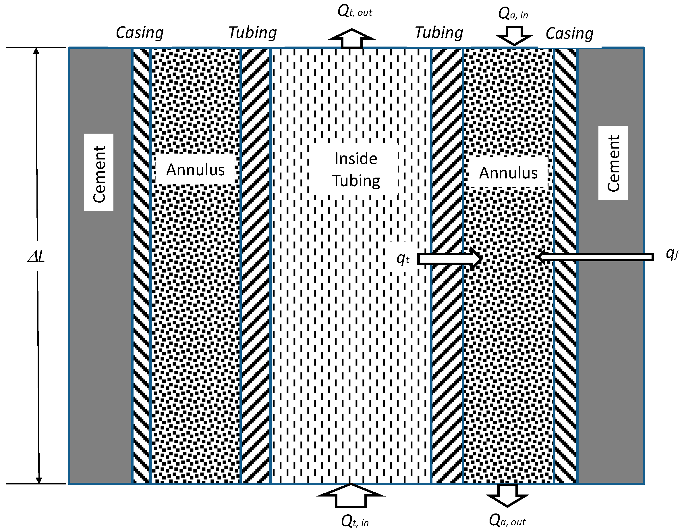
Figure 2.
Baseline for sensitivity analysis.
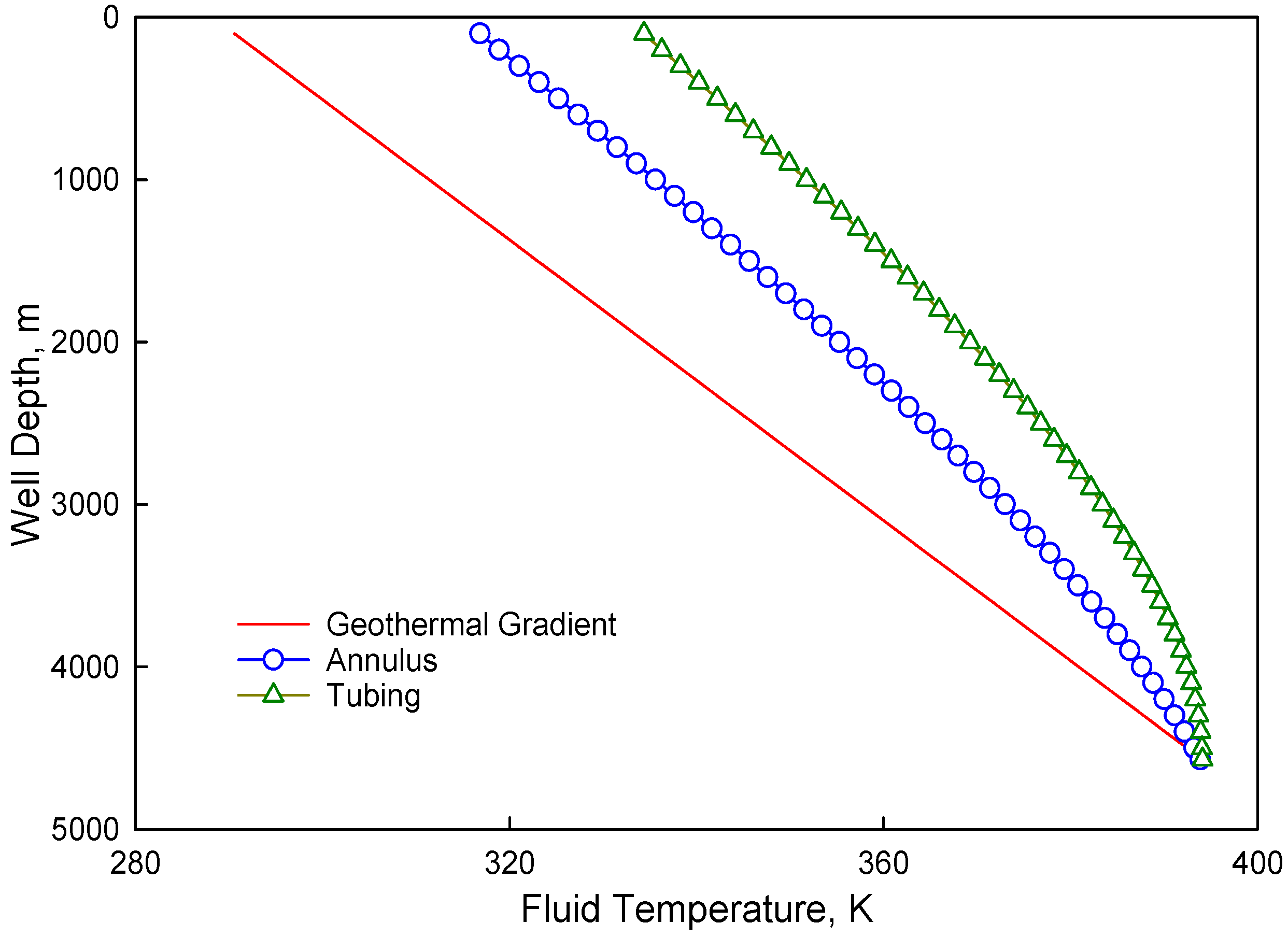
Figure 3.
Effect of oil flow rate on the temperature distribution curve in the tubing.
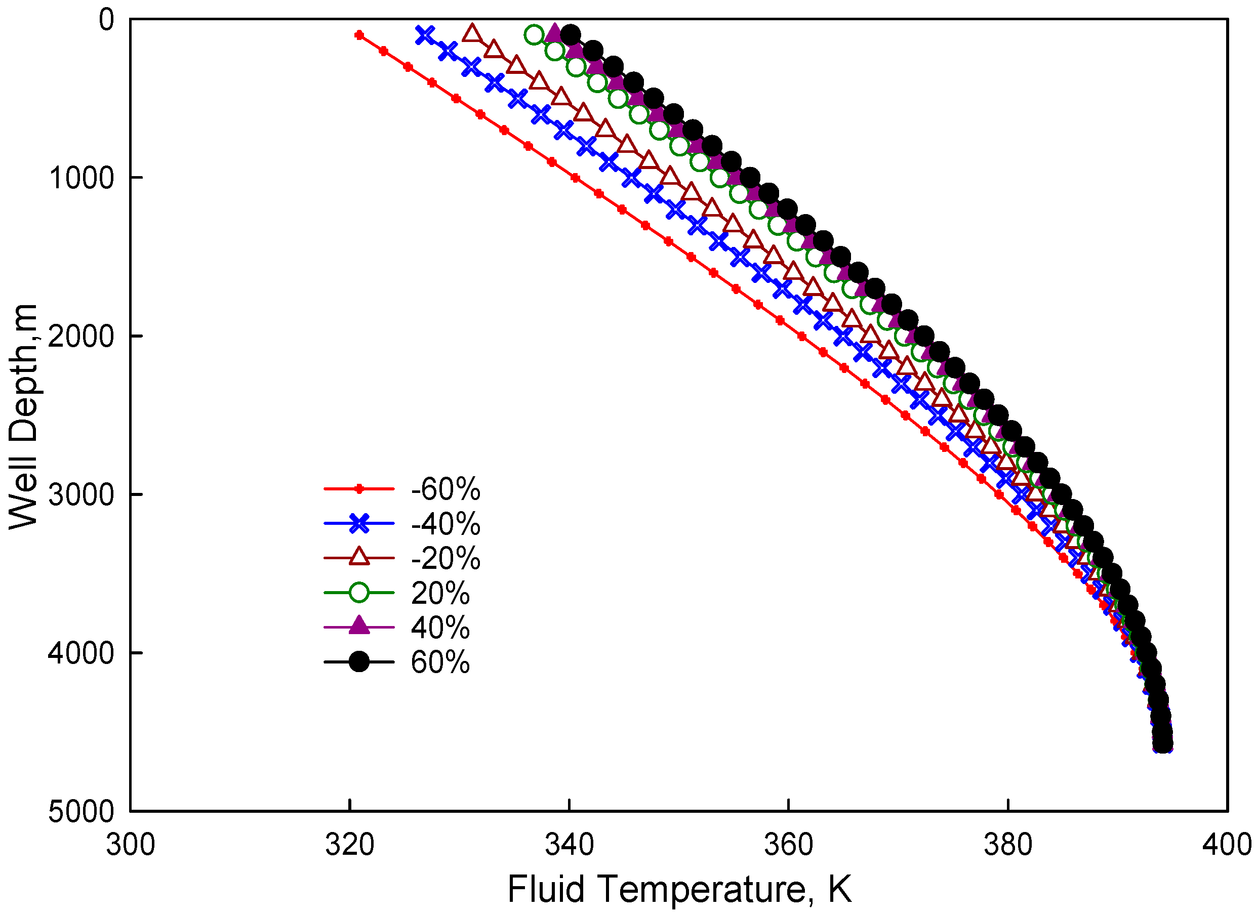
Figure 4.
Sensitive analysis for temperature variation inside tubing.

Figure 5.
Effect of oil flow rate on the temperature distribution curve in the annulus.

Figure 6.
Sensitive analysis for temperature variation in the annulus.

Figure 7.
Comparison of data for the Thompson Well.

Figure 8.
Comparison of data for the O’Connor Well.

Figure 9.
Comparison of data for the Luo Wei Well.


Table 1.
Range of Sensitive Parameter Values.
| Coefficient | Value | ||
|---|---|---|---|
| (low) | (High) | (Average) | |
| Well depth, m | ------ | ------ | 4572 |
| Casing radius, m | ------ | ------ | 0.11 |
| Tubing radius, m | ------ | ------ | 0.07 |
| Mass flow rate of oil, kg/s | 0.74 | 15.88 | 8.31 |
| Mass fraction of gas in oil | 0.05 | 0.10 | 0.075 |
| Specific heat of oil, J/(kg·K) | ------ | ------ | 1674.72 |
| Specific heat of gas, J/(kg·K) | ------ | ------ | 1046.7 |
| Tubing overall heat transfer coefficient, W/(m2·K) | 28.39 | 113.57 | 70.98 |
| Annulus overall heat transfer coefficient, W/(m2·K) | 11.36 | 22.71 | 17.03 |
| Geothermal gradient, K/m | ------ | ------ | 0.0427 |
| Bottomhole earth temperature, K | ------ | ------ | 394.26 |
| Surface earth temperature, K | ------ | ------ | 288.43 |
| Surface gas inlet temperature, K | ------ | ------ | 318.15 |
Table 2.
Values of Sensitized Parameters.
| Variation of Parameters | Mass Flow Rate of Oil | Mass Fraction of Gas in Oil | Tubing Overall Heat Transfer Coefficient | Annulus Overall Heat Transfer Coefficient |
|---|---|---|---|---|
| −60% | 3.76 | 0.060 | 45.43 | 13.63 |
| −40% | 5.28 | 0.065 | 53.94 | 14.76 |
| −20% | 6.79 | 0.070 | 62.46 | 15.90 |
| 20% | 9.82 | 0.080 | 79.49 | 18.17 |
| 40% | 11.33 | 0.085 | 88.02 | 19.31 |
| 60% | 12.85 | 0.090 | 96.53 | 20.44 |
Table 3.
Influence of factors on temperature within the tubing.
| Parameter Variations | Mass Flow Rate of Oil | Mass Fraction of Gas in Oil | Tubing Overall Heat Transfer Coefficient | Annulus Overall Heat Transfer Coefficient |
|---|---|---|---|---|
| −60% | 46.06% | 0.43% | 45.17% | 8.34% |
| −40% | 46.79% | 0.48% | 44.03% | 8.71% |
| −20% | 49.62% | 0.50% | 41.24% | 8.64% |
| 20% | 32.21% | 0.80% | 54.47% | 12.52% |
| 40% | 36.89% | 0.80% | 50.30% | 12.01% |
| 60% | 38.07% | 0.85% | 48.99% | 12.09% |
Table 4.
Influence of Factors on Temperature in the Annulus.
| Parameter Variations | Mass Flow Rate of Oil | Mass Fraction of Gas in Oil | Tubing Overall Heat Transfer Coefficient | Annulus Overall Heat Transfer Coefficient |
|---|---|---|---|---|
| −60% | 58.70% | 1.36% | 16.77% | 23.18% |
| −40% | 58.46% | 1.48% | 16.05% | 24.01% |
| −20% | 60.33% | 1.52% | 14.68% | 23.47% |
| 20% | 40.80% | 2.57% | 20.37% | 36.27% |
| 40% | 45.19% | 2.51% | 18.29% | 34.01% |
| 60% | 45.80% | 2.61% | 17.58% | 34.01% |
Table 5.
Data for the Thompson Well.
| Coefficient | Value |
|---|---|
| Total well depth, m | 1529.79 |
| Depth of gas infection, m | 731.52 |
| Casing ID, m | 0.18 |
| Tubing OD, m | 0.073 |
| Oil + water flow rate, m3/s | 0.0038 |
| Mass fraction of gas in the tubing | 0.0681 |
| Gas/liquid ratio, m3/m3 | 97.9 |
| Oil + water API gravity | 10.3 |
| Gas gravity (air = 1) | 0.61 |
| Specific heat of liquid, J/(kg·K) | 4186.8 |
| Specific heat of gas, J/(kg·K) | 1046.7 |
| Tubing overall heat transfer coefficient, W/(m2·K) | 56.78 (Hasan and Alves), 39.75 (New model) |
| Annulus overall heat transfer coefficient, W/(m2·K) | 22.71 |
| Earth thermal conductivity, W/(m·K) | 2.25 |
| Geothermal gradient, K/m | 0.045 |
| Bottomhole earth temperature, K | 338.15 |
| Surface earh temperature, K | 299.82 |
| Surface gas inlet temperature, K | 310.93 |
Table 6.
Data for the O’Connor Well.
| Coefficient | Value |
|---|---|
| Total well depth, m | 1517.5992 |
| Depth of gas infection, m | 673.303 |
| Casing ID, m | 0.127 |
| Tubing OD, m | 0.0635 |
| Oil + water flow rate, m3/s | 0.00674 |
| Mass fraction of gas in the tubing | 0.0225 |
| Gas/liquid ratio, m3/m3 | 28.124 |
| Oil + water API gravity | 26 |
| Gas gravity (air = 1) | 0.60 |
| Specific heat of liquid, J/(kg·K) | 4186.8 |
| Specific heat of gas, J/(kg·K) | 1046.7 |
| Tubing overall heat transfer coefficient, W/(m2·K) | 56.78 (Hasan and Alves), 45.43 (New model) |
| Annulus overall heat transfer coefficient, W/(m2·K) | 5.68 (Hasan and Alves), 9.65 (New model) |
| Earth thermal conductivity, W/(m·K) | 2.25 |
| Geothermal gradient, K/m | 0.0522 |
| Bottomhole earth temperature, K | 344.8 |
| Surface earh temperature, K | 300.93 |
| Surface gas inlet temperature, K | 310.93 |
Table 7.
Data for the Luo Wei Well.
| Coefficient | Value |
|---|---|
| Depth of oil layer, m | 2691.01 |
| Temperature in the mid-layer, K | 399.07 |
| Relative density of crude oil | 0.8375 |
| Relative density of output gas | 0.7103 |
| Proportion of injected gas | 0.65 |
| Tubing size, m | 0.073 |
| Casing size, m | 0.178 |
| Geothermal gradient, K/m | 0.068 |
| Injected point, m | 2511.13 |
| Gas injection volume, m3/s | 0.092 |
| Liquid production volume, m3/s | 0.0001414 |
| Oil production, m3/s | 0.000113 |
| Gas production, m3/s | 0.139 |
| Moisture content/(%) | 19.9 |
| Temperature of injected gas, K | 313.15 |
© 2018 by the authors. Licensee MDPI, Basel, Switzerland. This article is an open access article distributed under the terms and conditions of the Creative Commons Attribution (CC BY) license (http://creativecommons.org/licenses/by/4.0/).
Share and Cite
MDPI and ACS Style
Mu, L.; Zhang, Q.; Li, Q.; Zeng, F. A Comparison of Thermal Models for Temperature Profiles in Gas-Lift Wells. Energies 2018, 11, 489. https://doi.org/10.3390/en11030489
AMA Style
Mu L, Zhang Q, Li Q, Zeng F. A Comparison of Thermal Models for Temperature Profiles in Gas-Lift Wells. Energies. 2018; 11(3):489. https://doi.org/10.3390/en11030489
Chicago/Turabian StyleMu, Langfeng, Qiushi Zhang, Qi Li, and Fanhua Zeng. 2018. "A Comparison of Thermal Models for Temperature Profiles in Gas-Lift Wells" Energies 11, no. 3: 489. https://doi.org/10.3390/en11030489
Note that from the first issue of 2016, this journal uses article numbers instead of page numbers. See further details here.