Investigation of Pumped Storage Hydropower Power-Off Transient Process Using 3D Numerical Simulation Based on SP-VOF Hybrid Model

1
State Key Laboratory of Water Resource and Hydropower Engineering Science, Wuhan University, Wuhan 430072, China
2
College of Energy and Electrical Engineering, Hohai University, Nanjing 210098, China
3
College of Water Conservancy and Hydropower Engineering, Hohai University, Nanjing 210098, China
4
Power China Beijing Engineering Corporation Limited, Beijing 100024, China
*
Author to whom correspondence should be addressed.
Energies 2018, 11(4), 1020; https://doi.org/10.3390/en11041020
Submission received: 24 March 2018
/
Revised: 11 April 2018
/
Accepted: 17 April 2018
/
Published: 23 April 2018
Abstract
:The transient characteristic of the power-off process is investigated due to its close relation to hydraulic facilities’ safety in a pumped storage hydropower (PSH). In this paper, power-off transient characteristics of a PSH station in pump mode was studied using a three-dimensional (3D) unsteady numerical method based on a single-phase and volume of fluid (SP-VOF) coupled model. The computational domain covered the entire flow system, including reservoirs, diversion tunnel, surge tank, pump-turbine unit, and tailrace tunnel. The fast changing flow fields and dynamic characteristic parameters, such as unit flow rate, runner rotate speed, pumping lift, and static pressure at measuring points were simulated, and agreed well with experimental results. During the power-off transient process, the PSH station underwent pump mode, braking mode, and turbine mode, with the dynamic characteristics and inner flow configurations changing significantly. Intense pressure fluctuation occurred in the region between the runner and guide vanes, and its frequency and amplitude were closely related to the runner’s rotation speed and pressure gradient, respectively. While the reversed flow rate of the PSH unit reached maximum, some parameters, such as static pressure, torque, and pumping lift would suddenly jump significantly, due to the water hammer effect. The moment these marked jumps occurred was commonly considered as the most dangerous moment during the power-off transient process, due to the blade passages being clogged by vortexes, and chaos pressure distribution on the blade surfaces. The results of this study confirm that 3D SP-VOF hybrid simulation is an effective method to reveal the hydraulic mechanism of the PSH transient process.
1. Introduction
To maintain the balance between increasing demands for energy and environment protection, more and more renewable energy resources, such as wind and solar power, have been exploited, even though their intermittent electric output will cause surges in power network [1]. Besides, there is a larger peak–valley difference of electric load owing to the increasing net capacity [2]. Pumped storage hydropower (PSH) stations, as the most efficient energy storage facilities [3], play an important role in the power grid, such as peaking load shifting, frequency and phase modulation, and as an emergency reserve. Thus, there has been strong interest in developing PSH facilities worldwide, particularly in China [4]. To provide various grid services, PSH units have to switch between various operation conditions quickly and frequently. Some transient processes with dramatic changes in flow patterns will pose a threat to the stability and security of PSH plants [5]. In addition, most pump-turbines have the unsteady S-shape region in synthetic characteristic curves [6], which can result in more risks than normal hydropower stations in transient processes.
The PSH transient process attracts much attention because it is a key factor for the safety of hydraulic facilities. Experimental method is currently considered as the most reliable way for characterizing the transient process [7]. However, many transient processes cannot be evaluated experimentally, due to limitations such as safety, funding, or technical conditions [8]. By contrast, numerical methods have the potential to overcome these limitations. The one-dimensional method of characteristics (MOC) is the most popular numerical method, and has been used extensively to investigate the transient process of hydraulic facilities. Thanapandi and Prasad [9] analyzed the transient characteristics of a centrifugal pump during startup and shutdown periods using the MOC. Afshar and Rohani [10] simulated the transient flow caused by load variation of hydroelectric power plants. Wan and Huang [11] presented an improved method, and obtained the complete characteristics and hydraulic transient of centrifugal pump. Zhang [12] researched the influence of water conveyance system layout on the hydraulic transients of pump-turbines load successive rejection in pumped storage station. Zhou [13] used an enhanced multi-objective gravitational search algorithm to optimize guide vane closing schemes of PSH unit. Although the MOC approach is useful to predict the transient characteristics, it could not show details of three-dimensional flow fields [14], such as vortexes, velocity vector, and streamlines, therefore, if involving turbo-machines, it usually relies on synthetic characteristic curves obtained using model experiments [15].
Nowadays, three-dimensional numerical simulations based on computational fluid dynamics (CFD) have been an important means of predicting hydraulic facilities performance under normal conditions. Yang and Wu [16] presented an innovative optimization method on runner blades in bulb turbine based on CFD analysis. Litfin [17] analyzed and designed a two-bladed wastewater pump, and Sedlar [18] researched the cavitation phenomena in a mixed-flow pump. Recently, this was also used to simulate the transient processes. Xia [19] simulated the 3D transient flow patterns in a corridor-shaped air-cushion surge chamber of a hydropower station. Nicolle [20] modeled the startup phase of a Francis turbine while it went from rest to speed under no-load condition. Zhou [21] simulated runaway transient of a propeller turbine model. A combined approach, the pipe system part using 1D-MOC method and the hydro unit part using 3D method, was used to research hydraulic turbine flows in transient operating regimes [22,23,24,25]. Liu [26] simulated a part of the transient power failure process of a prototype pump-turbine. Li [27] used dynamic mesh to simulate the 3D dynamic turbulent flow of whole flow channels in start transition process and runaway process of bulb hydraulic turbine. Mao [28] investigated unsteady flow field in a reversible pump-turbine during the continuous load rejection by a 3D CFD analysis. Luo [29] carried out a 3D transient numerical simulation method to simulate the runaway process of tubular turbine through secondary development of CFX software and Fortran. However, due to the limitations of the computer capacity and the grid technology to deal with large solid boundary deformation, the boundary conditions are usually simplified so that the transient flow mechanism in the 3D and two-phase system has not been fully studied. This paper constructs a 3D transient hybrid simulation method that combines normal single-phase model with VOF model (SP-VOF), and verifies the model using a simple physical model calculation. Then, the SP-VOF hybrid model is applied to simulate the entire power-off transient process of the whole PSH flow system in pump mode, and reveal the varying law of dynamic characteristics parameters.
2. Numerical Methods
2.1. Governing Equations
The flow media in pump-turbine units and pipes is mainly regarded as liquid water, due to ignoring cavitation, and its continuity equation can be written as follows:
and the conservation of momentum is described by
where is the density of fluid, is time, is velocity, is the static pressure, is the stress tensor, is the gravitational body force, and is external body forces. For water in single-phase model, . The stress tensor is given by
where is the molecular viscosity, is the unit tensor, and the second term on the right hand side is the effect of volume dilation.
It is well known that the water will fluctuate in a surge tank during the transient process as a two-phase flow pattern. The volume of fluid (VOF) two-phase model was often used to research flow problems about pipes and surge tanks [30,31]. For the VOF model [32], the form of governing equations is roughly the same as that of single-phase model, but there are two significant differences between them. One is that the stress tensor in the VOF model is given by Equation (4). The other is that a single momentum equation is solved throughout the domain, and the resulting velocity field is shared among the phases. The momentum equation is dependent on the volume fractions of all phases through the properties and . For example, if the water and air are represented by the subscripts 1 and 2 respectively, the density will be given by Equation (5). All other properties are computed in this manner.
The tracking of the level between water and air is accomplished by the continuity equation for the volume fraction of each phase. For the phase of water, this equation takes the following form
where is the mass transfer from water to air, is that from phase air to phase water, is the source term, by default, . is the volume fraction of water in a cell, and the volume fraction of air, marked by , is calculated simply through .
2.2. Turbulence Model
In consideration of many components and complex flow fields in pumped storage power stations, we require the turbulence model with good adaptability to close governing equations mentioned above. The realizable model [33], which is an improvement on the standard model, has been extensively validated for a wide range of flows, including the rotating homogeneous shear flows, the free flows with jets or mixed layers, the pipe flow and the separation flows.
2.3. 3D Hybrid Simulation Method
After several attempts, the VOF model seemed a more feasible method to simulate the 3D and multiphase surge tank. However, normal single-phase model is the better choice for simulation of pipes and units flow field with the faster computation speed and more accurate results. With comprehensive considerations, we developed an innovative simulation method combining single phase and the VOF (SP-VOF) model. Specifically, the VOF model was only applied to surge tank and single-phase model was used in other regions, such as pipes and the unit. The two numerical models are solved by two independent CFD codes respectively and their properties data are transferred through the shared interface. If the static pressure of the single-phase model and VOF model are respectively represented by the superscripts 1 and 2, and iteration step is represented by subscripts n. The transfer equation of static pressure from VOF model to single-phase model is written as follows:
where is the relaxation factor, and = 0.9. All other properties, such as velocity and parameters of turbulence energy, are computed in this manner.
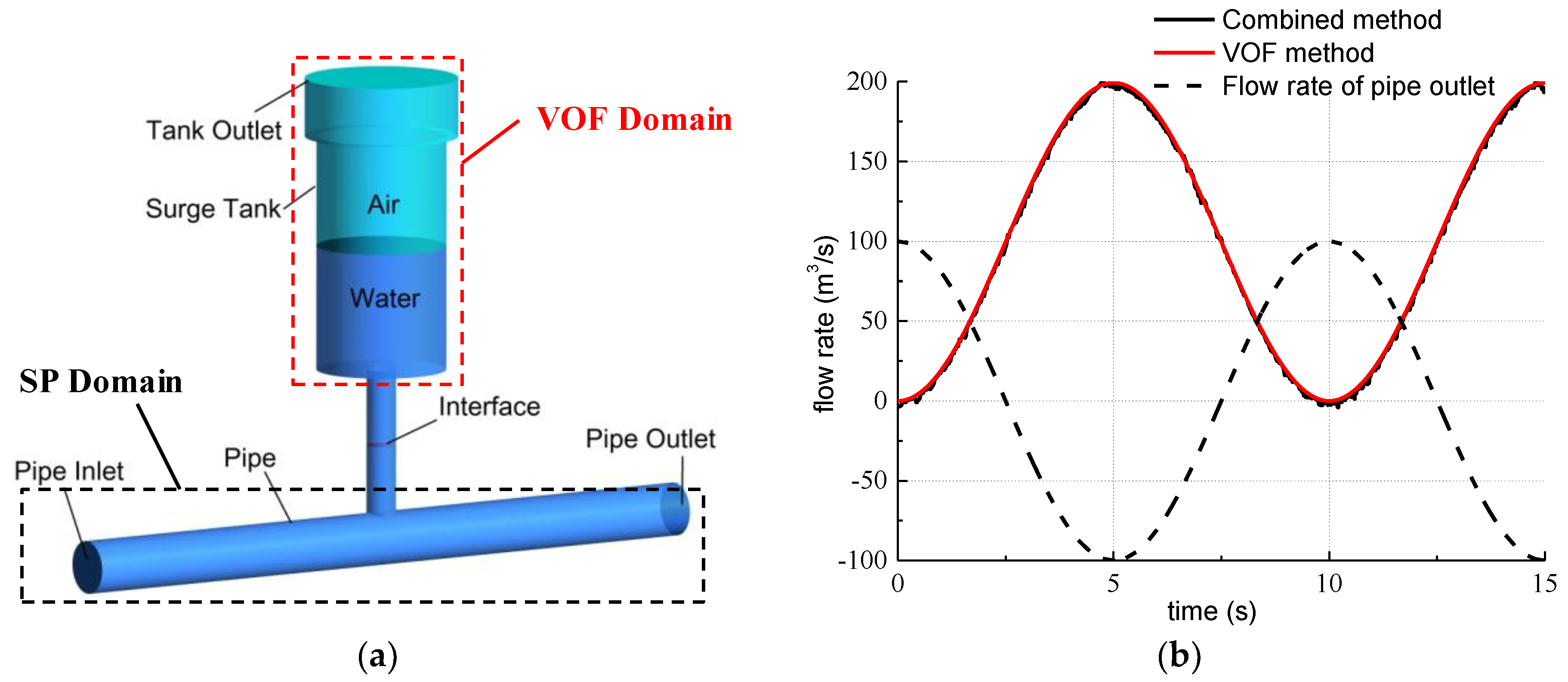
To verify the reliability and accuracy of the hybrid simulation method, a simplified model consisting of a surge tank and a portion of pipe was set up (Figure 1a), and one transient process with the same boundary conditions was simulated, which were defined as follows: (1) The tank outlet was opened to atmosphere, and its static pressure remained at zero. (2) The water flow rate at the pipe inlet was equal to 100 m3/s, and that at the pipe outlet varied with time (Figure 1b). The initial water volume in surge tank was initialized as Figure 1a. Finally, the flow rate across the interface of the hybrid method was compared with that of the single VOF method.
Flow rate values of the hybrid method agreed well with the VOF simulation results (Figure 1b), and the maximum relative error of flow rate was 1.32% when the time was equal to 5 s. In addition, the pumped storage power station was much bigger in volume than the surge tank, so the errors at other parts caused by the hybrid simulation method would be very small.
2.4. Algorithm of Power-off Transient Simulation
Algorithm routine of power-off transient simulation was implemented by a secondary developed and customized program basing on widely used CFD software, Fluent 6.3 (ANSYS, Canonsburg, PA, USA) and the algorithm routine diagram was described as follows (Figure 2):
3. Case Study
3.1. Geometry Model and Initial Parameters
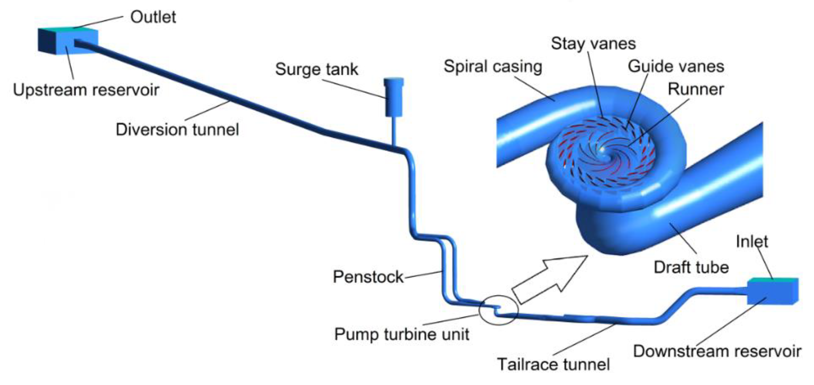
The pumped storage hydropower station involved in this simulation consists of an upstream reservoir, a diversion tunnel, surge tank, pump-turbine units, and so on, whose detailed structure was displayed in Figure 3. The length of diversion tunnel, penstock, and tailrace tunnel is 1260 m, 190 m, and 355 m, respectively, and the corresponding diameter is 9 m, 5.6 m, and 10 m. The specific speed of pump-turbine unit ns = 182 m·kW, and its runner outlet diameter D = 3.57 m, total unit moment of inertia J = 4,825,000 kg·m2. In addition, the pump-turbine unit has 20 stay vanes, 20 guide vanes and 9 runner blades. Some important parameters of initial condition are as follows: pumping lift = 205 m, unit flow rate Q0 = 139 m3/s, runner rotating speed n0 = 250 r/min, the initial torque M0 = −11.7 × 10⁶ N, guide vane opening angle γ = 23.75° (75% of fully opening), and input power P0 = 306 kW.
3.2. Grid Technology
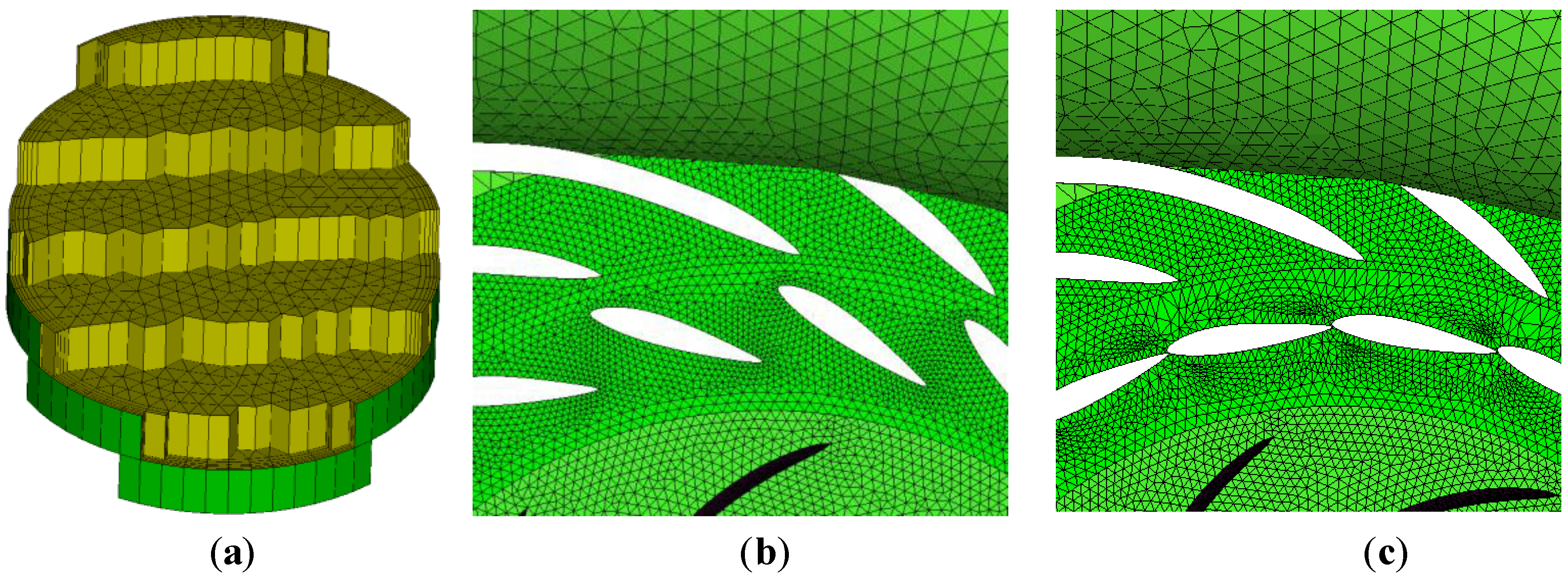
According to physical characteristics of different regions, we made different meshing schemes. Narrow prism grids were meshed in pipes, and tetrahedral grids were meshed at other places. We also performed the grid refinement for some places, such as the region near pipe wall, the runner and the guide vanes. Varying speed sliding mesh technology was used to transfer flow field parameters between runner zone and adjacent part passages, meanwhile, mesh rotating of guide vanes was resolved by dynamic mesh technology [34].
3.3. Equations Discretization and Boundary Condition
The governing equations of the hybrid SP-VOF method were discrete with finite volume method, and the first order implicit format was used for time item. For the single-phase model applied in pipes and unit, the second order format was used for pressure item, the second order upwind format for convection item, and Semi-implicit method for pressure linked equations-consistent (SIMPLEC) algorithm was chosen to obtain the coupling solution from velocity and pressure equations. For the VOF model in the surge tank, the PRESTO! Format was used for pressure item, the first order upwind format for momentum item and turbulent kinetic energy, and PISO algorithm for velocity–pressure coupling solution.
Due to small change of reservoir water level in the transient process, their inlet or outlet pressure value was assumed to be constant, according to their water depth, and the surge tank outlet was opened to atmosphere, which had a relative pressure that was equal to zero. We also set the roughness values of different passage walls: 2.55 mm for surge tank, diversion system, and tailrace system; 0.06 mm in the casing; 0.0016 mm on runner blades and vanes. In addition, runner rotate speed was calculated by Equation (8), and closing law of guide vanes was given by Equation (9).
where is the runner rotate speed, is resultant torque of the rotational system, is time step size, and is the change amount of guide vane opening.
3.4. Data Monitoring and Processing
In this study, for the assessment of this transient process, and some dynamic parameters, such as runner rotate speed n, pumping lift H, unit flow rate Q and torque M, are obtained and normalized and divided by corresponding parameters values under the initial condition. However, the surge tank flow rate Qst is normalized by initial unit flow, because its initial value is regarded as zero. In order to monitor variable regularities of static pressure, three measuring points were set in the pump-turbine passage. Point 1 was at the inlet section center of spiral case, point 2 was at the half height of trailing edge of guide vane, and point 3 was at the center of draft tube inlet.
4. Results and Discussion
4.1. Test Results of Grid and Time Dependency
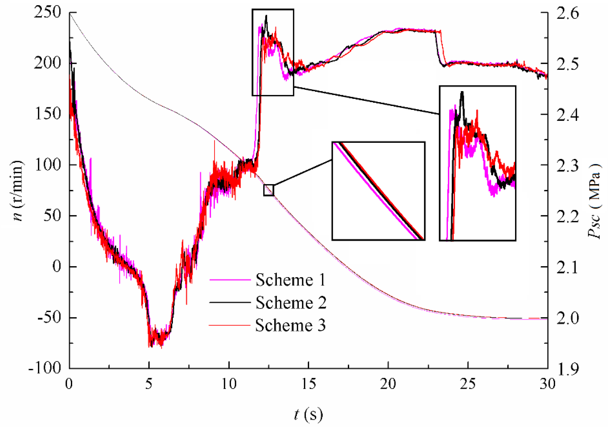
To eliminate influences caused by computational grids, three different meshing schemes are employed in the CFD simulation: the corresponding mesh grid size is about 2.5 million, 3.5 million, and 4.5 million respectively. The two parameters of pre-calculated results, namely unit rotate speed and static pressure of spiral casing inlet, were plotted in Figure 4. Though the two parameters’ overall varying tendency under the three meshing schemes is similar, the local details still retain slightly different, especially under the intense fluctuation region. Obviously, the curves of scheme 2 are closer to that of scheme 3 than that of scheme 1. Thus, scheme 2 was chosen based on the available computing power and subdivision scheme for each part of flow passage, as was listed in the Table 1. Finally, Figure 5 shows some details of the mesh in different regions of the PSH model.
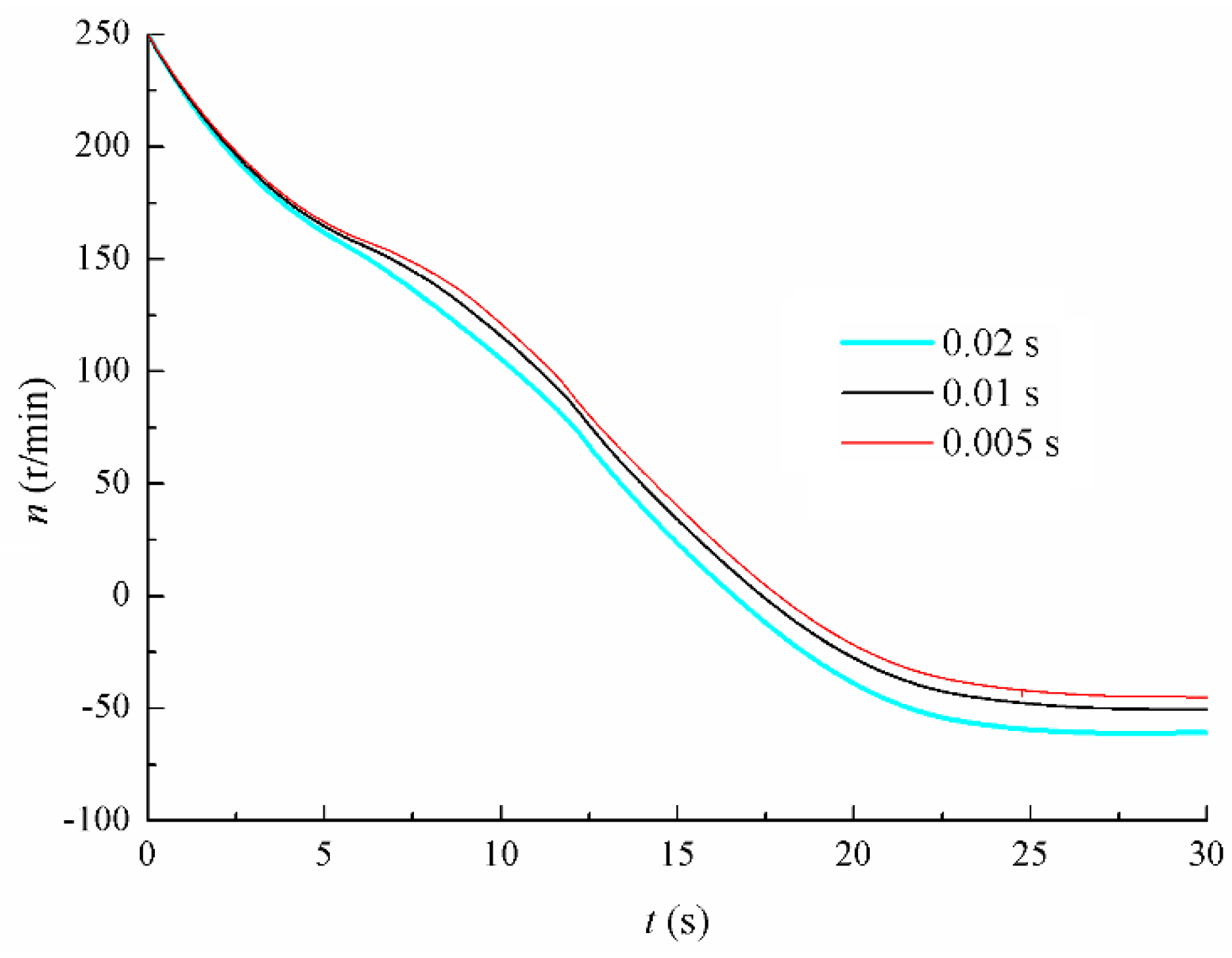
Similarly, different time step sizes also have influences on the unsteady numerical results of the transient parameters. Three different time step sizes were used to pre-compute: 0.02 s, 0.01 s, and 0.005 s, respectively. The corresponding results of runner rotating speed were described in Figure 6, and showed that the shorter time step led to the slower decreasing rotating speed and smaller runaway speed value. To obtain more detailed transient information, the 0.005 s time step size was adopted finally.
4.2. The Varying Law of Dynamic Characteristics Parameters
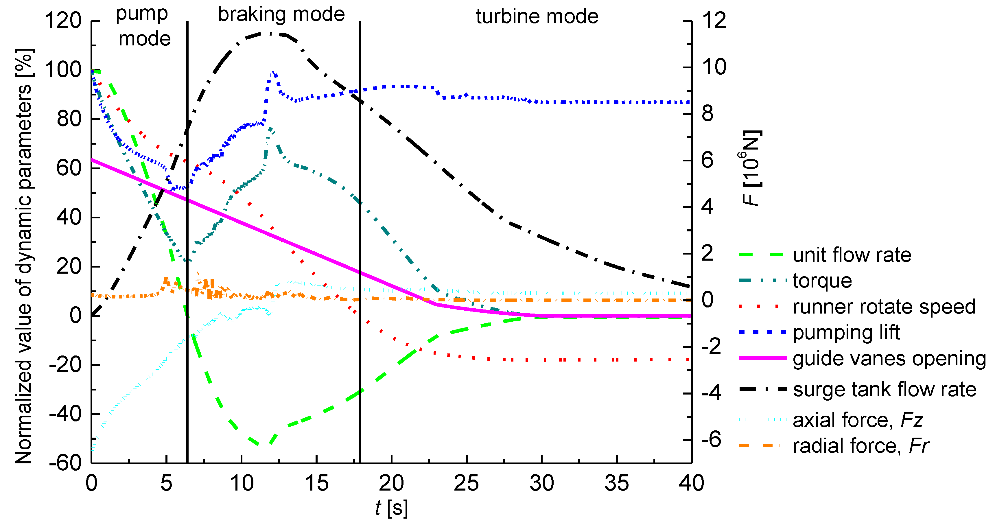
Once the transient process began, the PSH station would undergo pump mode, braking mode, and turbine mode in sequence (Figure 7). In the beginning period, unit flow rate Q, pumping lift H and torque M declined quickly with decreasing runner rotate speed n after power failure. Nevertheless, the surge tank flow rate Qst rose rapidly, and supplied water to the diversion tunnel due to its pressure decreasing. As time arrived at 6.4 s, unit flow rate Q was equal to 0, which indicated the end of pump mode. Meanwhile, pumping lift H and torque M reached the minimum values, and from then on, the unit was running in braking mode for 11.5 s. During this time, reversed flow rate Q, torque M, and pumping lift H had been increasing until t = 11.6 s, and then decreased slowly with guide vanes closed. It was noted that there were sharp turning points on the curves of Q, Qst, , and H at t = 11.6 s because of the water hammer effect, and more detailed discussion will be conducted later, combined with flow field characteristics. After t = 17.8 s, the unit entered into turbine mode marked as the unit rotating speed direction changed, and all dynamic parameters became stable gradually, except the small changes at t = 22.95 s for the variable closing law of guide vanes. At last, runner rotate speed got the maximum reversed value 43.8 r/min when the torque M was equal to approximately zero, and the lift H was lower than the initial one, of which the difference was approximate to the hydraulic loss of pipes in initial pump mode.
In this simulation of power-off transient process, surge tank always supplied water to diversion tunnel. Before t = 10.1 s, the water flow rate from the surge tank had been increasing until reaching the maximum value (112% of the unit flow rate). Then, the discharge of the surge tank decreased gradually due to the decline of the water level in the surge tank, and increased diversion tunnel pressure.
The dynamic loads on the runner affect the stability of the pump-turbine unit directly. The axial force Fz and radial force Fr acting on the runner were plotted in Figure 7. The absolute value of axial force Fz had been decreasing in pump mode and fluctuating in braking mode until the force direction changed at t = 11.6 s, when the reversed unit flow rate reached maximum value. Then, the axial force Fz jumped to the maximum reverse value of nearly 106 N suddenly, concurrently with the pumping lift and torque. By comparison, the variation of radial force Fr was smaller, but fluctuated at a higher frequency in the end stage of pump mode when the unit flow rate went down to the minimum.
4.3. Comparisons between Numerical and Experimental Results
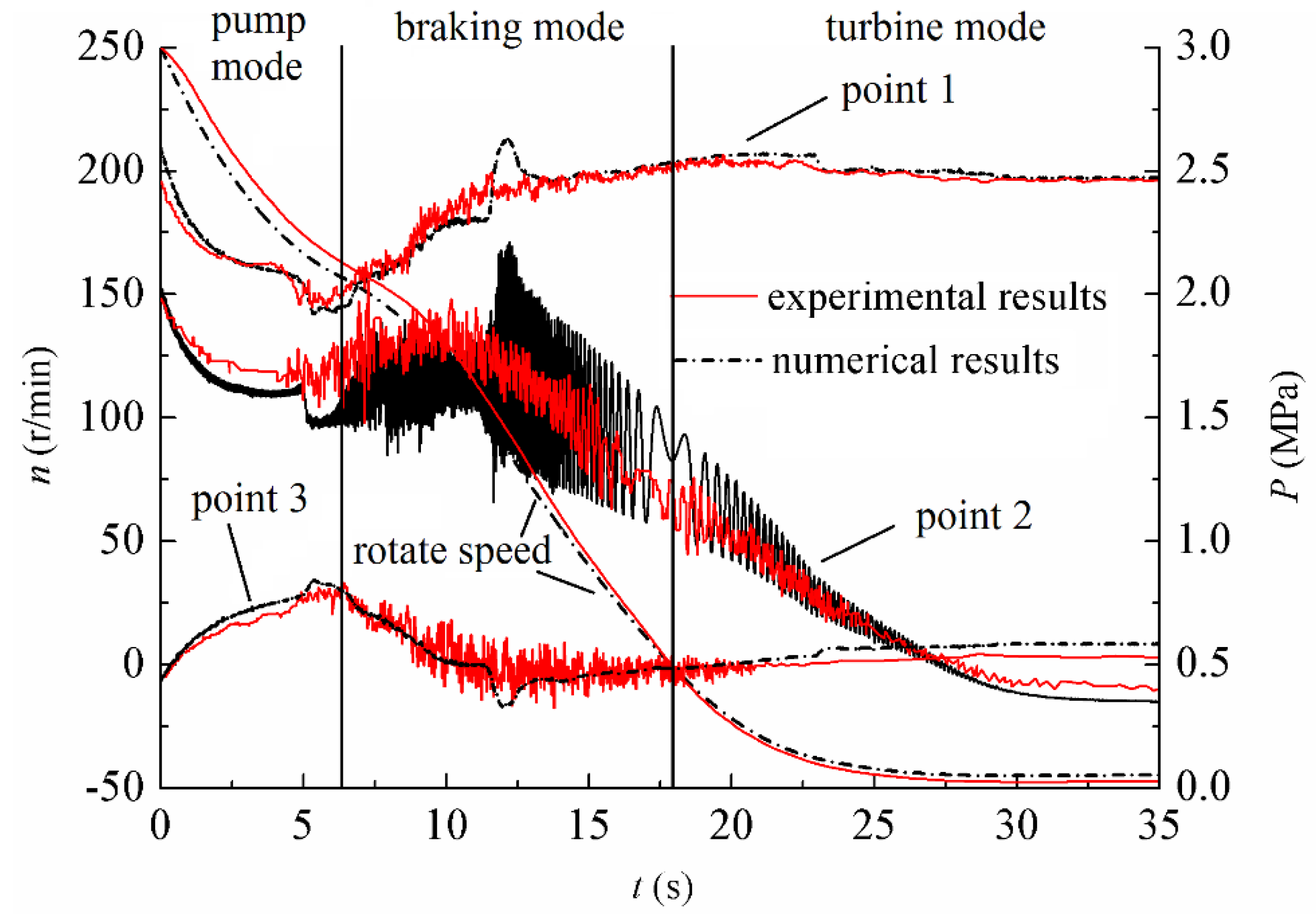
To verify the reliability and the accuracy of the power-off transient simulation, some numerical values, namely runner rotating speed and static pressure of measuring points (Figure 8), were compared with prototype test results (Figure 9).
The overall trends of numerical results agreed well with experimental ones, particularly under the pump and turbine conditions located on both sides of the figure. However, the rotating speed derived from numerical approach decreased a bit faster than experimental results, which may be due to that the moment of inertia value used in the numerical simulation was not exactly the same as the actual value. In addition, the pressure fluctuation characteristics between the two methods had significant discrepancy, especially when pump-turbine unit was operated in the braking mode. Compared with experimental data, the numerical results displayed the higher pressure amplitude at point 2, but lower amplitude at point 1 and point 3, besides the remarkable pressure jump at t = 11.6 s. The three possible explanations for their differences could be deduced as follows: (1) they have different acquisition frequency; (2) some kinds of vortexes or cavitation could not be fully simulated due to the limitations of the using numerical model and grid size, so that their contributions to the pressure fluctuation could not be reflected; (3) the measured pressure data from field test may include the vibration signals of the unit.
Then, the more details of the static pressure variation obtained by the numerical method would be described and explained. The static pressure of point 1 at the spiral casing had been declining from 2.6 MPa to 1.9 MPa near the end of pump mode, due to pumping energy reduction. Once entering the braking mode, it showed an uptrend and ascended to 2.63 MPa suddenly, when the maximum reversed flow rate appeared. Since the guide vanes’ closing speed changed, it stepped to a lower level at t = 23 s. In pump mode, the variation law of static pressure at point 2 was same as that of point 1, but presented strong pulsation in braking mode, of which the frequency was related with the runner rotate speed, and the maximum amplitude, equal to about 1 MPa, was recorded when the maximum reversed flow rate appeared, too. In the whole process, the variation range of static pressure at point 2 was also much bigger than that of other two points, decreasing from 2 MPa to 0.35 MPa. The curve of point 3 showed that static pressure in draft tube had an opposite variation trend towards that in the spiral casing, which caused the decrease of pumping lift H. In summary, the static pressure during power-off transient process had a complex variation, not only related with position, but also affected by dynamic parameters, such as runner rotate speed, unit flow rate, and guide vanes opening. So the visualization of transient flow field can help to increase our understanding of hydrodynamic mechanism.
4.4. Transient Flow Fields
Obviously, the flow field in pumped storage power station passage will take on different features during power-off transient process, which is the intrinsic factor leading to variations of dynamic parameters. In the following, transient flow fields of different parts at some critical moments are plotted and visualized for analysis.
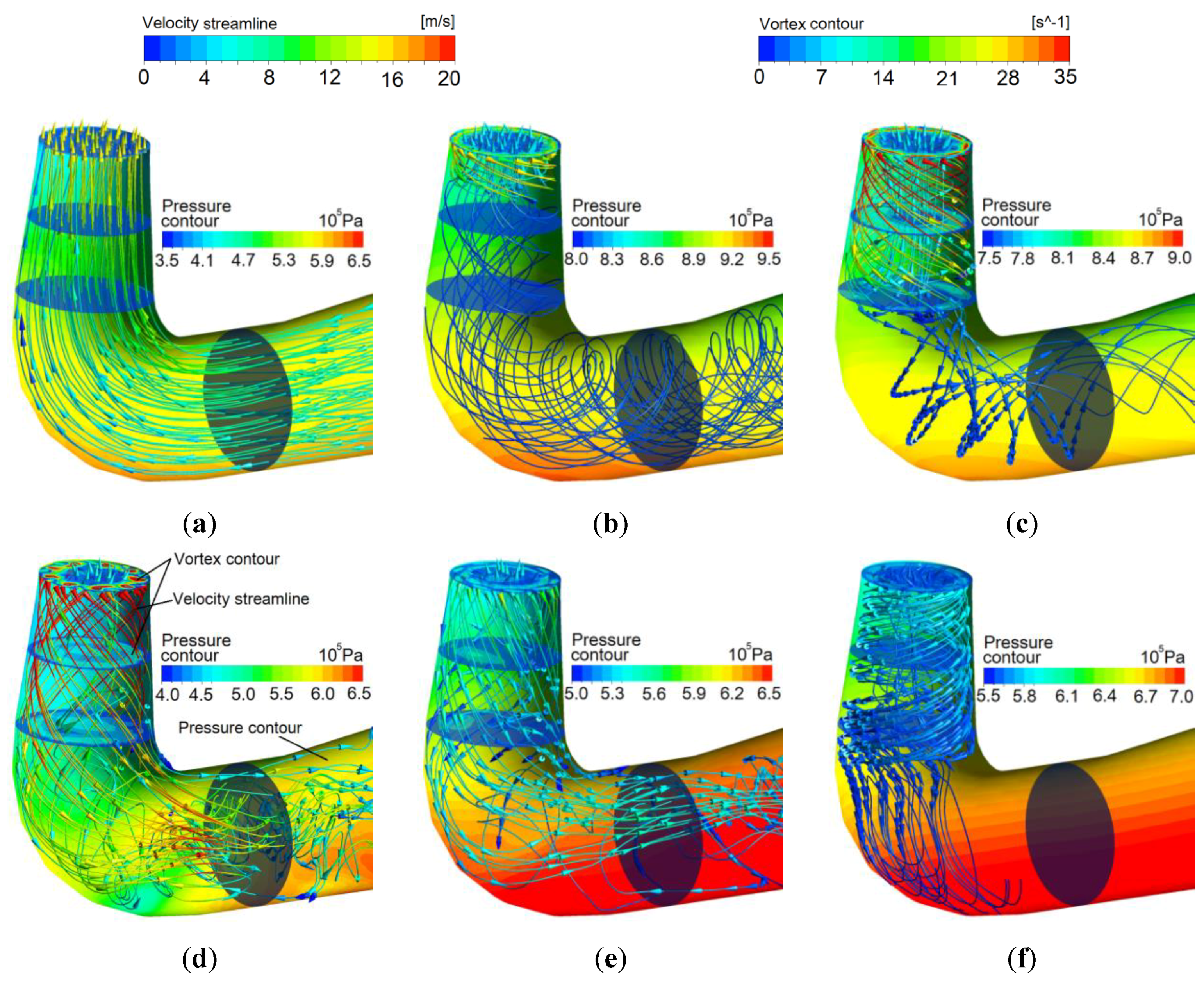
Figure 10 displayed flow fields between spiral casing and guide vanes at different moments. The initial condition had a perfect performance with water flowing upstream smoothly (Figure 10a). When pump rotational speed dropped, unit flow rate and static pressure decreased during the pump mode. When the unit just changed its flow direction at t = 6.5 s, the water in the region flowed slowly and disorderly, with minimum static pressure (Figure 10b). Then, in braking mode at t = 12 s, the water flowed downstream smoothly in the region, and static pressure in the spiral casing achieved a peak value when the reverse discharge reached maximum value (Figure 10c). After the guide vanes were closed completely, the flow pattern in the channels between stay vanes became disorder and the circumfluent flow with small velocity between the stay vanes and guide vanes emerged, due to the previous flow inertia (Figure 10d).
The runner is the most important part of a pump-turbine unit [35], which not only decides steady state performance, but also has great influence on transient characteristics. Obviously, there was no vortex or flow separation in the runner region under the beginning condition (Figure 11a). Once power-off happened, flow configuration in the runner would undergo very complex and unsteady change. When the runner rotate speed reduced 40% at t = 6.5 s, low speed vortex flow appeared at the inlet of runner due to the loss of pumping function for water (Figure 11b). Since then, water changed flow direction, but direction of runner rotate speed remained the same as initial one. As a result, there were jets towards the front of blade, leading to high static pressure on front blade and negative pressure on the middle part. Vortex flow also became stronger, not only behind the leading edge of the blade, but also near the trail of guide vanes (Figure 11c), which could be the typical flow characteristics in braking mode. In addition, the amplitude of pressure fluctuation at point 2 was determined by varying rotor–stator interactions between runner blades and guide vanes. With guide vanes closed, as well as the variations of both reversed flow rate and rotating speed, the angle between jets flowing from guide vanes and blade chord line, the so-called angle of attack, changed from acute angle to right angle, and continued to increase from right angle to obtuse angle, observed from Figure 11c–e. During the first stage, the vector vertical component of jets towards blade strengthened gradually, so that the drag torque exhibited corresponding increase. However, when the angle of attack reached nearly 90°, the maximum value of pressure on the blade convex face occurred, with a large vortex formed among the inlet of blade passages (Figure 11d), which caused water flow to be clogged suddenly, and led to water hammer resulting in sharp turning points at t = 11.8 s on curves plotted in Figure 7. While entering into the turbine mode, runner was rotating reversely, pushed by water. At t = 33 s, although the complete closure of guide vanes broke the connection between runner and spiral casing, the runner still maintained runaway condition for a short time with no difference of static pressure on both side of runner blades (Figure 11f). Then, the unit rotating speed would continue to decline because of the effects of drag torque, until it was forced to brake.
Though geometric structure of draft tube is simple, its transient flow pattern changed significantly since it connected with the runner directly. According to Figure 12a, initial flow fields in the draft tube were harmonious before the transient process happened. With the runner lifting capacity decreasing, static pressure of the draft tube inlet had been increasing in pump mode, due to the effect of water hammer formed by the flow rate difference between the inlet and outlet of the runner. After entering into braking mode, the water would flow into the draft tube via the outside lane of the inlet, and flow back to the runner through the inlet center. When reversed flow rate reached maximum near t = 12 s, the flow regime became very disordered (Figure 12d), and the water flowed into draft tube choppily with 9 branched vortexes induced by the runner, and the static pressure in the entrance center of draft tube is lowest and asymmetrical. When the unit entered turbine mode, the flow became much gentler than that in braking mode. After t = 30 s, unit flux was equal to zero again, but the flow in draft tube was driven by the runner and whirled, and static pressure took on layered distribution, due to gravity effect (Figure 12f).
5. Conclusions
The 3D SP-VOF hybrid model is an effective method to study the transient process of the whole PSH station flow system in pump mode. During the power-off process, the hydraulic performance of the pump-turbine changed significantly as well as its inner flow configurations while undergoing pump mode, braking mode, and turbine mode, sequentially. Especially in the braking mode, the flow is the most unstable with the great pressure pulsation. The flow was blocked by the strong vortexes in the runner blade channels at t = 11.6 s under the 40% of the rated rotate speed and 34% of the initial guide blade opening, which induced a notable water hammer and resulted in the sudden changes of the dynamic parameters. The axial force on the runner is not larger than the initial value during the transient process, while the radial force will fluctuate irregularly in braking mode. The pressure fluctuation between guide vanes and runner is the most intense, whose frequency is determined by runner rotate speed and amplitude, and is related to the dynamic rotor–stator interactions between the guide vanes and runner blades.
Future studies should establish a high-precision and compressible 3D numerical model that considers the effects of the water density change on the results during the transient process [36,37], and the calculation conditions should be increased so that the transient process of power-off transient process in PSH could be more precisely and fully investigated.
Acknowledgments
The study was supported by Open Research Fund Program of State Key Laboratory of Water Resource and Hydropower Engineering Science (2015SDG04) and the Key Program of National Science Foundation of China (No. 51339005). The support of College of Energy and Electrical, Hohai University, China is also gratefully acknowledged. The study was also supported by the Fundamental Research Funds for the Central Universities (2015B34314). The financial support provided by the Chinese Scholarship Council (No. 201606710029) is gratefully acknowledged.
Author Contributions
Daqing Zhou and Huixing Chen analyzed the numerical results and wrote the paper; Languo Zhang designed the 3D SP-VOF hybrid numerical approach and performed the numerical simulation.
Conflicts of Interest
The authors declare no conflict of interest.
Nomenclature
| D | Runner outlet diameter | m |
| F | External body force | N |
| Fz | Axial force | N |
| Fr | Radial force | N |
| g | Gravitational body force | m/s2 |
| H0 | Initial pumping lift | m |
| I | Unit tensor | - |
| J | Total unit moment of inertia | kg·m2 |
| M | Resultant torque of the rotational system | N |
| M0 | Initial torque | N |
| Mass transfer from water to air | kg | |
| Mass transfer from air to water | kg | |
| n | Runner rotating speed | r/min |
| n0 | Initial runner rotating speed | r/min |
| ns | Specific speed of pump-turbine unit | m·kW |
| p | Static pressure | MPa |
| P0 | Initial input power | kW |
| Psc | Static pressure of spiral casing inlet | MPa |
| Q | Unit flow rate | m3/s |
| Q0 | Initial unit flow rate | m3/s |
| Qst | Surge tank flow rate | m3/s |
| Source term | kg/(m3·s) | |
| t | Time | s |
| u | Velocity | m/s |
| Runner outlet rotating speed | rad/s | |
| Volume fraction of water in a cell | - | |
| Volume fraction of air in a cell | - | |
| Relaxation factor | - | |
| ρ | Density of fluid | kg/m3 |
| μ | Molecular viscosity | Pa·s |
| γ | Initial guide vane opening angle | ° |
| Stress tensor | - | |
| Time step size | s | |
| Changing amount of guide vane opening | ° |
Abbreviations
| 1D | One dimensional |
| 3D | Three dimensional |
| CFD | Computational fluid dynamics |
| MOC | Method of characteristics |
| PISO | Pressure implicit with splitting of operators |
| PSH | Pumped storage hydropower |
| SIMPLEC | Semi-implicit method for pressure linked equations-consistent |
| SP | Single-phase |
| UDF | User defined function |
| VOF | Volume of fluid |
References
- Benjamin, K.S. The intermittency of wind, solar and renewable electricity generators: Technical barrier or rhetorical excuse? Util. Policy 2009, 17, 288–296. [Google Scholar]
- Cheng, C.; Cheng, X.; Shen, J.; Wu, X. Short-term peak shaving operation for multiple power grids with pumped storage power plants. Int. J. Electr. Power Energy Syst. 2015, 67, 570–581. [Google Scholar] [CrossRef]
- Pérez-Díaz, J.I.; Chazarra, M.; García-González, J.; Cavazzini, G.; Stoppato, A. Trends and challenges in the operation of pumped-storage hydropower plants. Renew. Sustain. Energy Rev. 2015, 44, 767–784. [Google Scholar] [CrossRef]
- Zeng, M.; Zhang, K.; Liu, D. Overall review of pumped-hydro energy storage in China: Status quo, operation mechanism and policy barriers. Renew. Sustain. Energy Rev. 2013, 17, 35–43. [Google Scholar]
- Widmer, C.; Staubli, T.; Ledergerber, N. Unstable characteristics and rotating stall in turbine brake operation of pump-turbines. J. Fluids Eng. 2011, 133, 041101. [Google Scholar] [CrossRef]
- Hasmatuchi, V.; Farhat, M.; Roth, S.; Botero, F.; Avellan, F. Experimental evidence of rotating stall in a pump-turbine at off-design conditions in generating mode. J. Fluids Eng. 2011, 133, 051104. [Google Scholar] [CrossRef]
- Hasmatuchi, V. Hydrodynamics of a Pump-Turbine Operating at Off-Design Conditions in Generating Mode. Ph.D. Thesis, École Polytechnique Fédérale de Lausanne (EPFL), Lausanne, Switzerland, 2012. [Google Scholar]
- Liu, J.; Liu, S.; Sun, Y.; Wu, Y.; Wang, L. Three dimensional flow simulation of load rejection of a prototype pump-turbine. Eng. Comput. 2013, 29, 417–426. [Google Scholar]
- Thanapandi, P.; Prasad, R. Centrifugal pump transient characteristics and analysis using the method of characteristics. Int. J. Mech. Sci. 1995, 37, 77–89. [Google Scholar] [CrossRef]
- Afshar, M.H.; Rohani, M.; Taheri, R. Simulation of transient flow in pipe line systems due to load rejection and load acceptance by hydroelectric power plants. Int. J. Mech. Sci. 2010, 52, 103–115. [Google Scholar] [CrossRef]
- Wan, W.; Huang, W. Investigation on complete characteristics and hydraulic transient of centrifugal pump. J. Mech. Sci. Technol. 2011, 25, 2583–2590. [Google Scholar] [CrossRef]
- Zhang, J.; Lu, W.; Fan, B.; Hu, J. The influence of layout of water conveyance system on the hydraulic transients of pump-turbines load successive rejection in pumped storage station. J. Hydroelectr. Eng. 2008, 27, 158–162. (In Chinese) [Google Scholar]
- Zhou, J.; Xu, Y.; Zheng, Y.; Zhang, Y. Optimization of guide vane closing schemes of pumped storage hydro unit an enhanced multi-objective gravitational search algorithm. Energies 2017, 10, 911. [Google Scholar] [CrossRef]
- Li, Z.; Bi, H.; Karney, B.; Wang, Z.; Yao, Z. Three-dimensional transient simulation of a prototype pump-turbine during normal turbine shutdown. J. Hydraul. Res. 2017, 55, 520–537. [Google Scholar]
- Gajic, A. Steady and Transient Regimes in Hydropower Plants; IOP Conference Series: Materials Science and Engineering; IOP Publishing: Bristol, UK, 2013; Volume 52. [Google Scholar]
- Yang, W.; Wu, Y.; Liu, S. An optimization method on runner blades in bulb turbine based on CFD analysis. Sci. China Technol. Sci. 2011, 54, 338–344. [Google Scholar] [CrossRef]
- Litfin, O.; Mohr, C.; Haddad, K.; Epple, P.; Semel, M.; Becker, K.; Klein, H.; Delgado, A. CFD computation, analysis and design of a two-bladed wastewater pump. In Proceedings of the ASME 2011 International Mechanical Engineering Congress & Exposition, Denver, CO, USA, 11–17 November 2011; p. 64195. [Google Scholar]
- Sedlar, M.; Sputa, O.; Komarek, M. CFD analysis of cavitation phenomena in mixed-flow pump. Int. J. Fluid Mach. Syst. 2012, 5, 18–29. [Google Scholar] [CrossRef]
- Xia, L.; Cheng, Y.; Zhou, D. 3-D simulation of transient flow patterns in a corridor-shaped air-cushion surge chamber based on computational fluid dynamics. J. Hydrodyn. Ser. B 2013, 25, 249–257. [Google Scholar] [CrossRef]
- Nicolle, J.; Morissette, J.F.; Giroux, A.M. Transient CFD Simulation of a Francis Turbine Startup; IOP Conference Series: Earth and Environmental Science; IOP Publishing: Bristol, UK, 2012; Volume 15. [Google Scholar]
- Zhou, D.; Wu, Y.; Liu, S. Three-dimensional CFD simulation of the runaway transients of a propeller turbine model. J. Hydraul. Eng. 2010, 41, 233–238. [Google Scholar]
- Cherny, S.; Chirkov, D.; Bannikov, D.; Lapin, V.; Skorospelov, V.; Eshkumova, I.; Avdushenko, A. 3D Numerical Simulation of Transient Processes in Hydraulic Turbines; IOP Conference Series: Earth and Environmental Science; IOP Publishing: Bristol, UK, 2010; Volume 12. [Google Scholar]
- Huang, W.; Fan, H.; Chen, N. Transient Simulation of Hydropower Station with Consideration of Three-Dimensional Unsteady Flow in Turbine; IOP Conference Series: Earth and Environmental Science; IOP Publishing: Bristol, UK, 2012; Volume 15. [Google Scholar]
- Yang, S.; Chen, X.; Wu, D.; Yan, P. Dynamic analysis of the pump system based on MOC–CFD coupled method. Ann. Nucl. Energy 2015, 78, 60–69. [Google Scholar] [CrossRef]
- Zhang, X.; Cheng, Y.; Yang, J.; Xia, L.; Lai, X. Simulation of the load rejection transient process of a Francis turbine by using a 1-D-3-D coupling approach. J. Hydrodyn. Ser. B 2014, 26, 715–724. [Google Scholar] [CrossRef]
- Liu, J.; Liu, S.; Sun, Y.; Jiao, L.; Wu, Y.; Wang, L. Three-dimensional flow simulation of transient power interruption process of a prototype pump-turbine at pump mode. J. Mech. Sci. Technol. 2013, 27, 1305–1312. [Google Scholar] [CrossRef]
- Li, Y.; Song, G.; Yan, Y. Transient hydrodynamic analysis of the transition process of bulb hydraulic turbine. Adv. Eng. Softw. 2015, 90, 152–158. [Google Scholar] [CrossRef]
- Mao, X.; Monte, A.D.; Benini, E.; Zheng, Y. Numerical study on the internal flow field of a reversible turbine during continuous guide vane closing. Energies 2017, 10, 988. [Google Scholar] [CrossRef]
- Luo, X.; Li, W.; Feng, J.; Zhu, G. Simulation of runaway transient characteristics of tubular turbine based on CFX secondary development. Trans. Chin. Soc. Agric. Eng. 2017, 33, 97–103. [Google Scholar]
- Zhou, L.; Liu, D.; Ou, C. Simulation of flow transients in a water filling pipe containing entrapped air pocket with VOF model. Eng. Appl. Comput. Fluid Mech. 2011, 5, 127–140. [Google Scholar] [CrossRef]
- Guo, L.; Liu, Z.; Geng, J.; Li, D.; Du, G. Numerical study of flow fluctuation attenuation performance of a surge tank. J. Hydrodyn. Ser. B 2013, 25, 938–943. [Google Scholar] [CrossRef]
- Hirt, C.W.; Nichols, B.D. Volume of fluid (VOF) method for the dynamics of free boundaries. J. Comput. Phys. 1981, 39, 201–225. [Google Scholar] [CrossRef]
- Shih, T.-H.; Liou, W.W.; Shabbir, A.; Yang, Z.; Zhu, J. A New k-ɛ Eddy-Viscosity Model for High Reynolds Number Turbulent Flows—Model Development and Validation. Comput. Fluids. 1995, 24, 227–238. [Google Scholar] [CrossRef]
- Murayama, M.; Nakahashi, K.; Matsushima, K. Unstructured Dynamic Mesh for Large Movement and Deformation. In Proceedings of the 40th Aerospace Sciences Meeting and Exhibit, Reno, NV, USA, 14–17 January 2002; p. AIAA-2002-0122. [Google Scholar]
- Zheng, J.; Liu, W.; Fu, Z.; Shi, Q. The Hydraulic Design of Pump Turbine for Xianyou Pumped Storage Power Station; IOP Conference Series: Earth and Environmental Science; IOP Publishing: Bristol, UK, 2012; Volume 15. [Google Scholar]
- Meniconi, S.; Brunone, B.; Ferrante, M. In-line pipe device checking by short-period analysis of transient tests. J. Hydraul. Eng. 2011, 137, 713–722. [Google Scholar] [CrossRef]
- Stevanovic, V.; Studovic, M.; Bratic, A. Simulation and analysis of a main steam line transient with isolation valves closure and subsequent pipe break. Int. J. Numer. Methods Heat Fluid Flow 1994, 4, 387–398. [Google Scholar] [CrossRef]
Figure 1.
(a) Simplified pipe and surge tank model; (b) The flow rate across the shared interface obtained by two different methods and the flow rate of pipe outlet varied with the time.
Figure 1.
(a) Simplified pipe and surge tank model; (b) The flow rate across the shared interface obtained by two different methods and the flow rate of pipe outlet varied with the time.

Figure 2.
Algorithm routines of pumped storage hydropower (PSH) power-off transient simulation.
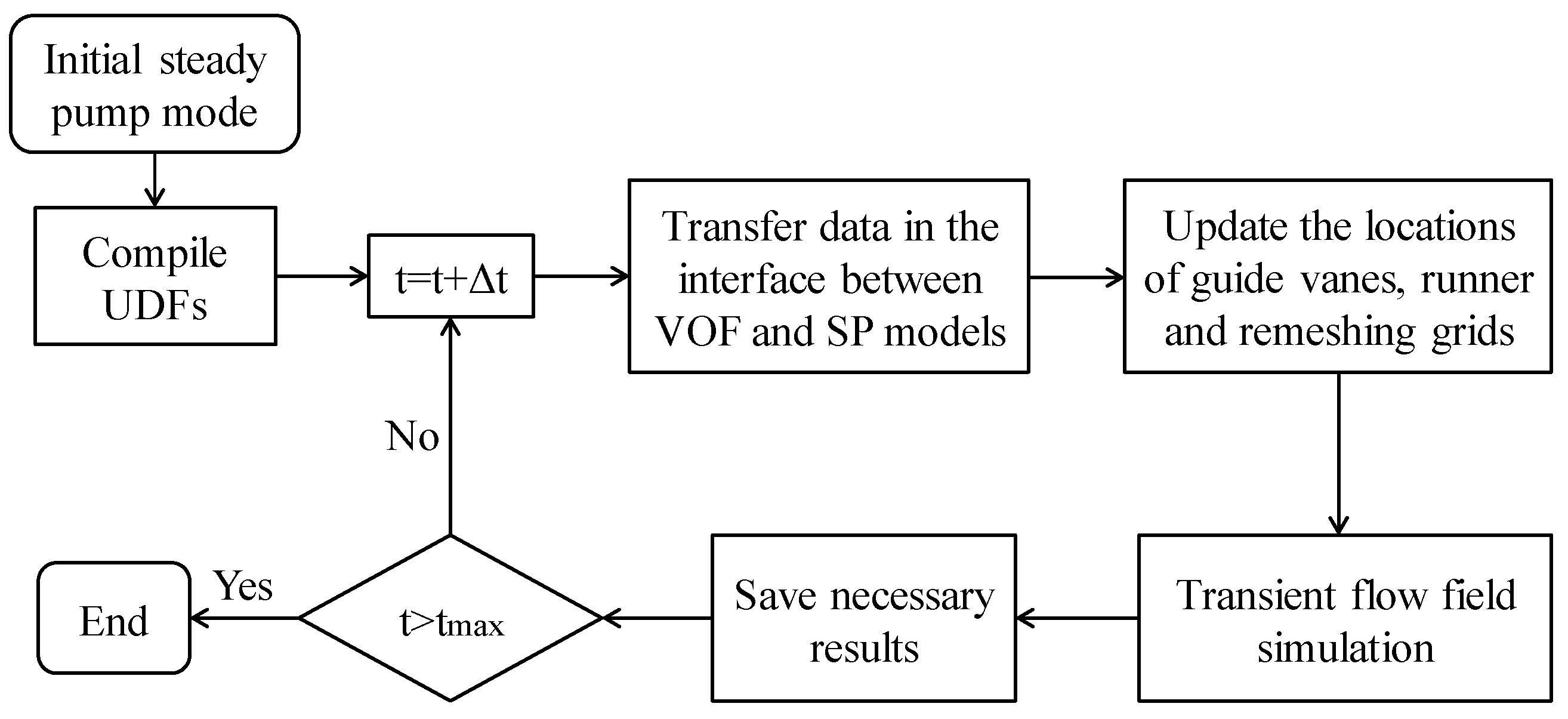
Figure 3.
The whole flow system of the pumped storage power station.

Figure 4.
Pre-calculated results of different meshing schemes.

Figure 5.
(a) Local section of pipeline grid; (b) Grid near the guide vane in the initial time; (c) Grid near the guide vane at full closed time.
Figure 5.
(a) Local section of pipeline grid; (b) Grid near the guide vane in the initial time; (c) Grid near the guide vane at full closed time.

Figure 6.
Pre-calculated results of different time step schemes.

Figure 7.
The left Y-axis is shared by normalized value of dynamic parameters variations with time; the right Y-axis is shared by axial and radial force on runner vs. time.
Figure 7.
The left Y-axis is shared by normalized value of dynamic parameters variations with time; the right Y-axis is shared by axial and radial force on runner vs. time.

Figure 8.
Measuring points of static pressure in the passage.
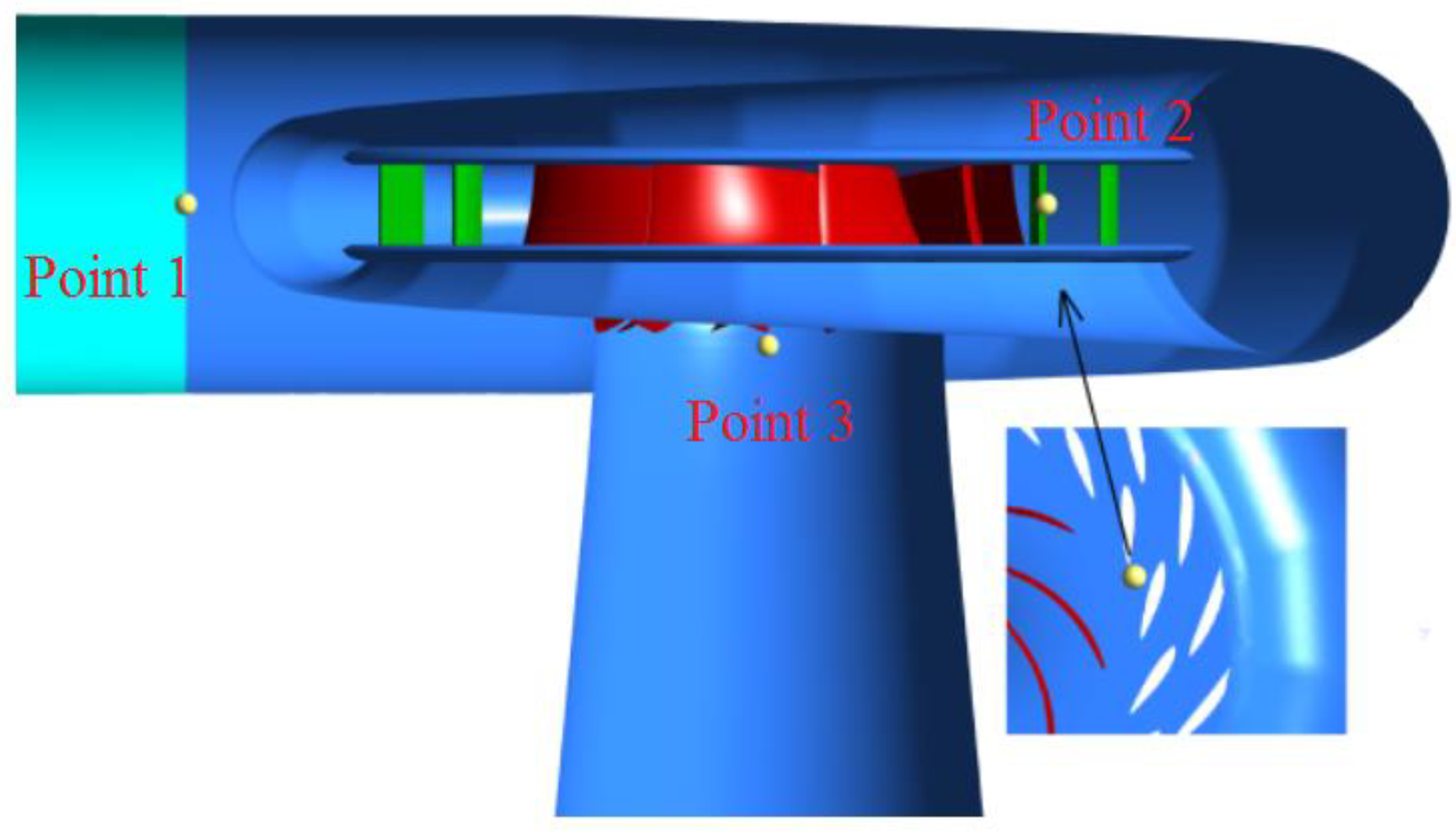
Figure 9.
Curves of experiment and simulation results.

Figure 10.
Flow fields between spiral case and guide vanes at different moments. (a) t = 0 s; (b) t = 6.5 s; (c) t = 12 s; (d) t = 33 s.
Figure 10.
Flow fields between spiral case and guide vanes at different moments. (a) t = 0 s; (b) t = 6.5 s; (c) t = 12 s; (d) t = 33 s.
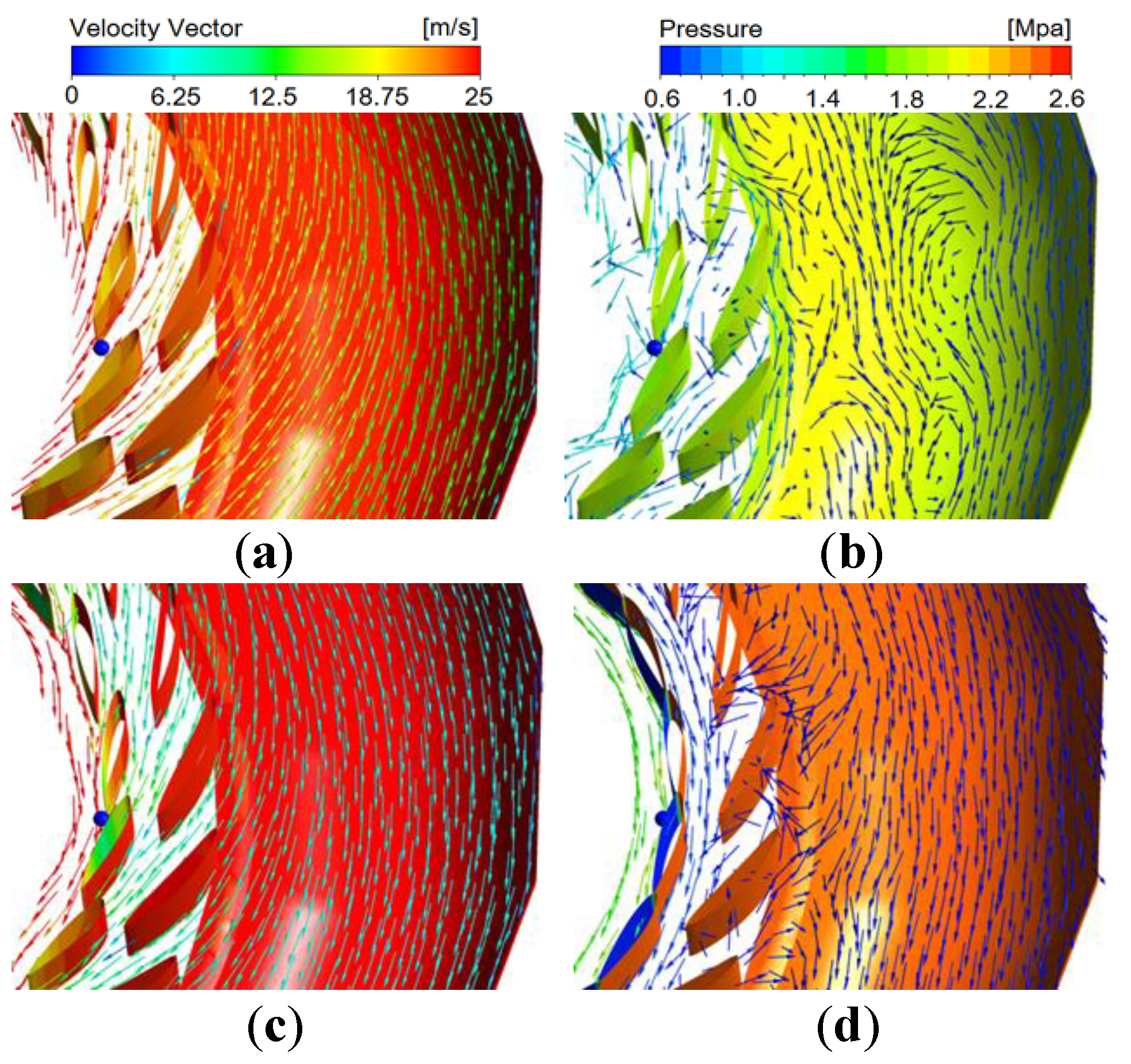
Figure 11.
Flow fields in runner at different moments. (a) t = 0 s; (b) t = 6.5 s; (c) t = 10 s; (d) t = 12 s; (e) t = 20 s; (f) t = 33 s.
Figure 11.
Flow fields in runner at different moments. (a) t = 0 s; (b) t = 6.5 s; (c) t = 10 s; (d) t = 12 s; (e) t = 20 s; (f) t = 33 s.
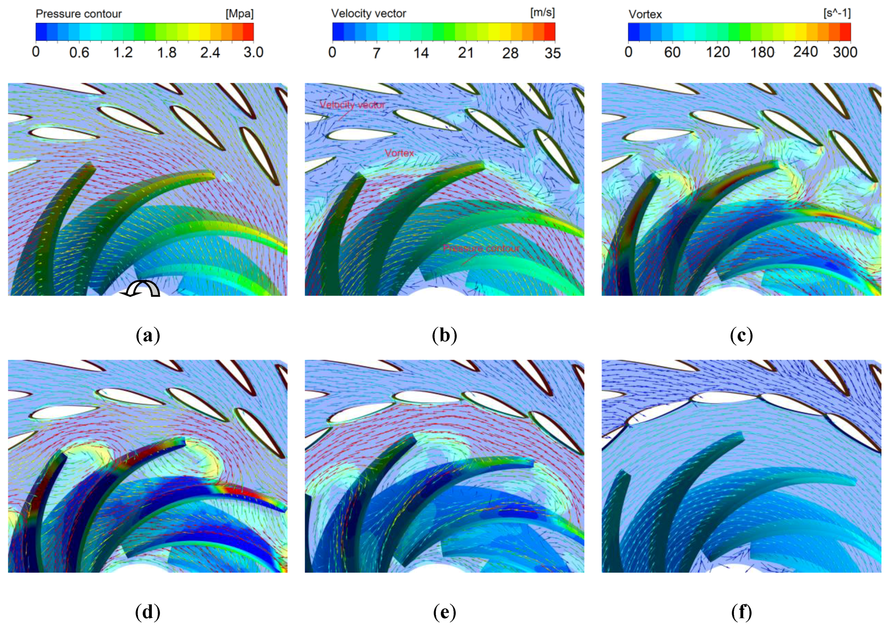
Figure 12.
Flow fields in draft tube at different moments. (a) t = 0 s; (b) t = 6 s; (c) t = 7 s; (d) t = 12 s; (e) t = 20 s; (f) t = 33 s.
Figure 12.
Flow fields in draft tube at different moments. (a) t = 0 s; (b) t = 6 s; (c) t = 7 s; (d) t = 12 s; (e) t = 20 s; (f) t = 33 s.


Table 1.
Mesh subdivision schemes of the PSH station.
| Passage | Mesh Elements Type | Mesh Numbers |
|---|---|---|
| Upstream reservoir | Tet/Hybrid | 93,814 |
| Diversion system | Hex/Wedge | 480,516 |
| Surge tank | Hex/Wedge | 382,608 |
| Casing | Tet/Hybrid | 435,415 |
| Stay/guide vane | Tet/Hybrid | 795,432 |
| Runner | Tet/Hybrid | 714,785 |
| Draft tube | Tet/Hybrid | 560,718 |
| Tailrace system | Hex/Wedge | 410,845 |
| Downstream reservoir | Tet/Hybrid | 93,814 |
© 2018 by the authors. Licensee MDPI, Basel, Switzerland. This article is an open access article distributed under the terms and conditions of the Creative Commons Attribution (CC BY) license (http://creativecommons.org/licenses/by/4.0/).
Share and Cite
MDPI and ACS Style
Zhou, D.; Chen, H.; Zhang, L. Investigation of Pumped Storage Hydropower Power-Off Transient Process Using 3D Numerical Simulation Based on SP-VOF Hybrid Model. Energies 2018, 11, 1020. https://doi.org/10.3390/en11041020
AMA Style
Zhou D, Chen H, Zhang L. Investigation of Pumped Storage Hydropower Power-Off Transient Process Using 3D Numerical Simulation Based on SP-VOF Hybrid Model. Energies. 2018; 11(4):1020. https://doi.org/10.3390/en11041020
Chicago/Turabian StyleZhou, Daqing, Huixiang Chen, and Languo Zhang. 2018. "Investigation of Pumped Storage Hydropower Power-Off Transient Process Using 3D Numerical Simulation Based on SP-VOF Hybrid Model" Energies 11, no. 4: 1020. https://doi.org/10.3390/en11041020
Note that from the first issue of 2016, this journal uses article numbers instead of page numbers. See further details here.