Current Density Distribution Mapping in PEM Fuel Cells as An Instrument for Operational Measurements

Abstract

A newly developed measurement system for current density distribution mapping has enabled a new approach for operational measurements in proton exchange membrane fuel cells (PEMFC). Taking into account previously constructed measurement systems, a method based on a multi layer printed circuit board was chosen for the development of the new system. This type of system consists of a sensor, a special electronic device and the control and visualization PC. For the acquisition of the current density distribution values, a sensor device was designed and installed within a multilayer printed circuit board with integrated shunt resistors. Varying shunt values can be taken into consideration with a newly developed and evaluated calibration method. The sensor device was integrated in a PEM fuel cell stack to prove the functionality of the whole measurement system. A software application was implemented to visualize and save the measurement values. Its functionality was verified by operational measurements within a PEMFC system. Measurement accuracy and possible negative reactions of the sensor device during PEMFC operation are discussed in detail in this paper. The developed system enables operational measurements for different operating phases of PEM fuel cells. Additionally, this can be seen as a basis for new opportunities of optimization for fuel cell design and operation modes.

1. Introduction

Criteria like costs, power- and energy density, efficiency, long-term behavior and integration options for existing systems are important factors for an economic and efficient application of PEM fuel cells. Starting points for improving PEMFC technology are basic studies [1,2,3] about processes and effects as well as technical progress in the field of stack and system optimisation. The electrochemical properties of a PEMFC are under particular consideration because they produce current density inhomogeneities due to varying reactions and activities in the active cell area. The inhomogeneity of the current density is also influenced by parameters like temperature and humidity of the membrane and has a fundamental influence on the life cycle of a fuel cell, which is complicated to model and to measure. A determination of current density distributions (CDD) inside the cells can accordingly supply information about the mentioned processes.

Various types of investigation can be used to analyse the system behavior of PEM fuel. Some approved methods are the electrochemical impedance spectroscopy (EIS) [4], infrared thermography [5,6], neutron radiography for an investigation of water accumulation [7] and current interruptions to determine the membrane and diffusion over-potential [1,8]. However, the mentioned methods require adapted cell configurations and more or less extensive measurement arrangements. Moreover, these methods for development and research do not deliver sufficient data for performance and operational measurements. Therefore, a new approach is to use current density distribution measurement as an instrument for operational measurements including the physical and performance related conditions. Furthermore, it could be possible to study relations between dry-out and flooding phenomena inside flow field channels with regard to the conductivity of the membrane. The results of these measurements can be directly used for the flow field optimization.

In the past, multiple types and methods for current density distribution mapping have been developed and studied, e.g., [8,9,10]. The technical demands like resolution, sample time and measurement principle vary. Within the scope of this paper, a short overview on already realized current density distribution mapping techniques will be given. Based on one technique, a new hardware system was drafted, realized and set into operation. The results of this new investigation are presented in detail in the paper.

2. Systems for Current Density Distribution Mapping

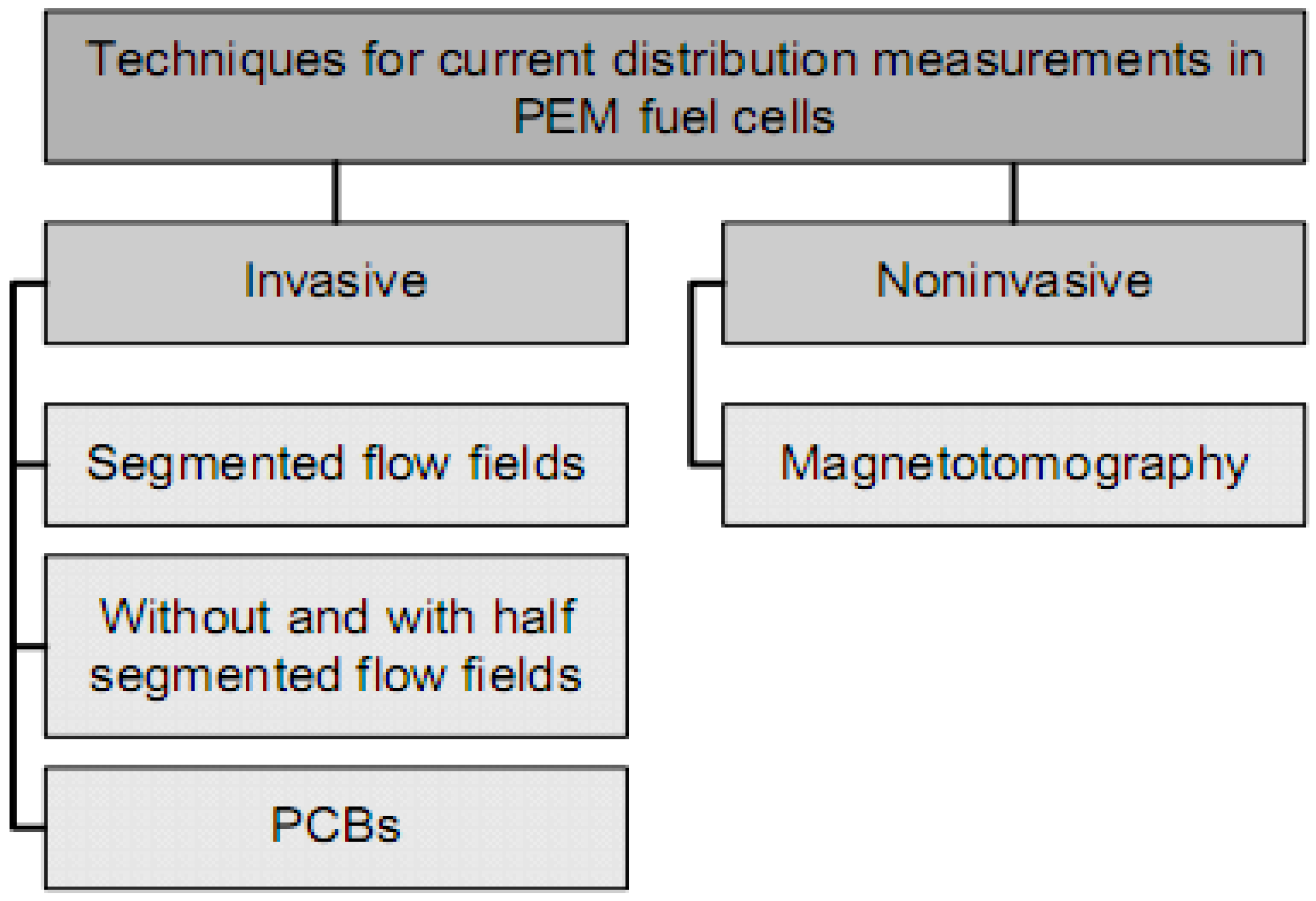
Essentially the known methods for current density distribution measurement can be divided into two main groups: non-invasive and invasive techniques (see Figure 1). Presently, the only known non-invasive method is magnetotomography [9], which requires no additional modifications on the fuel cell stack. As a rule, the measurement techniques are invasive processes, which require several modifications of the utilized fuel cell components like bipolar plates and membrane electrode assembly (MEA). The invasive techniques can be distinguished by methods using segmented and not segmented cell configurations. The measurement of local currents with resistors can be taken either outside (ex-situ) [8] or inside (in situ) [11,12] the fuel cell system. An alternative solution is to use hall sensors to determine local currents without inserting additional resistances into the system [13,14,15].

Figure 1. Overview of already realized CDD measurement techniques, cp. [16].

Figure 1. Overview of already realized CDD measurement techniques, cp. [16].

CDD measurements with segmented flow fields are sometimes taken using active procedures. The bipolar plates in PEM fuel cells balance the differences of the electric potential in the cross section, so a segmented cell configuration can control the segment voltages with the intent to measure the local currents with it. To do this, the segment voltages are regulated through a multi channel electric load to a set point. Then the local currents can be measured as given in [17,18].

Several CDD measurement systems have been developed without using segmentations. Segmentations can be avoided in systems utilizing printed circuit boards (PCB) or methods which measure local currents at the end plate [11,15]. An integration of the sensor unit inside a PCB or end plate contacts the surface of the sensing elements with adjacent not segmented bipolar plates. Thus, it is not necessary to apply an especially adapted assembly with multi channel potentiostats. The previously studied measurement methods impose quite different requirements on the manufacturing and integration of the individual parts of the measurement system.

A sensor unit, which requires no segmentation of the cell configuration, needs less effort in the development phase and can be adapted faster to other types of PEMFC. Therefore, a separately developed sensor device has an advantage which makes it possible to integrate multiple sensor plates. This multiple integration could be used to examine local currents with regard to both the length of the fuel cell stack and the dynamic behavior.

Hall sensors are quite suitable for large local currents which can be expected for a lower amount of segments. Shunt resistors are better for higher resolutions because of their small package dimensions. Another aspect is that a measurement with shunts causes less systematic error due to better long term stability. Likewise, dynamic measurements should be possible. In this way the magnetotomography is not able to measure such dynamic processes with a high spatial resolution. With an exemplary resolution of 10 × 10 measurement cells, a minimal sample time of 1s is necessary to measure physical effects in the range of diffusion constants. Based on the electric potential conditions in PEMFC the electronics should be capable to acquire the data potential-free.

3. The New CDD Measurement System

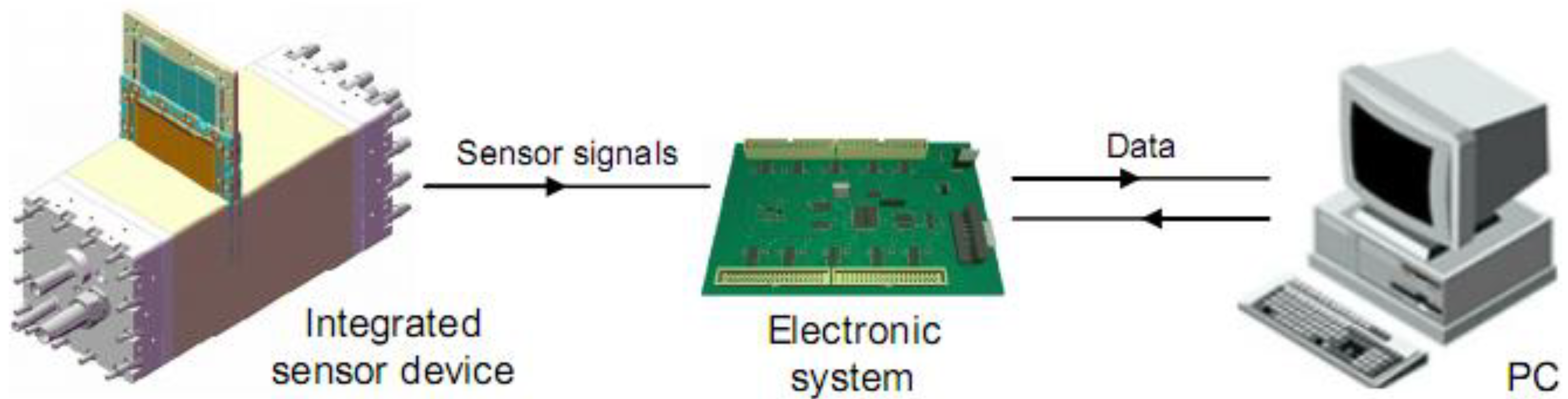
The newly developed CDD measurement system consists of three main parts: a sensor device, a data processor electronics device, and process control and visualization PC. Figure 2 shows the simplified schematic of the measurement system. A sensor device, which was positioned within the fuel cell stack, was used for data acquisition of the current density distribution. The sensor device is made up of a matrix containing 112 shunt resistors inside an epoxy resin layer with buried vias conducting local currents for coated segments through sensors to the opposite segments. The analogous sensory signals are routed to the electronics device where they are converted to digital data. Over a serial interface the digital data are sent to a superordinated measurement PC. The scaling of the raw data as well as the saving and visualizing of the computed data is performed by a specially implemented software application.

Figure 2. Schematic assembly of the measurement system.

Figure 2. Schematic assembly of the measurement system.

3.1. The Sensor Device

The sensor unit consists of a shunt matrix with 112 elements for determination of the local current densities. The active multi layer (AML^®) integration technology was used to integrate the sensor elements inside of a multi-layer printed circuit board (PCB). The sensors are low ohmic shunt resistors which are embedded in a solid epoxy resin layer. Buried vias connect the sensors with the segments outside which are in contact with the adjacent bipolar and cooling plates.

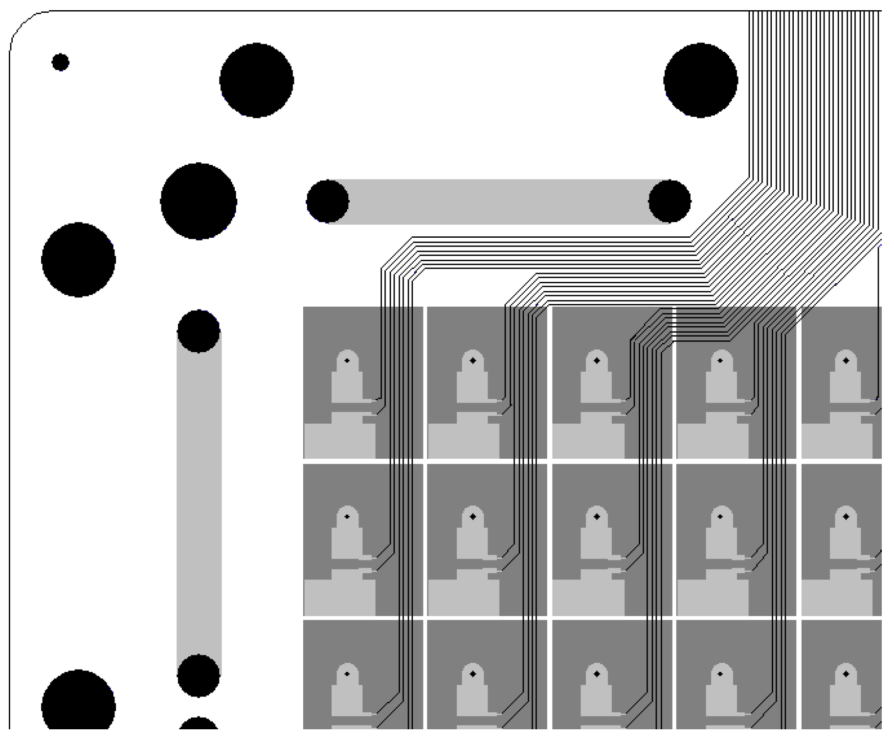
In Figure 3, the sense lines of the sensors are routed to the border of the sensor unit. A connector is located at the border and carries the sensor voltages to the converting electronics by using ribbon cables. The resolution and segmentation of the sensor device surface is adapted to the flow-field design of the chosen PEMFC system. Concerning the amount of channels it is important to take a whole number of segments for an individual flow-field direction. This is recommended to avoid measurement errors induced by measuring overlapping regions of local currents with both flow-field directions. In addition, it is useful to set the same surface area for every segment. One uniform unit of area surface size reduces the complexity in computing the values of the current densities and keeps the system intervention more balanced. The sensor elements are especially chosen for a very low temperature coefficient, slim package and long term stability. A low temperature coefficient holds the resistor value approximately constant in a typical measurement range for a PEMFC between 20 and 70 °C. The applied shunt from Isabellenhütte features a temperature coefficient that provides a weak increasing resistor value below 0.12% inside of the mentioned temperature range. In comparison with other chip resistors, it has a very slim packaging that results in a slim sensor unit.

Figure 3. Part of a sensor device layout with borings and buried vias.

Figure 3. Part of a sensor device layout with borings and buried vias.

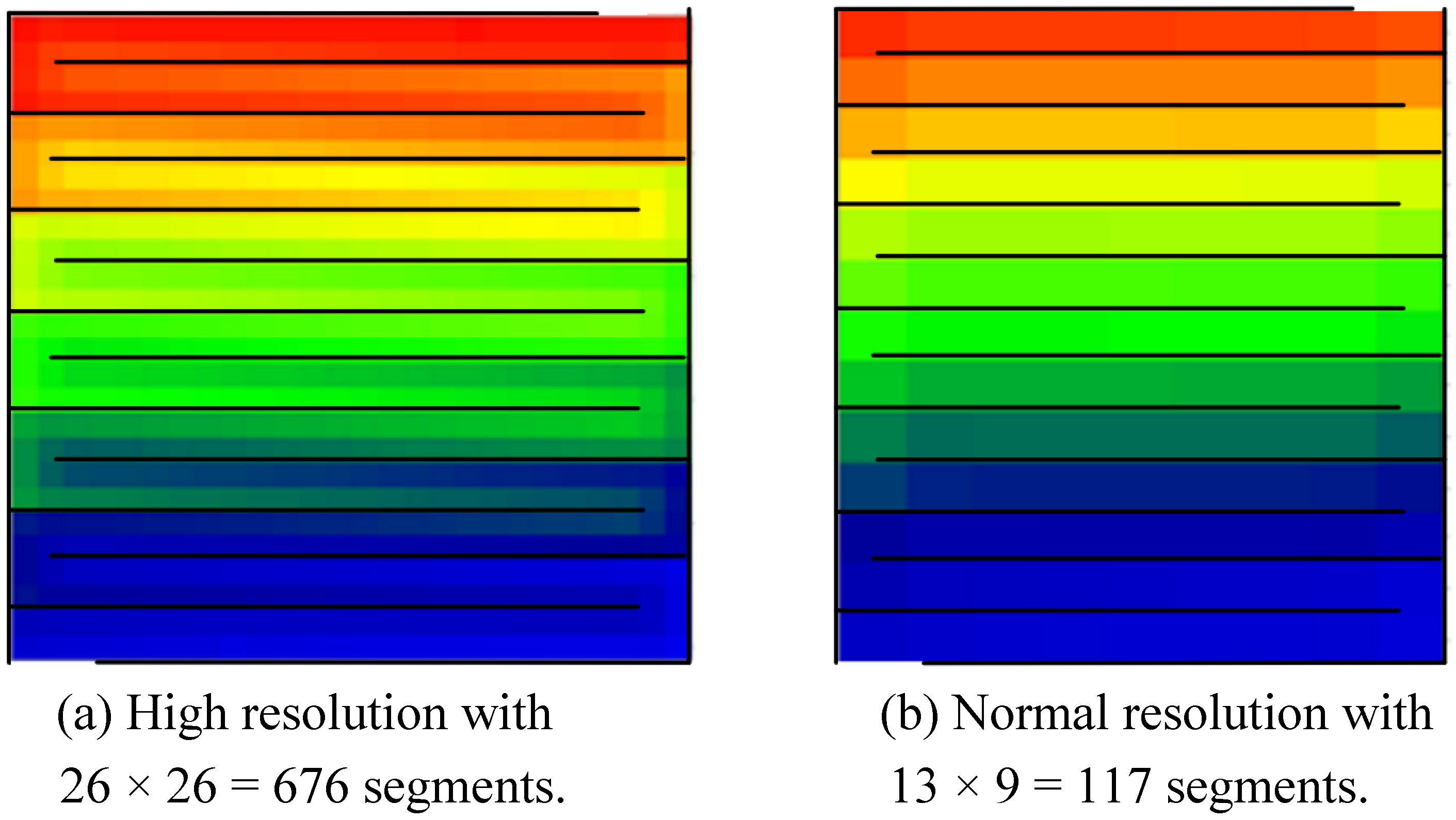
An optimal resolution for a sensor device ensures a balance between the complexity of hardware and the amount of information gained. A sensor device with high resolution, as shown in Figure 4a, has six times the amount of sensing lines and electronics for data conversion than a sensor with normal resolution (see Figure 4b). Thus, a sensor unit was designed for 8 × 14 = 112 segments. This segmentation is similar to the resolution in Figure 4b and fulfills the requirements concerning an adequate spatial resolution and reasonable complexity of electronics for data conversion.

Figure 4. Different resolutions for serpentine flow channels.

Figure 4. Different resolutions for serpentine flow channels.

3.2. Electronics for Data Conversion and Acquisition

The selected sensor elements provide a 1% tolerance of the resistor value. In this way, the data conversion of the electronics should be more precise by one degree. The accuracy of the electronic device is achieved through a high resolution 15 bit ΣΔ-Analogue-Digital-Converter (ADC). The high resolution and the good filter properties compensate for the disadvantage of the higher conversion time, because a sufficient sampling time of around 4Hz can be realized. An application with multi channel ΣΔ-ADCs eliminates the need for multiplexer handling.

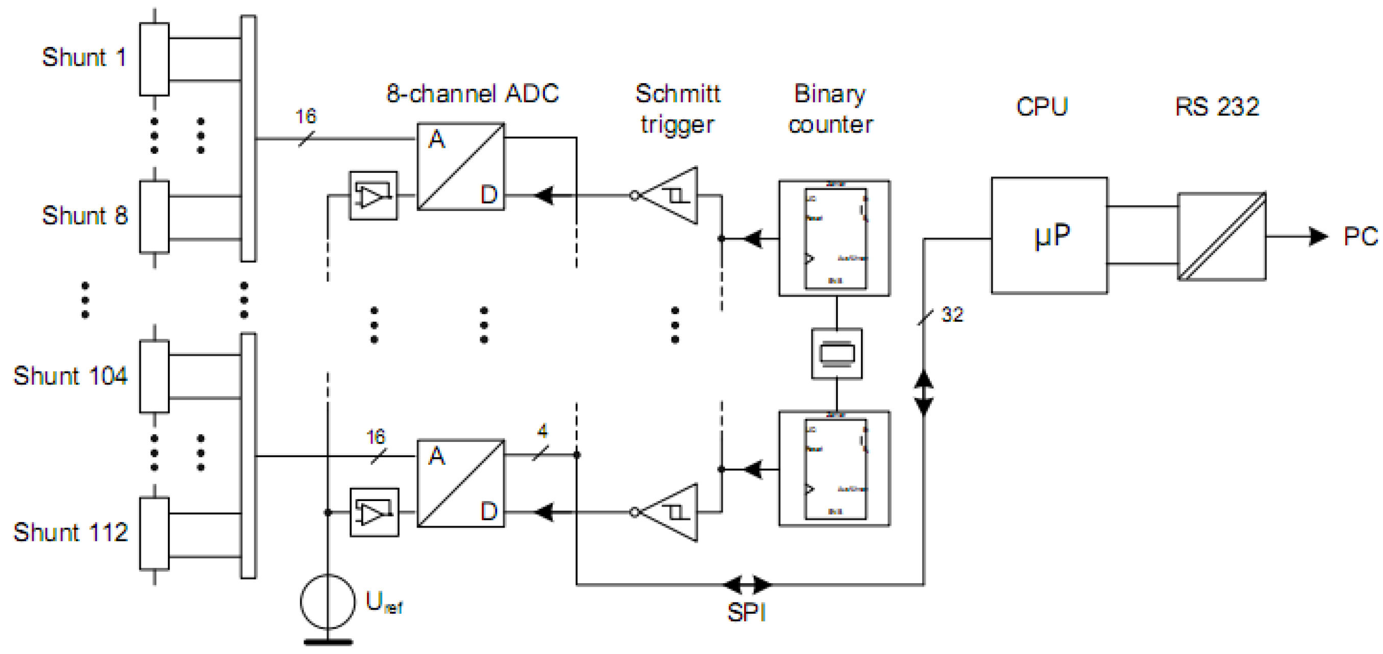
The schematic structure of the electronics in Figure 5 shows that the multi channeled ADCs are connected to the voltage reference separately, which is adapted according to the measurement range and the chosen shunt value. To shorten the conversion time or to increase the sampling rate an external oscillator, whose frequency is divided by binary counters is connected to the external oscillator inputs of the ADCs. The Schmitt triggers improve the edges of the external oscillator clock pulses. The frequency, the clock wires and the PCB layout are carefully designed to prevent signal distortion and reflections which could decrease the accuracy of the ADCs caused by the external oscillator. The ADCs are read out over a serial peripheral interface (SPI) from a microcontroller. An optical RS-232 interface is used to send the data frame to the measurement and monitoring PC.

Figure 5. Schematic of the developed electronics

Figure 5. Schematic of the developed electronics

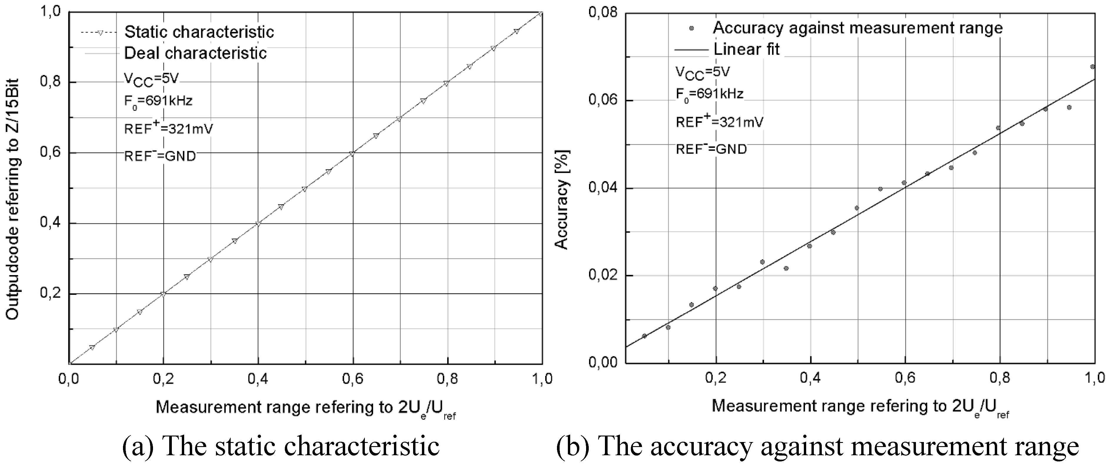
The static characteristic of the electronics in Figure 6a demonstrates an almost ideal linear characteristic that reflects a very precise output transition. Figure 6b ameliorates an analysis of the accuracy in function of the measurement range. A verification of different measurement values shows that the electronics device provides measured data with accuracy at a maximum of 0.07% in the end of the scale. The determination of accuracy in relation to the oscillator frequency revealed that the accuracy can not ensure the defined maximum of 0.1% for frequencies higher than 900 kHz. Thus, an external oscillator frequency F₀ of 691 kHz was adjusted to keep the accuracy sufficiently below 0.1%.

Figure 6. The performance characteristics of the measurement electronics.

Figure 6. The performance characteristics of the measurement electronics.

3.3. Calibration of Varying Sensors

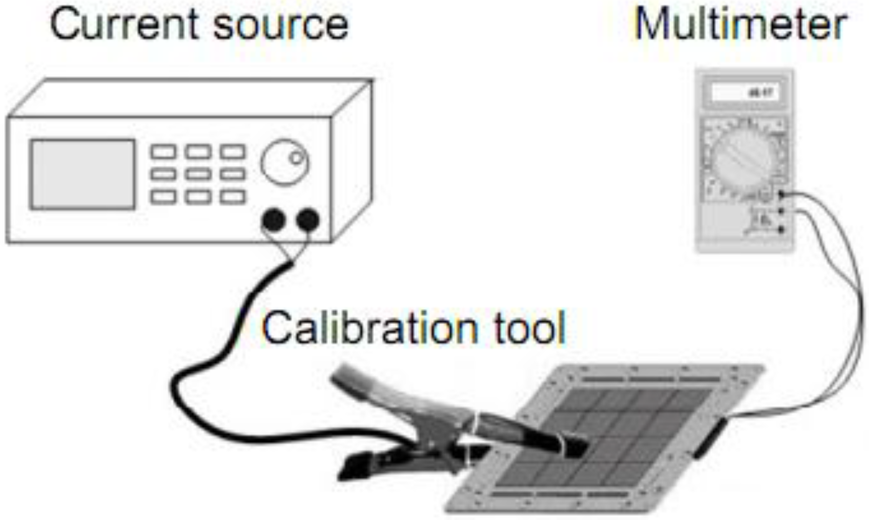
Due to the tolerance of the resistors a variation of the sensor signals may be expected in the same dimension. This creates measurement errors which can be taken into consideration by determining the real resistor values. Hence, it is possible to define correction factors to clear the induced measurement deviation. A simple method to determine the resistor values is shown in Figure 7.

Figure 7. Assembly for determination of calibration factors.

Figure 7. Assembly for determination of calibration factors.

The correctness of this arrangement depends on the accuracy class of the used instruments. The accuracy of the current source was precisely defined with a deviation of 0.06% for a current flow of 500 mA. With regard to the accuracy of the multimeter an aggregated accuracy of the arrangement can be calculated through the maximal deviation in Equation (1) and the probable deviation of the expected resistor values in Equation (2).

$$\mathrm{\Delta }{R}_{\max }={\displaystyle \sum _{i=1}^2\left|\partial \frac{R}{\partial x_i}\cdot \mathrm{\Delta }{x}_i\right|}=\left|\frac{\partial R}{\partial U}\cdot \mathrm{\Delta }U\right|+\left|\frac{\partial R}{\partial I}\cdot \mathrm{\Delta }I\right|$$

(1)

$$\mathrm{\Delta }{R}_p=\sqrt{{{\displaystyle \sum _{i=1}^2\left(\partial \frac{R}{\partial x_i}\cdot \mathrm{\Delta }{x}_i\right)}}^2}=\sqrt{{\left(\frac{\mathrm{\Delta }U}{I}\right)}^2+{\left(-\frac{U}{I^2}\cdot \mathrm{\Delta }I\right)}^2}$$

(2)

These two ways to evaluate the accuracy of this calibration method indicates a range of accuracy between 0.202% for the probable deviation and 0.209% for the maximal deviation. It should be mentioned that the probable deviation is more closely related to the real deviation and is below the maximal deviation.

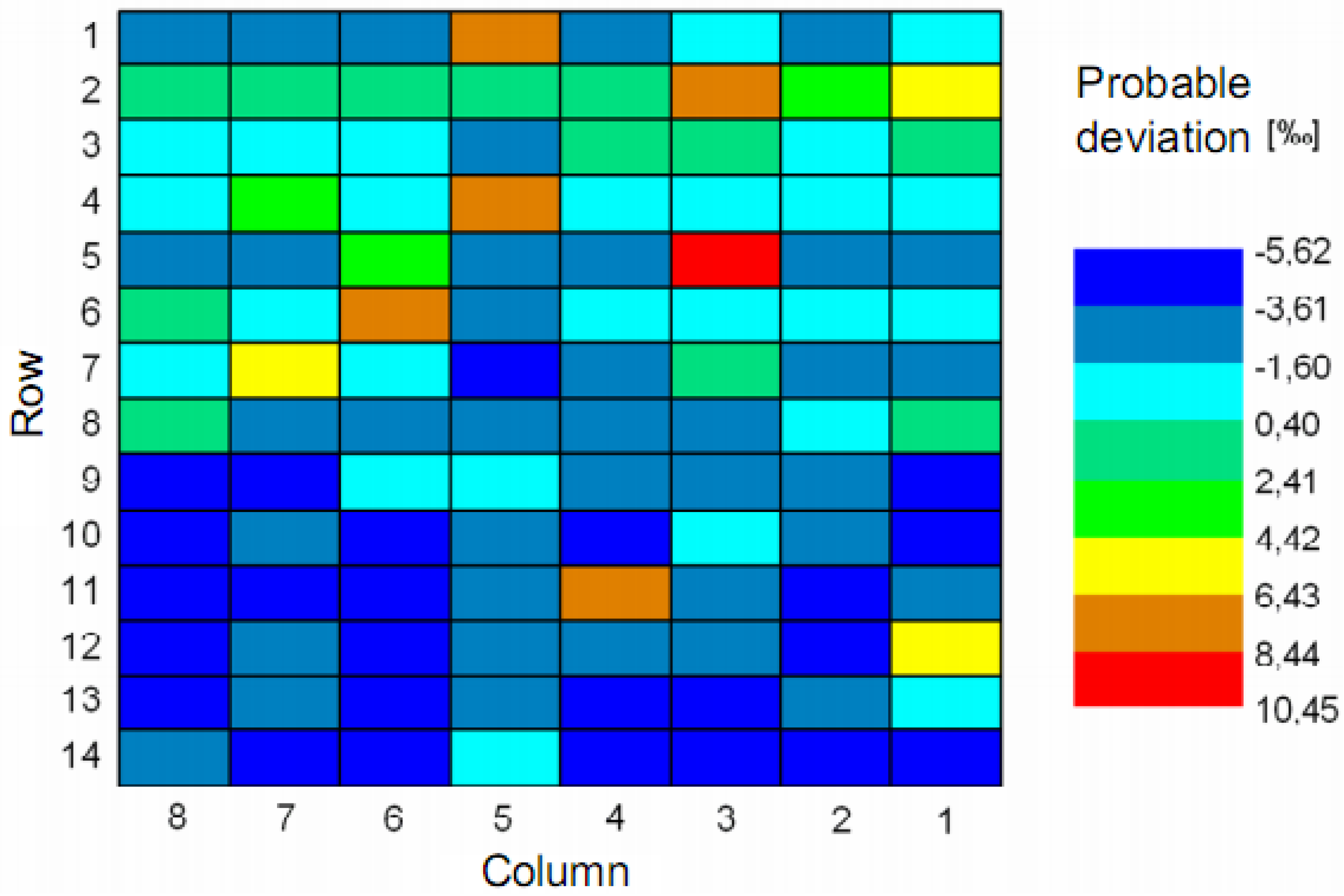
The measured resistor values are evaluated in relation to their expected values and illustrated in Figure 8. The calculated deviations are inside the tolerance range of the sensors designated by the manufacturer.

Figure 8. Probable deviation (%) of the resistors inside the sensor unit.

Figure 8. Probable deviation (%) of the resistors inside the sensor unit.

3.4. Reactions and Accuracy of the Measurement System

The mechanical fitting of the sensor unit to the fuel cell system causes differing contact resistances between the segments and the adjacent cooling and bipolar plates. This is caused by varying contact forces and certain impurities of the surfaces. The contact resistance and its deviation bring an uncertainty to the measurement through undesired lateral currents. An estimation of the dimension of the contact resistance R_c can be carried out for a contact force F_c higher than 0.1 N with Equation (3) cp. [19].

$$R_c=0.89\cdot \rho \cdot \sqrt{\frac{H}{F_c}}$$

(3)

For two different contact partners the specific electrical resistance ρ is calculated from the arithmetical average of the volume resistivities of both materials. Furthermore, the hardness of the softer material must be inserted to equation (3). The gold coating of the segments can be considered as the softer material in comparison to the carbon and graphite containing plates.

Including the constants of the used materials in Table 1 the contact resistance lies between 3.34 mΩ and 6.25 mΩ for one segment surface and the applied contact pressure of 110 N/cm². As a consequence, the contact resistance for one measurement segment makes a part between 4.4% and 8.3% in relation to the resistor value of 150 mΩ.

Table 1. Material constants of the contact partners [20].

Material	Gold	FU-4369
ρ [μΩcm]	30.8	19 000
Hardness H	HV 5.7..20	100 HR10/40

Table 1. Material constants of the contact partners [20].

Material	Gold	FU-4369
ρ [μΩcm]	30.8	19 000
Hardness H	HV 5.7..20	100 HR10/40

Probable reactions, such as lateral currents can be induced by these varying contact resistances. In addition, the sensors and differing conduction resistances inside the volume are further reasons for lateral currents. If non-segmented bipolar and sensor plates are in use higher lateral currents can appear. This fact was proven by simulations [11] as a worst-case estimation for these two types of plates and different values of measurement resistors. To find out a value for the chosen shunts a regression equation based on these simulation results was determined.

$${\widehat{i}}_{lat}[\%]=3.44468\cdot e^{-\left(\frac{R_{shunt}}{0.71351}\right)}-3.12146\cdot e^{-\left(\frac{R_{shunt}}{2.09512}\right)}+11.24236$$

(4)

Equation (4) evaluates the maximal lateral current related to the whole current with 11.4%. Wieser et. al. [14] used a magnetic loop array which consists of a segmented flow field plate to measure the current density distribution in PEMFC. An advantage of this measurement technique is that it does not have contact and measurement resistances that elevate lateral currents. Therefore, it was possible to determine lateral currents around 5% between adjacent segments. In [1] the measurement of the current density distribution was realized by carrying the local currents over external resistances to a load. For this experimental setup the maximal lateral current was specified with 10%. The lateral currents are seen as a negative reaction produced from this type of measurement technique. Hence, this influence generates an error in measurement that must be evaluated in relation to the accuracy class of the whole measurement system.

Table 2 lists the accuracies of the presented system parts that must be taken into account for the evaluation of the whole measurement system. The combined accuracies represent a class of accuracy that is normally assigned for production measurement equipment or for operational measurements. This fact is mainly caused by emerging lateral currents that have to accept using this kind of measurement principle.

Table 2. Accuracies of the measurement system parts.

Parameter	Accuracy [%]
Electronics	0.07
Tolerance of sensor	1.00
Temperature dependency of sensor	0.13
Lateral currents	11.40

Table 2. Accuracies of the measurement system parts.

Parameter	Accuracy [%]
Electronics	0.07
Tolerance of sensor	1.00
Temperature dependency of sensor	0.13
Lateral currents	11.40

4. Studies of Current Density Distributions

4.1. Experimental Setup

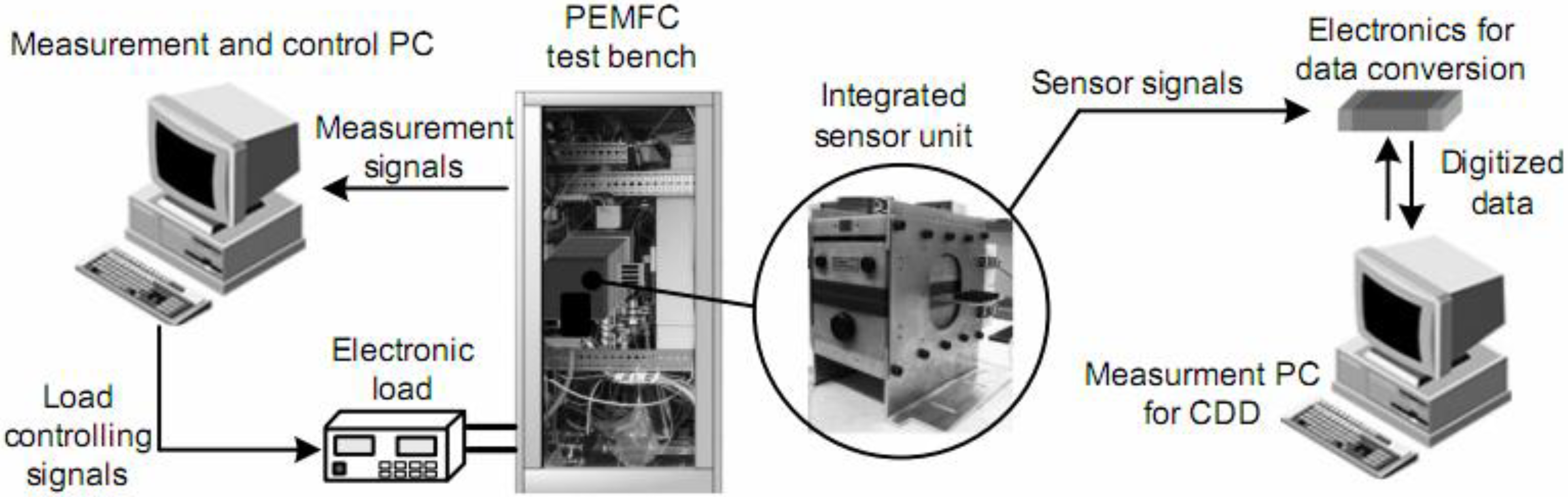
For the first experimental studies a PEMFC system with 5 cells, an active area of 200 cm² and power of 300 W was selected. The sensor device was integrated between the second and the third cell. The adjacent anode side bipolar plate contains an intermediate structure for cooling between the sensor unit and the cell. The system pressures for the reactants were in the range of 0–0.4 bar. Figure 9 illustrates the body of the PEMFC test bench consisting of a measurement PC controlling the electronic load of the independently working fuel cell system. The measurement PC stores data in periods of 10 seconds. Generally the sample time of the CDD measurement system was set to 1 second.

Figure 9. Schematic of the experimental setup.

Figure 9. Schematic of the experimental setup.

4.2. Start Up

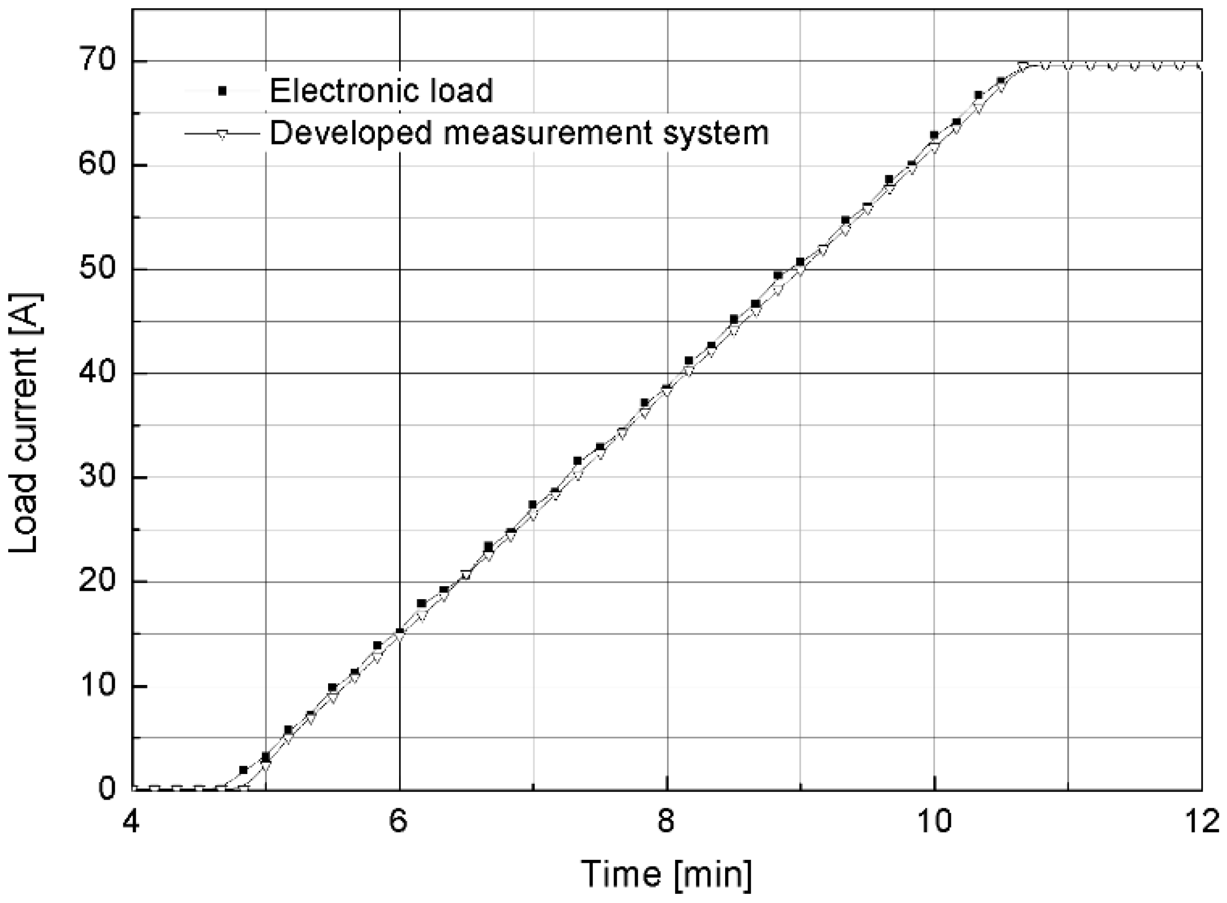
The start up of the whole fuel cell test bench was realized by a ramp-wise augmentation of the load current from 0 to 70 A with an oxygen stoichiometry ξ_air of 2.4 and a hydrogen stoichiometry ξ_H2 of 2.0. The comparison between the measurement PC and the CDD measuring device in Figure 10 illustrates close running curves. The variation between the measured curves is nearly 300mA and indicates the sufficiently good measurement accuracy of the developed system.

Figure 10. Start up phase of the PEMFC test bench.

Figure 10. Start up phase of the PEMFC test bench.

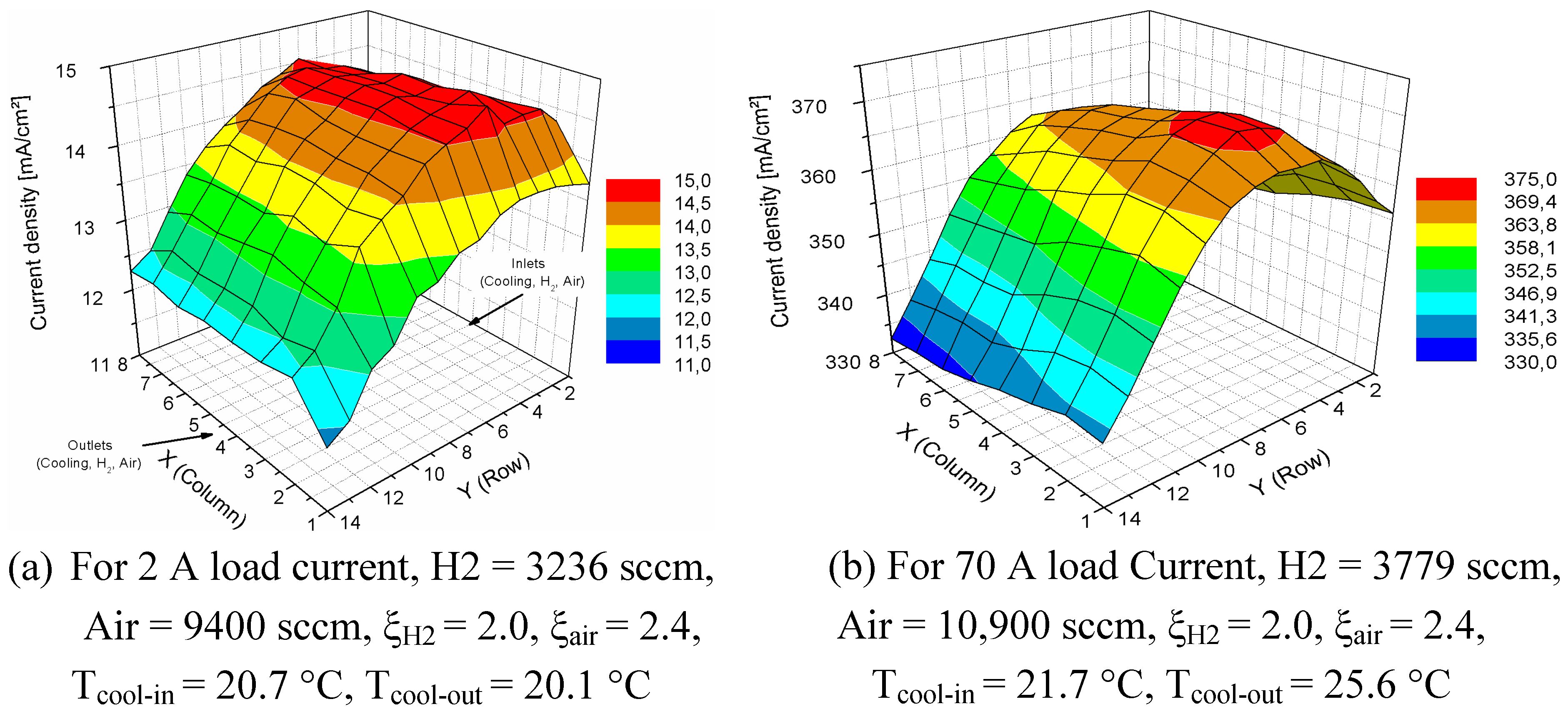
Figure 11a,b indicates that the local currents at the inlets near the first row are the highest. Due to a comparatively better humidity an improved chemical activity at the inlet supports the current production.

Figure 11a shows the current density profile at the beginning of operation. The maximal difference between the local current densities amounts to 4 mA/cm². At the end of the start up the maximal difference increases up to 39 mA/cm². The type of profile is basically preserved and depends on the humidity conditions in the membrane as well as on the flow field structure.

Figure 11. Measured current density distributions during the start up.

Figure 11. Measured current density distributions during the start up.

4.3. Warm up Phase

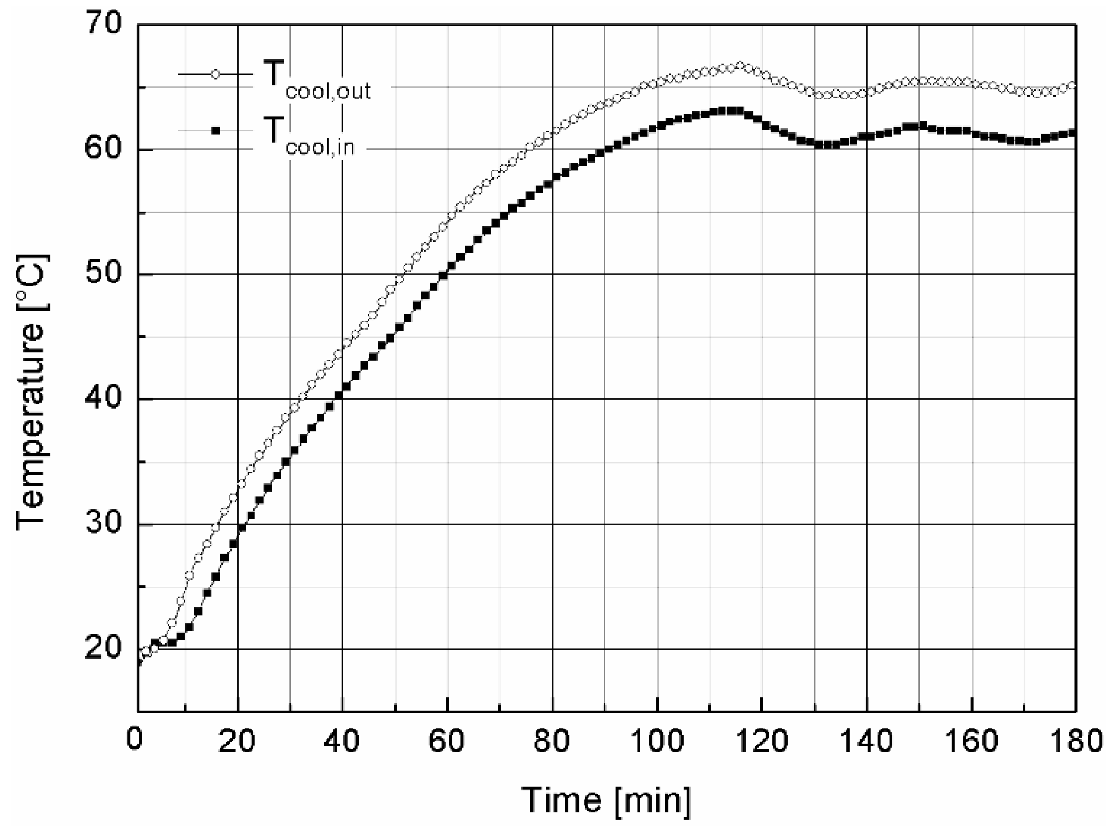
The warm up phase is necessary to reach the operating system conditions. For this purpose the fuel cell system was warmed up to 65 °C for a constant load current of 70 A. The reference variable for the temperature control is implemented through the outlet temperature of the cooling circuit. In terms of data reduction the sample time of the electronics was decreased to 5 seconds.

Figure 12. In- and outlet temperatures of the cooling circuit.

Figure 12. In- and outlet temperatures of the cooling circuit.

The curves in Figure 12 show the warm up phase from 12 to 100 minutes. After 100 minutes several overshoots are recognizable which are caused by the relatively large time constant of the water cooling circuit.

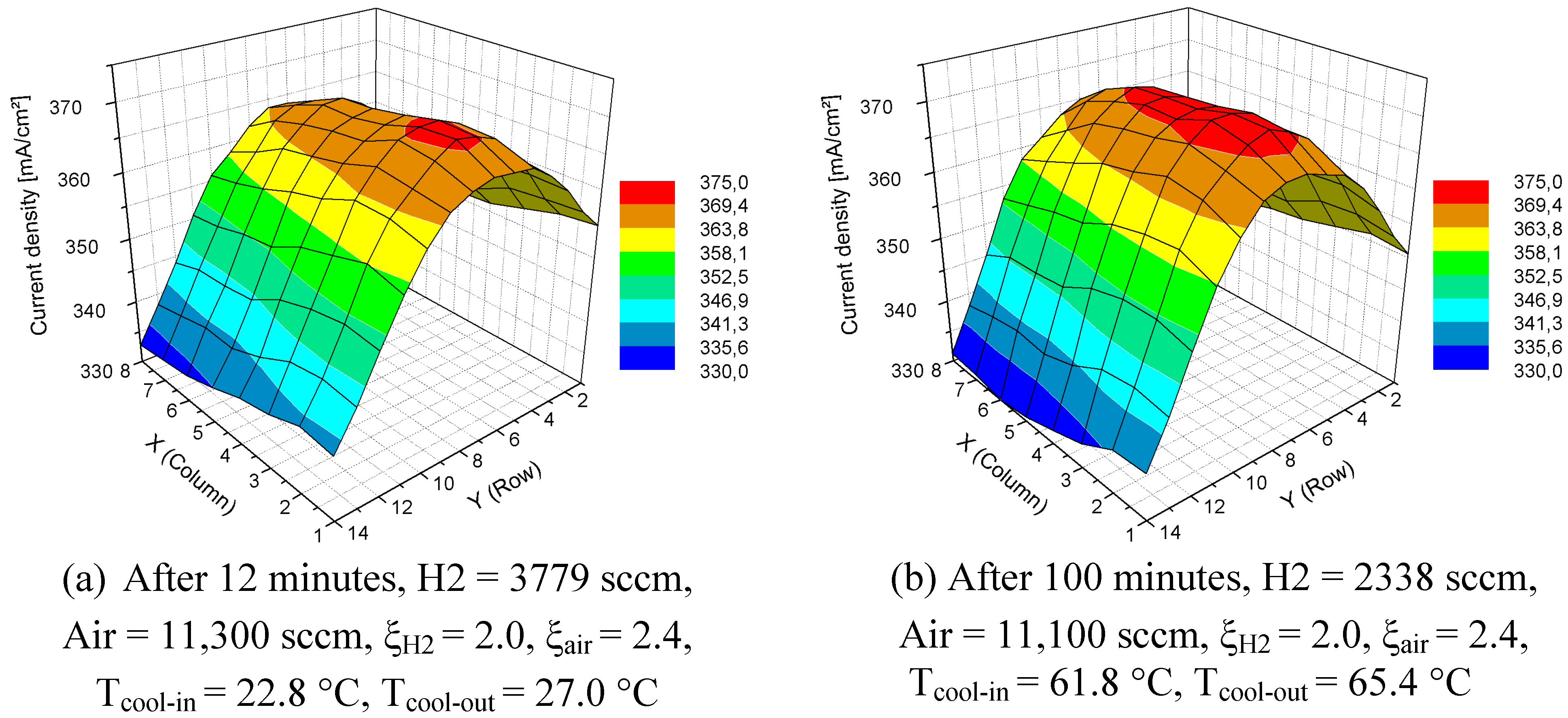
In Figure 13a, the current density profile at the beginning of the warm up has a maximal difference between the local current densities of 38 mA/cm². After 100 minutes of warm up, Figure 13b shows minimal changes in this profile. The maximal difference has increased slightly up to 42 mA/cm² and the area of maximal current production has shifted a bit to the middle of the flow path. Because the changes in the current density profile during the warm up are small, the temperature influence could be neglected in this phase.

Figure 13. Measured current density distributions during the warm up phase.

Figure 13. Measured current density distributions during the warm up phase.

4.4. Operating Area

After the warm up phase is completed, the load current was once again ramp-wise elevated from 70 up to 100 A. A load current of 100 A represents the operating area of this fuel cell system. The contour of the current density profile shown in Figure 14 is similar to the already represented plots but with a maximal difference of 60 mA/cm².

Figure 14. Current density distribution for 100 A load current. H2 = 3254 sccm, Air = 15,800 sccm, ξ_H2 = 2.0, ξ_air = 2.4, T_cool-in = 60.4 °C, T_cool-out = 66.7 °C

Figure 14. Current density distribution for 100 A load current. H2 = 3254 sccm, Air = 15,800 sccm, ξ_H2 = 2.0, ξ_air = 2.4, T_cool-in = 60.4 °C, T_cool-out = 66.7 °C

5. Conclusions

This paper describes the development and functionality of a newly developed measurement system for current density distribution mapping with regard to operational modes in PEMFC. The sensor device is developed within a multi layer technology that allows for the integration of shunt resistors inside a printed circuit board. The sensor unit is fitted to the geometry of the flow field channels of the fuel cell system being used. Therefore, usual CAD software enables a faster adaptation to different flow field and stack geometries.

To calibrate the measurement deviation, the tolerances of the integrated shunts can be considered with the method presented in this paper. The investigated accuracies and reactions of the system indicate that lateral currents can affect a measurement error by as much as 10%. Thus, the intended system is evaluated as equipment to measure profiles of current production because of the resulting accuracy class. In this respect the developed system is well suited to operational measurements.

The results of the provided experiments show the significance of the measured data in terms of different working areas of a PEMFC. The measured current density distributions during the warm up phase show a negligible influence of the temperature to the current density profile of the selected fuel cell system. At different operating points the maximum of the local current production is close to the inlet of atmospheric oxygen. Nevertheless the load current induces different grades of inhomogeneity. The operational area of the fuel cell system amounts to a maximal difference between the local current densities of 59 mA/cm². In relation to the maximum of 531 mA/cm², a percent difference of 11.2% reveals the optimization potential for a homogenous current density distribution profile.