Short-Term Load Forecasting for Electric Power Systems Using the PSO-SVR and FCM Clustering Techniques

Abstract

This paper presents a new combined method for the short-term load forecasting of electric power systems based on the Fuzzy c-means (FCM) clustering, particle swarm optimization (PSO) and support vector regression (SVR) techniques. The training samples used in this method are of the same data type as the learning samples in the forecasting process and selected by a fuzzy clustering technique according to the degree of similarity of the input samples considering the periodic characteristics of the load. PSO is applied to optimize the model parameters. The complicated nonlinear relationships between the factors influencing the load and the load forecasting can be regressed using the SVR. The practical load data from a city in Chongqing was used to illustrate the proposed method, and the results indicate that the proposed method can obtain higher accuracy compared with the traditional method, and is effective for forecasting the short-term load of power systems.

1. Introduction

Short-term load forecasting (STLF) aims at predicting the system load over a short time period like a day or a week, and plays an important role in power system operation. Many load forecasting approaches have been reported in the last decade, such as conventional smoothing technique, regression method, statistical analysis, time series analysis, autoregressive moving average model, and expert system [1,2]. Although these techniques and models are reliable and useful, they are not suitable for analyzing unusual weather conditions and varied holiday activities, which usually result in a daily load with highly non-linear characteristics.

Load forecasting for any given day is a difficult task, because it depends not only on the load of the previous days, but also on that on the same day in the previous weeks and even the previous years [3]. Furthermore, it is difficult to model the relationship between the load and the mentioned external factors influencing the load demand, such as weather variations, holiday activities, etc. These are the major factors making the modeling process more complicated. Because the model parameters are decided according to the historical data, some errors may be introduced [4].

The time series methods treat the load pattern as a time series signal with known period, and offer a rough prediction of the load for the given season. The techniques used in time series methods are as follows [5,6]: (a) Kalman Filter method; (b) Box Jenkins method; (c) Regression processes; (d) Spectral expansion technique. The spectral expansion technique utilizes the Fourier series. Generally, these techniques use a large number of complex relationships and require long computation times.

An intelligent system exhibits intelligence in capturing and processing information, and employs artificial intelligence techniques to fulfill some or all of its computational requirements. Artificial Neural Networks (ANNs) are capable of performing non-linear modeling and adaptation. In addition, they do not require a functional relationship between load and weather variables in advance. An expert system has the ability to act as a knowledge expert, therefore the load-forecast model can be built using the knowledge about the load-forecast domain provided by an expert in the field [7,8,9].

Recently methods load forecasting based on the load similarity were reported, which forecast the load curve by using the load information of the days with weather conditions similar to the objective day. In these methods several similar days are selected to improve the accuracy of load forecasting, which can not only deal with the non-linear relationship of the loads, but also the influence caused by weekends or special days. However the weights of different influencing factor cannot reflect the actual degree of influence due to the lack of adequate cognition of these factors.

In order to solve the problems mentioned above, this paper presents a novel preprocessing procedure based on the PSO-SVR and the FCM clustering techniques, which can improve the precision of daily load forecasting. Practical load data from a city in Chongqing, China, was used to demonstrate the proposed techniques, and the results indicate that the proposed method is effective for forecasting the short-term power system load.

The remaining parts of the paper are arranged as follows: Section 2 introduces the support vector regression based on PSO. Section 3 describes the short-term load forecasting process using the PSO-SVR and FCM clustering techniques, and an analysis of a practical case study follows in Section 4. Finally the conclusions will come at Section 5.

2. Support Vector Regression Base on PSO

Particle swarm optimization (PSO) was introduced by Eberhart and Kennedy in 1995 [10]. A PSO has two primary operators: a velocity update operator and a position update operator. During the convergence process, each particle is accelerated toward the particles with previous best position and the global best position. A new velocity for each particle is calculated in an iteration based on its current velocity and the distances from its previous best position and the global best position. The new velocity is then used to calculate the next position of the particle in the search space. This process is repeated until a pre-specified minimum error is met. The updated velocity and position are given by:

$$\{\begin{array}{l}{v}_{id}^{k+1}=w\times v_{id}^k+c_1\times r_1\times (p_{id}-x_{id}^k)+c_2\times r_2\times (p_{gd}-x_{id}^k)\\ x_{id}^{k+1}=v_{id}^{k+1}+x_{id}^k\end{array}$$

(1)

Support vector regression (SVR) [11] is a regression method based on the SVM method. Different from SVM, SVR tries to find a hyper-plane which can accurately predict the distribution of information, but not the plane on which to classify the data. However, the prerequisite for SVR to achieve the better results is to find three appropriate parameters: the kernel function K, the balance factor C and the insensitive loss function ε, which are critical for achieving high accuracy and generalization of the regression model.

For a training sample set:

$$T={\{(x_i,y_i)\}}_{i=1}^l$$

x_i ∈ R^m is the input vector, y_i ∈ R is the corresponding objective output and l is the number of training samples.

Using a nonlinear mapping $\varphi (x)$ R^m → R^M, the SVR maps a low dimensional input space to a high dimensional feature space, then it regresses linearly in a high dimensional feature space, which can demonstrate the influence of nonlinear regression in original input space. The general function of a decision linear regression is:

$$f(x)=(w\cdot \varphi (x))+b$$

(2)

where w is a weight vector, and b is a threshold value. The parameters of the optimum regression in Equation (2) are solved using (3) to minimize the structural risk R:

$$\min R=\frac{1}{2}{\Vert w\Vert }^2+C{R}_{emp}$$

(3)

where:

$$R_{emp}=\frac{1}{l}{\displaystyle \sum _{i=1}^l(L_e(x_i,y_i-f(x_i)))}$$

(4)

$$L_e(x,y-f(x))=\max \{0,\left|y-f(x)\right|-\epsilon \}$$

(5)

The item ||w||²/2 in (3) is the expressing ability of the complexity of the decision function; the item R_emp is the training error, and C is the balance factor which indicates the degree of matching of the two parts above. Experience risk R_emp is measured by the loss function, which usually adopts the insensitive loss function $L_e(x,y-f(x))$.

By introducing the slack variables ${\xi }_i$ and ${\xi }_i^{\ast }$ ($i=1,2,\mathrm{...},l$), Equation (3) can be rewritten as:

$$\min \frac{1}{2}{\Vert w\Vert }^2+\frac{C}{l}{\displaystyle \sum _{i=1}^l({\xi }_i+{\xi }_i^{\ast })}$$

(6)

$$\text{St}:\{\begin{array}{c}(w\cdot \varphi (x_i))+b-y_i\le \epsilon +\xi \\ y_i-(w\cdot \varphi (x_i))-b\le \epsilon +\xi \\ {\epsilon }_i,{\epsilon }_i^{\ast }\ge 0(i=1,2,\mathrm{...},l)\end{array}$$

Equation (6) is called the primitive problem of SVR. The primitive problem is actually a problem with linear constraints.

Introducing the Lagrange multipliers to the Lagrange function, the partial derivative of the Lagrange function with respect to $w$, $b$, ${\xi }_i$, ${\xi }_i^{\ast }$ can be obtained, and its dual problem is given by:

$$\min \frac{1}{2}{\displaystyle \sum _{i=1}^l({\alpha }_i^{\ast }-{\alpha }_i)}({\alpha }_{\text{j}}^{\ast }-{\alpha }_j)K(x_i,x_j)+\epsilon {\displaystyle \sum _{i=1}^l({\alpha }_i^{\ast }+{\alpha }_i)}-{\displaystyle \sum _{i=1}^l{y}_i({\alpha }_i^{\ast }-{\alpha }_i)}$$

(7)

$$\text{St}:\{\begin{array}{c}{\displaystyle \sum _{i=1}^l({\alpha }_i^{\ast }-{\alpha }_i)}=0\\ 0\le {\alpha }_i，{\alpha }_i^{\ast }\le \frac{C}{l}(i=1,2,\mathrm{...},l)\end{array}$$

$$\text{St}:\{\begin{array}{c}\overline{b}=y_j-{\displaystyle \sum _{i=1}^l({\overline{\alpha }}_i^{\ast }-{\overline{\alpha }}_i)(x_i,x_j)}+\epsilon \\ if {\overline{\alpha }}_j\in (0,\frac{C}{l})\\ \overline{b}=y_j-{\displaystyle \sum _{i=1}^l({\overline{\alpha }}_i^{\ast }-{\overline{\alpha }}_i)(x_i,x_j)}-\epsilon \\ f {\overline{\alpha }}_j^{\ast }\in (0,\frac{C}{l})\end{array}$$

where $K(x_i,x_j)=(\varphi (x_i)\cdot \varphi (x_j))$ is a kernel function. The kernel function is used to obtain the decision-making regressive equation without knowing the definite form of nonlinear mapping $\varphi (x)$ from the low dimensional input space to high dimensional feature space.

Assuming that $\overline{\alpha }={({\overline{\alpha }}_1,{\overline{\alpha }}_1^{\ast },\mathrm{...},{\overline{\alpha }}_l,{\overline{\alpha }}_l^{\ast })}^T$ is the solution of dual problem, there is at least a zero in a pair of $({\overline{\alpha }}_i,{\overline{\alpha }}_i^{\ast })$ according to the sparse characteristic of the SVR.

Decision function is only determined by support vectors and has nothing to do with nonsupport vectors. Decision regression function (2) can be written as:

$$f(x)={\displaystyle \sum _{i=1}^l({\overline{\alpha }}_i^{\ast }-{\overline{\alpha }}_i)K(x_i,x)}+\overline{b}$$

(8)

3. Short-Term Load Forecasting Using the PSO-SVR and FCM Clustering Technique

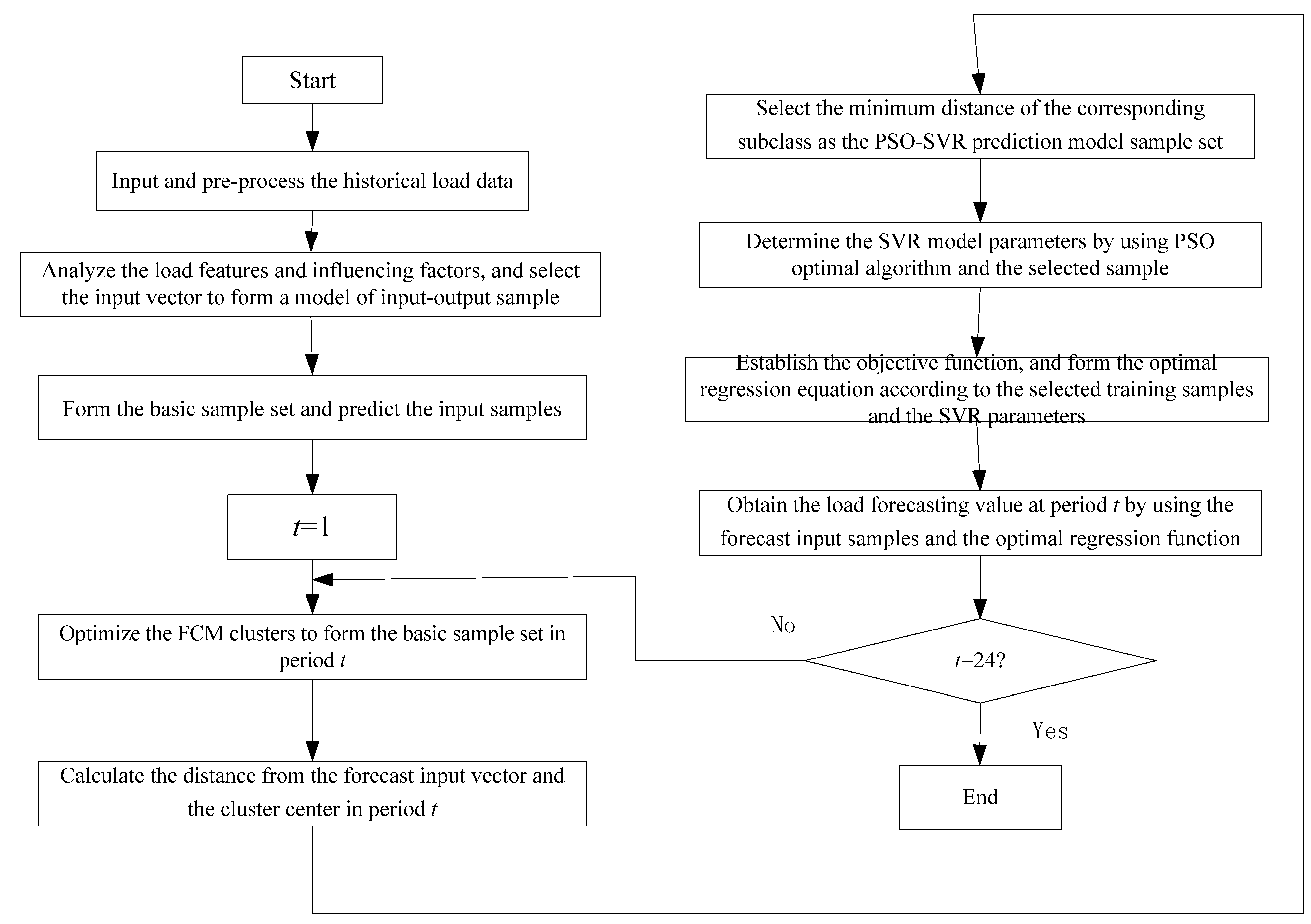
This section presents the optimum FCM clustering analysis and a new short-term load forecasting method using the PSO-SVR and FCM clustering technique.

Fuzzy c-means (FCM) is a clustering method which allows a large number of data to be classified into two or more clusters. This method (developed by Dunn in 1973 [12] and improved by Bezdek in 1981 [13]) is widely used in pattern recognition. The FCM is formulated as a model of minimizing the following objective function:

$$J_m={\displaystyle \sum _i^N{\displaystyle \sum _j^C{u}_{ij}^m{\Vert x_i-c_j\Vert }^2,1\le }}m<\infty$$

(9)

where m is any real number greater than 1, u_ij is the degree of membership of x_i belonging to cluster j, x_i is the ith of d-dimensional measured data, c_j is a d-dimension center of the cluster, and ||*|| is any norm expressing the similarity between any measured data and the center.

Fuzzy partitioning is carried out through an iterative optimization of the objective function shown above, with the updates of membership u_ij and the cluster centers c_j by:

$$u_{ij}=\frac{1}{{\displaystyle \sum _{k=1}^C{\left[\frac{\Vert x_i-c_j\Vert }{\Vert x_i-c_k\Vert }\right]}^{\frac{2}{m-1}}}}$$

(10)

$$c_j=\frac{{\displaystyle \sum _{i=1}^N{u}_{ij}^m\cdot x_i}}{{\displaystyle \sum _{i=1}^N{u}_{ij}^m}}$$

(11)

The iteration is stopped when ${\max }_{ij}\left\{\left|u_{ij}^{(k+1)}-u_{ij}^{(k)}\right|\right\}<\epsilon$, where ε is a pre-specified error criterion and k is the iteration step. This procedure converges to a local minimum or a saddle point of J_m.

The main idea for the short-term load forecasting is as follows: (1) Use the FCM clustering algorithm to obtain the optimum load pattern classification samples considering the change rules of the historical daily load in a power system. (2) Use the pattern recognition method to extract the optimal training samples. (3) Construct the load forecasting model using the PSO-SVR regression algorithm. This method can reduce the number of training samples and improve the prediction accuracy of support vector machines.

The following are the details for this method:

(1)

Pre-process the historical load data and normalize the basic data. A basic sample for each predicted time can be obtained based on the input-output load data, and the forecasting input sample $x_t(t=1,2,\cdots ,N)$ is formed.

(2)

Set the kernel function and model parameters, and select the weight of the FCM cluster analysis, here $m=1.3$, the largest possible number of clusters $c_{\max }=\sqrt{n}$, where $n$ is the load sample number of the dataset used in clustering analysis, then set the pre-specified iterative convergence error of FCM clustering algorithm, here $\epsilon ={10}^{-6}$. The basic sample set for each predict time in the objective day is analyzed using optimal FCM cluster method, then the classified information of the basic sample set with the best clusters number can be collected. The distance between the forecast time period of the input samples $x_t$ is calculated, and the minimum distance corresponding to the sub-class as the PSO-SVR forecasting methods sample set will be set. By using the sample set at each forecasting time and the selected clustering parameters, the PSO-SVR load forecasting model is constructed, and the parameters for support vector machine regression algorithm are obtained. The objective function as Equation (7) can be formed and solved. Finally, by substituting the optimal solution of SVR model ${\alpha }_i$ and $b$ to Equation (8), the optimal regression function at each time period can be 0.

(3)

Use the forecast input samples and the optimal regression function at each time period to predict the load in the future.

The detail of the load forecasting process using the PSO-SVR and FCM clustering techniques is shown in Figure 1.

Figure 1. Flow chart of the load forecasting process.

Figure 1. Flow chart of the load forecasting process.

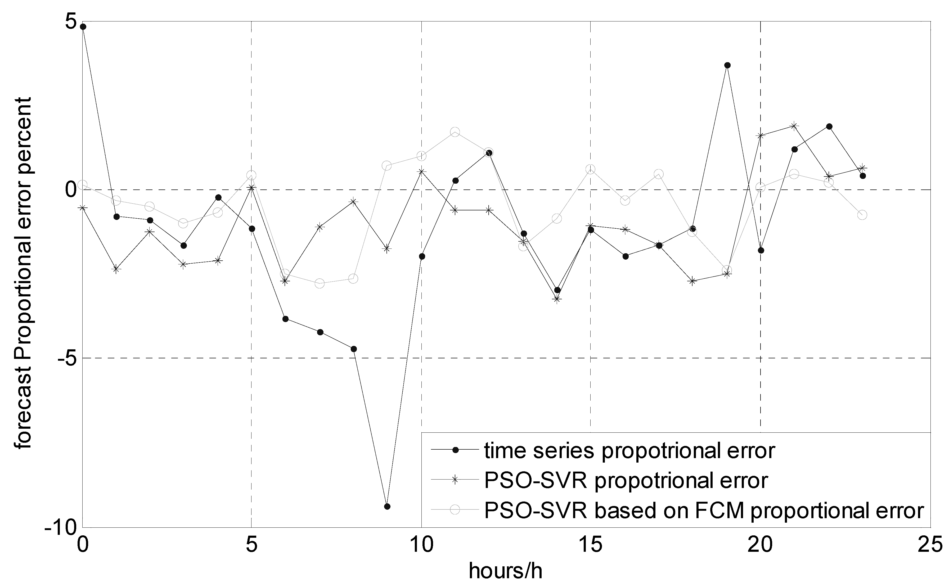
4. Simulation Results and Discussion

In order to verify the feasibility of the proposed method, a case study on the load forecasting from a city in Chongqing, China, was used. The traditional methods are first used to forecast the load, and the method in this paper is also used to forecast the short-term load, and comparisons were made to analyze the characteristics of the different methods.

The historical load data is shown in Table 1. Firstly the time series method is used to forecast the short-term load, and Table 2 shows the load forecasting results using the time series method. It can be concluded that the maximum forecasting error is 9.362%, which is a little large for practical engineering. The average error of the time series method is 1.136%.

Table 1. Historical load data.

	Month	1	2	3	4	5	6	7	8	9	10
Time(hour)
0:00		2269.5	2072.4	2082.5	2064.1	2165.3	2292.4	2308.6	2331.8	2212.9	2224.0
1:00		2013.6	1863.2	1781.9	1887.6	1967.8	2057.7	2112.1	2055.1	1985.6	1955.5
2:00		1782.3	1626.1	1724.3	1740.2	1814.3	1873.3	1889.5	1867.7	1893.8	1841.6
3:00		1684.5	1624.9	1659.0	1696.4	1721.3	1831.4	1802.3	1817.6	1822.2	1789.5
4:00		1692.4	1553.1	1611.8	1643.2	1697.8	1798.5	1793.7	1752.6	1782.9	1744.8
5:00		1622.9	1556.2	1537.4	1622.3	1713.7	1783.4	1736.5	1732.6	1747.1	1742.0
6:00		1655.7	1560.8	1577.7	1663.0	1734.9	1789.0	1786.4	1748.5	1800.3	1766.5
7:00		1704.2	1657.0	1677.7	1890.7	1974.4	2025.4	1872.1	1801.6	2009.5	1972.0
8:00		1809.8	1786.6	1792.7	1965.0	2097.7	2108.5	1955.6	1901.7	2103.5	2112.1
9:00		2043.4	2064.6	2205.2	2505.8	2658.1	2677.7	2410.3	2317.5	2593.7	2642.6
10:00		2034.7	2204.4	2369.0	2697.6	2807.4	2819.2	2604.6	2432.2	2752.4	2693.4
11:00		2168.4	2343.4	2483.1	2842.0	2955.4	2899.9	2776.4	2608.8	2880.5	2621.4
12:00		2320.7	2477.4	2553.9	2846.0	2920.5	2838.3	2781.3	2650.2	2818.8	2601.8
13:00		2130.4	2194.0	2322.9	2662.7	2832.6	2625.7	2567.6	2382.1	2551.3	2400.1
14:00		2093.3	2245.7	2408.2	2798.5	2869.8	2696.4	2619.7	2400.3	2679.1	2519.3
15:00		2119.0	2294.2	2428.9	2832.2	2764.5	2696.8	2649.7	2430.8	2649.4	2540.6
16:00		2131.2	2245.3	2454.2	2794.8	2733.3	2665.3	2666.2	2407.8	2621.6	2517.8
17:00		2213.7	2342.3	2509.8	2845.3	2799.3	2747.6	2729.0	2510.9	2698.5	2599.4
18:00		2372.5	2555.3	2707.7	2896.0	2905.7	2824.4	2820.4	2671.1	2774.4	2668.6
19:00		2584.2	2752.3	2853.2	3004.5	3122.8	3118.5	2963.1	2950.9	3016.5	2891.2
20:00		2540.3	2695.2	2859.4	2934.7	3096.8	3109.5	2014.3	3031.7	2983.2	2878.0
21:00		2569.6	2643.4	2834.3	2944.7	3083.0	3130.6	3001.0	2979.5	2982.2	2900.1
22:00		2419.4	2543.0	2602.2	2708.9	2873.8	2893.5	2817.6	2754.7	2822.2	2731.6
23:00		2199.2	2222.8	2262.1	2394.0	2558.9	2609.0	2509.3	2440.0	2458.6	2411.7

Table 1. Historical load data.

	Month	1	2	3	4	5	6	7	8	9	10
Time(hour)
0:00		2269.5	2072.4	2082.5	2064.1	2165.3	2292.4	2308.6	2331.8	2212.9	2224.0
1:00		2013.6	1863.2	1781.9	1887.6	1967.8	2057.7	2112.1	2055.1	1985.6	1955.5
2:00		1782.3	1626.1	1724.3	1740.2	1814.3	1873.3	1889.5	1867.7	1893.8	1841.6
3:00		1684.5	1624.9	1659.0	1696.4	1721.3	1831.4	1802.3	1817.6	1822.2	1789.5
4:00		1692.4	1553.1	1611.8	1643.2	1697.8	1798.5	1793.7	1752.6	1782.9	1744.8
5:00		1622.9	1556.2	1537.4	1622.3	1713.7	1783.4	1736.5	1732.6	1747.1	1742.0
6:00		1655.7	1560.8	1577.7	1663.0	1734.9	1789.0	1786.4	1748.5	1800.3	1766.5
7:00		1704.2	1657.0	1677.7	1890.7	1974.4	2025.4	1872.1	1801.6	2009.5	1972.0
8:00		1809.8	1786.6	1792.7	1965.0	2097.7	2108.5	1955.6	1901.7	2103.5	2112.1
9:00		2043.4	2064.6	2205.2	2505.8	2658.1	2677.7	2410.3	2317.5	2593.7	2642.6
10:00		2034.7	2204.4	2369.0	2697.6	2807.4	2819.2	2604.6	2432.2	2752.4	2693.4
11:00		2168.4	2343.4	2483.1	2842.0	2955.4	2899.9	2776.4	2608.8	2880.5	2621.4
12:00		2320.7	2477.4	2553.9	2846.0	2920.5	2838.3	2781.3	2650.2	2818.8	2601.8
13:00		2130.4	2194.0	2322.9	2662.7	2832.6	2625.7	2567.6	2382.1	2551.3	2400.1
14:00		2093.3	2245.7	2408.2	2798.5	2869.8	2696.4	2619.7	2400.3	2679.1	2519.3
15:00		2119.0	2294.2	2428.9	2832.2	2764.5	2696.8	2649.7	2430.8	2649.4	2540.6
16:00		2131.2	2245.3	2454.2	2794.8	2733.3	2665.3	2666.2	2407.8	2621.6	2517.8
17:00		2213.7	2342.3	2509.8	2845.3	2799.3	2747.6	2729.0	2510.9	2698.5	2599.4
18:00		2372.5	2555.3	2707.7	2896.0	2905.7	2824.4	2820.4	2671.1	2774.4	2668.6
19:00		2584.2	2752.3	2853.2	3004.5	3122.8	3118.5	2963.1	2950.9	3016.5	2891.2
20:00		2540.3	2695.2	2859.4	2934.7	3096.8	3109.5	2014.3	3031.7	2983.2	2878.0
21:00		2569.6	2643.4	2834.3	2944.7	3083.0	3130.6	3001.0	2979.5	2982.2	2900.1
22:00		2419.4	2543.0	2602.2	2708.9	2873.8	2893.5	2817.6	2754.7	2822.2	2731.6
23:00		2199.2	2222.8	2262.1	2394.0	2558.9	2609.0	2509.3	2440.0	2458.6	2411.7

Table 2. Load forecasting using the time series method.

Time (hour)	Actual Load (MW)	Forecasting Load (MW)	Forecasting Error (%)	Time (hour)	Actual Load (MW)	Forecasting Load (MW)	Forecasting Error (%)
0:00	2096.0	2202.343	4.829	12:00	2651.6	2680.889	1.094
1:00	1983.9	1968.010	−0.807	13:00	2498.6	2466.940	−1.283
2:00	1821.6	1805.310	−0.902	14:00	2608.4	2533.030	−2.975
3:00	1773.4	1744.910	−1.633	15:00	2570.5	2540.610	−1.176
4:00	1710.7	1707.080	−0.212	16:00	2573.2	2523.750	−1.959
5:00	1698.6	1679.410	−1.143	17:00	2642.1	2599.580	−1.636
6:00	1773.4	1708.286	−3.810	18:00	2751.2	2719.609	−1.161
7:00	1936.5	1858.460	−4.199	19:00	2817.2	2925.720	3.709
8:00	2055.6	1963.320	−4.700	20:00	2864.8	2814.310	−1.794
9:00	2637.7	2411.890	−9.362	21:00	2872.3	2906.840	1.188
10:00	2591.2	2541.490	−1.956	22:00	2665.3	2716.690	1.892
11:00	2650.5	2657.930	0.280	23:00	2396.1	2406.560	0.435

Table 2. Load forecasting using the time series method.

Time (hour)	Actual Load (MW)	Forecasting Load (MW)	Forecasting Error (%)	Time (hour)	Actual Load (MW)	Forecasting Load (MW)	Forecasting Error (%)
0:00	2096.0	2202.343	4.829	12:00	2651.6	2680.889	1.094
1:00	1983.9	1968.010	−0.807	13:00	2498.6	2466.940	−1.283
2:00	1821.6	1805.310	−0.902	14:00	2608.4	2533.030	−2.975
3:00	1773.4	1744.910	−1.633	15:00	2570.5	2540.610	−1.176
4:00	1710.7	1707.080	−0.212	16:00	2573.2	2523.750	−1.959
5:00	1698.6	1679.410	−1.143	17:00	2642.1	2599.580	−1.636
6:00	1773.4	1708.286	−3.810	18:00	2751.2	2719.609	−1.161
7:00	1936.5	1858.460	−4.199	19:00	2817.2	2925.720	3.709
8:00	2055.6	1963.320	−4.700	20:00	2864.8	2814.310	−1.794
9:00	2637.7	2411.890	−9.362	21:00	2872.3	2906.840	1.188
10:00	2591.2	2541.490	−1.956	22:00	2665.3	2716.690	1.892
11:00	2650.5	2657.930	0.280	23:00	2396.1	2406.560	0.435

Then the method based on PSO-SVR and method in this paper were used, respectively, to forecast the load on December 11th, and the results are shown in Table 3. It can be concluded that the average error for the PSO-SVR method is 1.443%, and the average error for the method presented in this paper is 1.066%. The maximum errors for the different methods are 3.25% and 2.798%, therefore the method in this paper improves the accuracy of the short-term load forecasting.

Table 3. Comparison of load forecasting on December 11th between the method based on PSO-SVM and method in this paper.

Time (hour)	Actual Load (MW)	PSO-SVR Model		FCM Based PSO-SVR Model
		Forecasted Load (MW)	Forecasting Error (%)	Forecasted Load (MW)	Forecasting Error (%)
0:00	2096.0	2084.384	−0.552	2098.719	0.128
1:00	1983.9	1936.638	−2.372	1975.301	−0.333
2:00	1821.6	1798.668	−1.249	1811.568	−0.521
3:00	1773.4	1673.171	−2.210	1755.734	−0.993
4:00	1710.7	1699.914	−2.094	1699.189	−0.673
5:00	1698.6	1728.872	0.076	1705.629	0.414
6:00	1773.4	1914.571	−2.711	1729.517	−2.495
7:00	1936.5	2048.105	−1.112	1882.311	−2.798
8:00	2055.6	2589.259	−0.364	2001.069	−2.653
9:00	2637.7	2604.762	−1.737	2656.104	0.698
10:00	2591.2	2633.870	0.513	2617.052	0.998
11:00	2650.5	2634.436	−0.617	2695.479	1.697
12:00	2651.6	2457.940	−0.627	2680.677	1.097
13:00	2498.6	2521.008	−1.527	2454.077	−1.682
14:00	2608.4	2540.626	−3.250	2586.288	−0.848
15:00	2570.5	2542.728	−1.062	2585.858	0.597
16:00	2573.2	2597.982	−1.181	2564.809	−0.326
17:00	2642.1	2675.977	−1.660	2654.647	0.475
18:00	2751.2	2743.891	−2.704	2717.247	−1.254
19:00	2817.2	2910.345	−2.502	2749.604	−2.399
20:00	2864.8	2926.385	1.600	2866.977	0.0760
21:00	2872.3	2675.575	1.883	2885.249	0.451
22:00	2665.3	2411.680	0.386	2670.705	0.203
23:00	2396.1	2084.384	0.650	2377.644	−0.770
Average Error (Absolute Value )			1.443		1.066
Maximum Error (Absolute Value )			3.250		2.798

Table 3. Comparison of load forecasting on December 11th between the method based on PSO-SVM and method in this paper.

Time (hour)	Actual Load (MW)	PSO-SVR Model		FCM Based PSO-SVR Model
		Forecasted Load (MW)	Forecasting Error (%)	Forecasted Load (MW)	Forecasting Error (%)
0:00	2096.0	2084.384	−0.552	2098.719	0.128
1:00	1983.9	1936.638	−2.372	1975.301	−0.333
2:00	1821.6	1798.668	−1.249	1811.568	−0.521
3:00	1773.4	1673.171	−2.210	1755.734	−0.993
4:00	1710.7	1699.914	−2.094	1699.189	−0.673
5:00	1698.6	1728.872	0.076	1705.629	0.414
6:00	1773.4	1914.571	−2.711	1729.517	−2.495
7:00	1936.5	2048.105	−1.112	1882.311	−2.798
8:00	2055.6	2589.259	−0.364	2001.069	−2.653
9:00	2637.7	2604.762	−1.737	2656.104	0.698
10:00	2591.2	2633.870	0.513	2617.052	0.998
11:00	2650.5	2634.436	−0.617	2695.479	1.697
12:00	2651.6	2457.940	−0.627	2680.677	1.097
13:00	2498.6	2521.008	−1.527	2454.077	−1.682
14:00	2608.4	2540.626	−3.250	2586.288	−0.848
15:00	2570.5	2542.728	−1.062	2585.858	0.597
16:00	2573.2	2597.982	−1.181	2564.809	−0.326
17:00	2642.1	2675.977	−1.660	2654.647	0.475
18:00	2751.2	2743.891	−2.704	2717.247	−1.254
19:00	2817.2	2910.345	−2.502	2749.604	−2.399
20:00	2864.8	2926.385	1.600	2866.977	0.0760
21:00	2872.3	2675.575	1.883	2885.249	0.451
22:00	2665.3	2411.680	0.386	2670.705	0.203
23:00	2396.1	2084.384	0.650	2377.644	−0.770
Average Error (Absolute Value )			1.443		1.066
Maximum Error (Absolute Value )			3.250		2.798

To make a clearer comparison between the time series method, the method based on PSO-SVM, and the method in this paper, the comparison between these methods and the real load is made as shown in Figure 2. It can be concluded that the method in this paper is mostly close to the real load.

The hourly forecasting error curves of the three load forecasting models are shown in Figure 3, which shows the load at different hours on December 11, it also indicates that the error between the real load and the method in this paper is the lowest.

Figure 2. Comparison of forecasting loads using different methods.

Figure 2. Comparison of forecasting loads using different methods.

Figure 3. Comparison of load forecasting errors using different methods.

Figure 3. Comparison of load forecasting errors using different methods.

For further study, the load on the weekend is forecasted by the time series method, the PSO-SVR model and method in this paper, respectively, and the result is shown in Figure 4. The same conclusion can be reached.

The above forecasting is regarding the load at different points in a day. In addition, the load forecasting on the different day in one week is carried out with the different methods, and the results are shown in Table 4. It can be concluded from the Table that the technique proposed in this paper has a higher accuracy compared with the conventional model. Table 4 and Table 5 also show that the proposed model improves accuracy of the hourly load forecasting significantly.

Figure 4. Comparison of the load forecasting value on the weekend.

Figure 4. Comparison of the load forecasting value on the weekend.

Table 4. Comparison of load forecasting using different methods.

Date	Time Series		PSO-SVR Model		FCM Based PSO-SVR Model
	Average Absolute Error (%)	Maximum Error (%)	Average Absolute Error (%)	Maximum Error (%)	Average Absolute Error (%)	Maximum Error (%)
12.5	9.438	17.620	1.443	3.250	1.066	2.798
12.6	8.713	14.004	1.349	4.397	1.137	2.989
12.7	3.518	9.344	1.628	3.591	1.331	3.270
12.8	1.117	9.649	1.682	4.284	1.500	3.954
12.9	5.576	10.641	1.424	4.699	1.114	2.887
12.10	1.760	10.889	1.360	3.741	0.954	2.599
12.11	1.137	9.362	1.911	3.928	1.426	3.466
Average in a week	4.466	11.644	1.542	3.984	1.218	3.137

Table 4. Comparison of load forecasting using different methods.

Date	Time Series		PSO-SVR Model		FCM Based PSO-SVR Model
	Average Absolute Error (%)	Maximum Error (%)	Average Absolute Error (%)	Maximum Error (%)	Average Absolute Error (%)	Maximum Error (%)
12.5	9.438	17.620	1.443	3.250	1.066	2.798
12.6	8.713	14.004	1.349	4.397	1.137	2.989
12.7	3.518	9.344	1.628	3.591	1.331	3.270
12.8	1.117	9.649	1.682	4.284	1.500	3.954
12.9	5.576	10.641	1.424	4.699	1.114	2.887
12.10	1.760	10.889	1.360	3.741	0.954	2.599
12.11	1.137	9.362	1.911	3.928	1.426	3.466
Average in a week	4.466	11.644	1.542	3.984	1.218	3.137

Table 5. Load forecasting errors in a week.

Date	Average Error (%)	Maximum Error (%)	Error > 3%	Error > 4%
12.5	1.066	2.798	0	0
12.6	1.137	2.989	0	0
12.7	1.331	3.270	1	0
12.8	1.500	3.954	3	0
12.9	1.114	2.887	0	0
12.10	0.954	2.599	0	0
12.11	1.426	3.466	1	0

Table 5. Load forecasting errors in a week.

Date	Average Error (%)	Maximum Error (%)	Error > 3%	Error > 4%
12.5	1.066	2.798	0	0
12.6	1.137	2.989	0	0
12.7	1.331	3.270	1	0
12.8	1.500	3.954	3	0
12.9	1.114	2.887	0	0
12.10	0.954	2.599	0	0
12.11	1.426	3.466	1	0

5. Conclusions

An improved method for the short-term load forecasting is presented to improve the forecasting accuracy of daily loads, especially in the scenario where the daily load is affected by weather and date factors seriously. Considering the periodical feature of load, the optimal FCM clustering was used to obtain the optimal data pattern division of history load samples and the best training sample set. The data regularity of input-output function relation in the training samples can be enhanced, the consistency of data characteristics can be ensured. The effective integration of PSO-SVR and the optimal FCM clustering algorithm is achieved.

The load forecasting results of a city in Chongqing illustrate the proposed hybrid method is effective, and not only reduces the number of training samples, but also improves the load forecasting accuracy.

References

1. Li, Y.B.; Zhang, N.; Li, C.B. Support vector machine forecasting method improved by chaotic particle swarm optimization and its application. J. Cent. South Univ.Technol. 2009, 16, 478–481. [Google Scholar] [CrossRef]
2. Wang, B.; Tai, N.L.; Zhai, H.Q.; Ye, J.; Zhu, J.D.; Qi, L.B. Hybrid optimization method based on evolutionary algorithm and particle swarm optimization for short-term load forecasting. Proc. CSU-EPSA 2008, 20, 50–55. [Google Scholar]
3. Wang, L.J.; Liu, C. Short-term price forecasting based on PSO train BP neural network. Electr. Power Sci. Eng. 2008, 24, 21–23. [Google Scholar]
4. Li, X.M.; Gong, D.; Li, L.; Sun, C.Y. Next day load forecasting using SVM. Lect. Notes Comput. Sci. 2005, 3498, 634–639. [Google Scholar]
5. Mahalanabis, A.K.; Kothari, D.P.; Ahson, S.I. Computer Aided Power System Analysis and Control; Tata McGraw-Hill Publishing Company limited: New Delhi, India, 1988. [Google Scholar]
6. Box, G.E.; Jenkins, G.M. Time Series Analysis Forecasting and Control; Holden-Day: San Fransisco, CA, USA, 1976. [Google Scholar]
7. Moghram, I.; Rahman, S. Analysis and evaluation of five short-term load forecasting techniques. IEEE Trans. Power Syst. 1989, 4, 1484–1491. [Google Scholar] [CrossRef]
8. Chen, C.H. Fuzzy Logic and Neural Network Handbook (Computer Engineering Series); McGraw-Hill Companies: Hightstown, NJ, USA, 1996. [Google Scholar]
9. George, J.; Klis, T.; Folger, A. Fuzzy Sets Uncertainty and Information; Prentice Hall of India Private Limited: New Delhi, India, 1993. [Google Scholar]
10. Caijin, D.; Yun, F.Z. Application of particle group and neural network hybrid algorithm in load forecast. High Voltage Eng. 2007, 33, 90–93. [Google Scholar]
11. Zhuang, Y.Y. Short-term load forecast in power system based on PSO optimizing algorithm. Control Manage. 2007, 3, 9–11. [Google Scholar]
12. Dunn, J.C. A Fuzzy Relative of the ISODATA Process and Its Use in Detecting Compact Well-Separated Clusters. J. Cybern. 1973, 3, 32–57. [Google Scholar] [CrossRef]
13. Bezdek, J.C. Pattern Recognition with Fuzzy Objective Function Algorithms; Plenum Press: New York, NY, USA, 1981. [Google Scholar]