An Improved Maximum Power Point Tracking Method for Wind Power Systems


Abstract
:1. Introduction
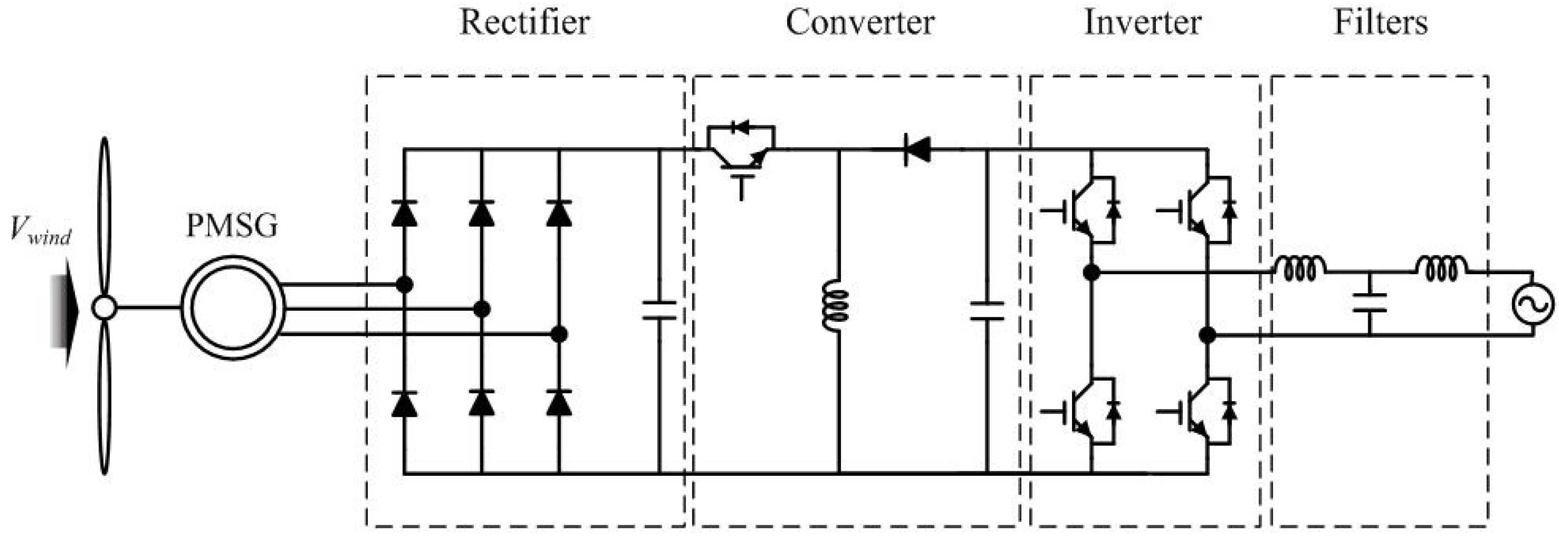
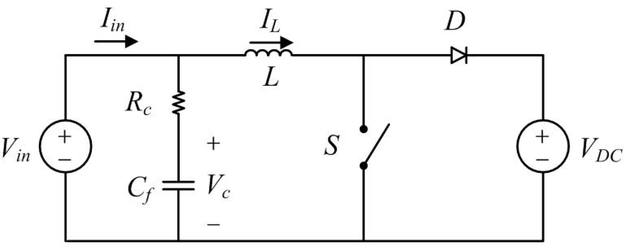
2. Controller Design for Wind Power Systems


3. MPPT Method
3.1. MPPT Method Using TSR Control


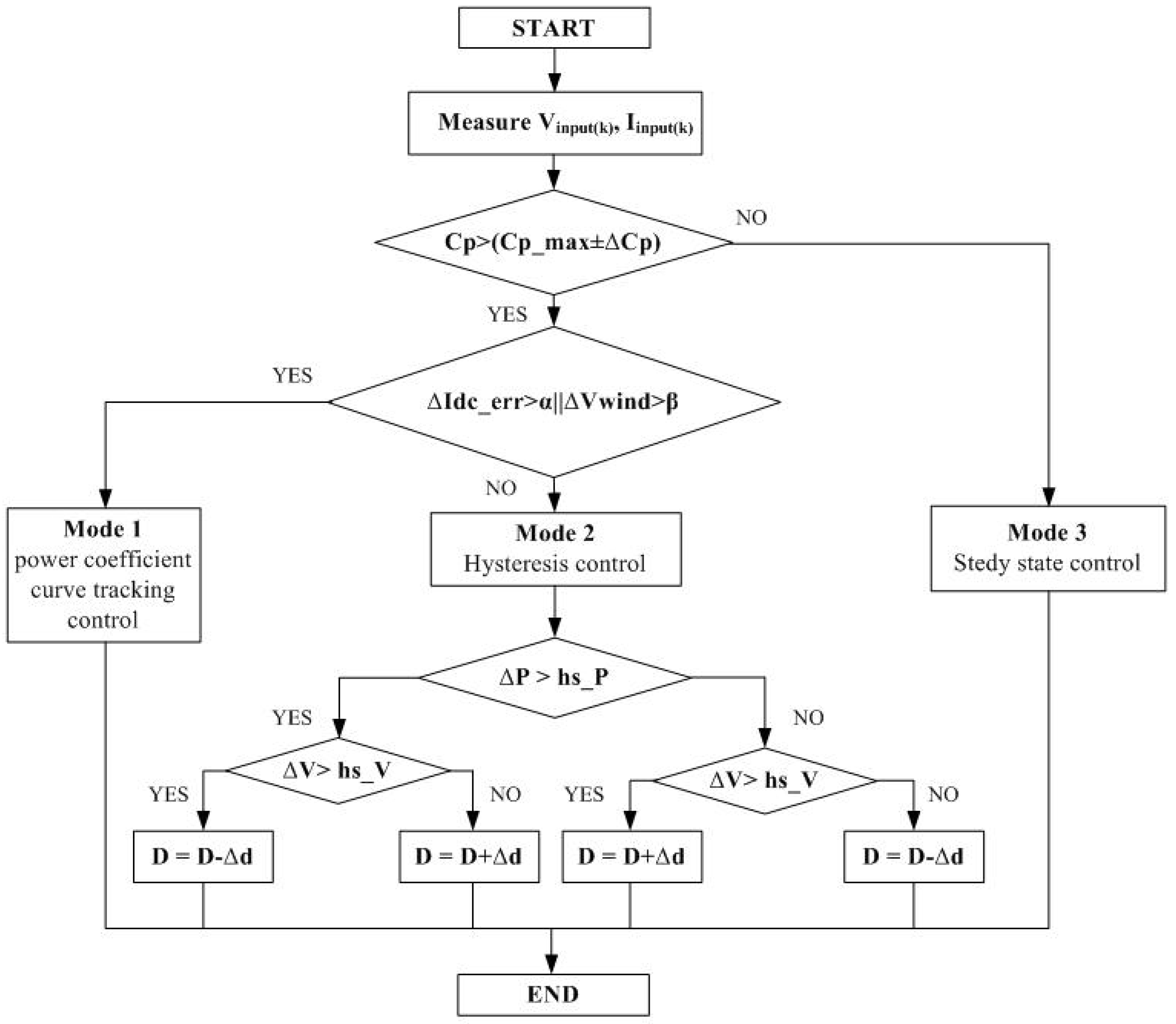
3.2. Proposed MPPT Method with Hysteresis Control


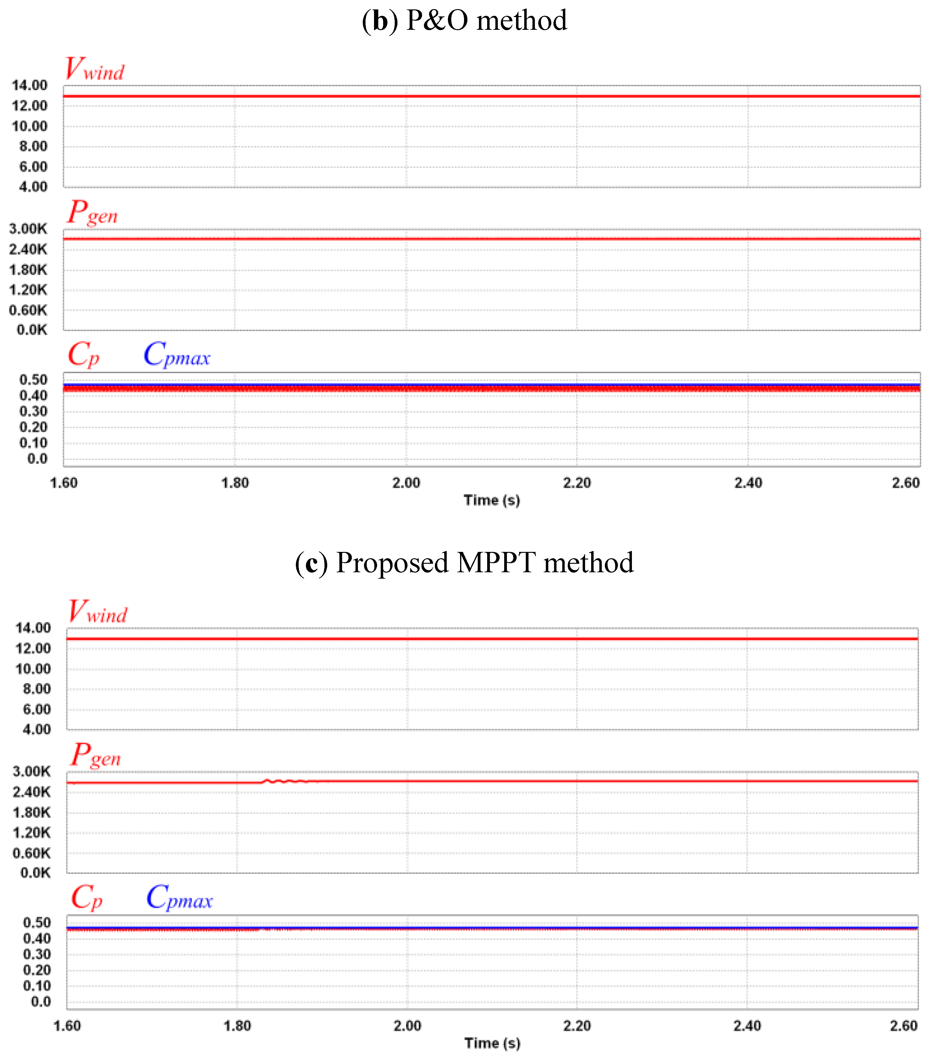
4. Simulations

| DC-link voltage | 400 V |
| Boost inductance | 6 mH |
| Control period | 100 μs |
| Changes in wind speed | 5 to 13 m/s |
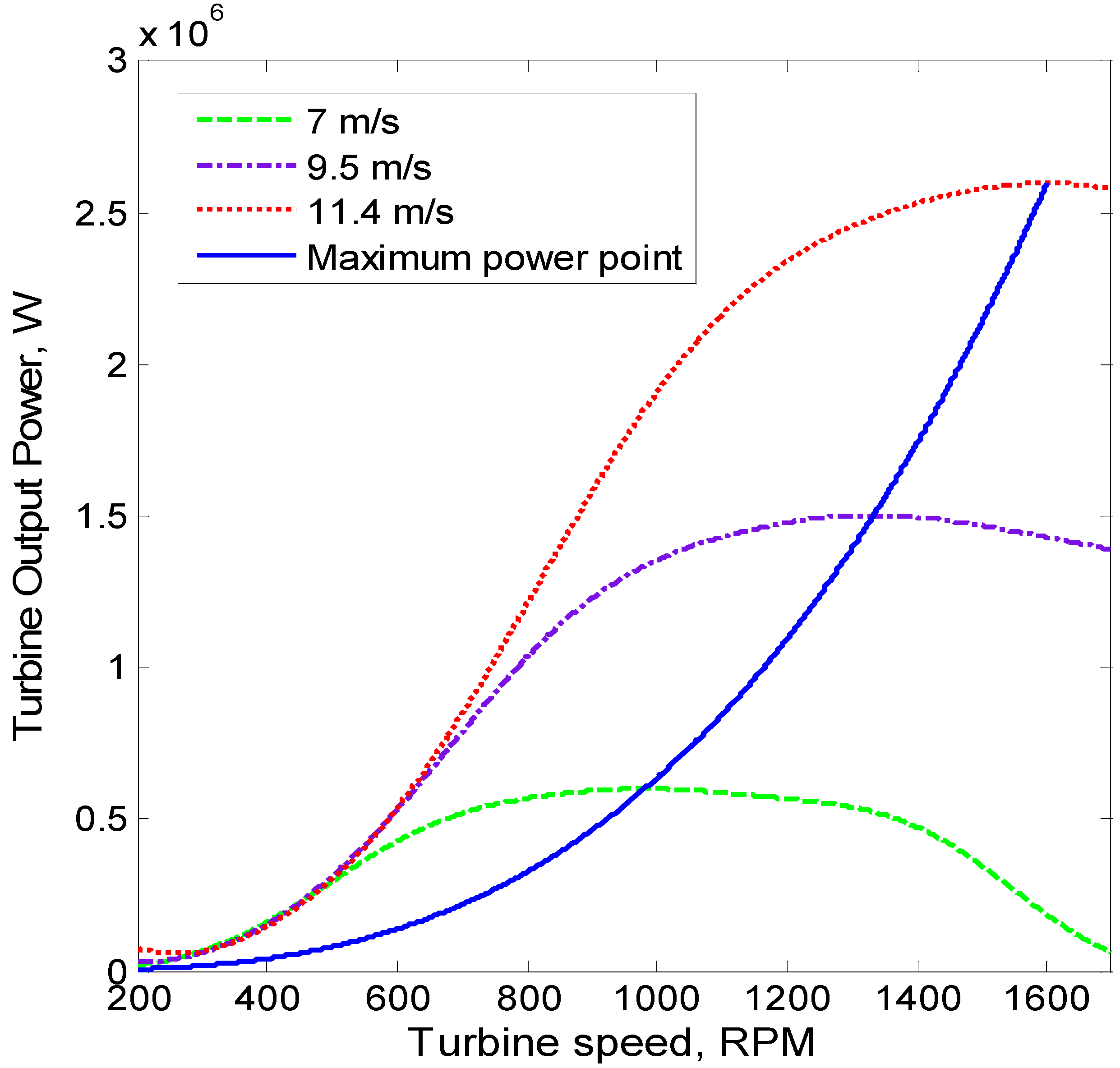
| Cp_max | 0.475 |
| TSRopt | 2.9531 |


5. Experimental
| Paramerter | Value | |
| Rated power | 3 kW | |
| Rated current (grid side) | 13.5 Arms | |
| DC-link voltage | 350 Vdc | |
| Grid voltage | Single phase 220 Vrms | |
| Switching frequency | 5 kHz | |
| Boost converter | L1 | 3 mH |
| C1 | 1100 μF | |
| LCLfilter | L2 | 3.5 mH |
| L3 | 2.5 mH | |
| C2 | 10 μF | |


6. Conclusions
Acknowledgments
References
- Jeong, H.G.; Lee, K.B.; Choi, S.W.; Choi, W.J. Performance improvement of LCL-filter based grid connected-inverters using PQR power transformations. IEEE Trans. Power Electron. 2010, 25, 1320–1330. [Google Scholar] [CrossRef]
- Lee, J.S.; Jeong, H.G.; Lee, K.B. Active damping for wind power systems with an LCL filter using a DFT. J. Power Electron. 2012, 12, 326–332. [Google Scholar] [CrossRef]
- Kortabarria, I.; Andreu, J.; Martinez, D.A.; Ibarra, E.; Robles, E. Maximum power extraction algorithm for a small wind turbine. In Proceedings of Power Electronics and Motion Control, Ohrid, Macedonia, 6–8 September 2010; pp. 12–54.
- Mirecki, A.; Roboam, X.; Richardeau, F. Architecture complexity and energy efficiency of small wind turbines. IEEE Trans. Ind. Electron. 2007, 54, 660–670. [Google Scholar] [CrossRef]
- Chwa, D.K.; Lee, K.B. Variable structure control of the active and reactive powers for a DFIG in wind turbines. IEEE Trans. Ind. Appl. 2010, 46, 2545–2555. [Google Scholar] [CrossRef]
- Park, K.W.; Lee, K.B. Hardware simulator development for a 3-parallel grid-connected PMSG wind power system. J. Power Electron. 2010, 10, 555–562. [Google Scholar] [CrossRef]
- Kazmi, S.M.R.; Goto, H.; Guo, H.J.; Ichinokura, O. A novel algorithm for fast and efficient speed-sensorless maximum power point tracking in wind energy conversion systems. IEEE Trans. Ind. Electron. 2011, 58, 29–36. [Google Scholar] [CrossRef]
- Pan, T.; Ji, Z.; Jiang, Z. Maximum power point tracking of wind energy conversion systems based on sliding mode extremum seeking control. In Proceedings of IEEE Energy 2030, Atlanta, GA, USA, 17–18 November 2008; pp. 1–5.
- Nguyen, T.H.; Lee, D.C. Improved LVRT capability and power smoothening of DFIG wind turbine systems. J. Power Electron. 2011, 11, 568–575. [Google Scholar] [CrossRef]
- Ahmed, T.; Nishida, K.; Nakaoka, M. Wind power grid integration of an IPMSG using a diode rectifier and a simple mppt control for grid-side inverters. J. Power Electron. 2010, 10, 548–554. [Google Scholar] [CrossRef]
- Kazmi, S.M.R.; Goto, H.; Guo, H.J.; Ichinokura, O. A novel algorithm for fast and efficient speed-sensorless maximum power point tracking in wind energy conversion systems. IEEE Trans. Ind. Electron. 2011, 58, 29–36. [Google Scholar] [CrossRef]
- Hohm, D.P.; Ropp, M.E. Comparative study of maximum power point tracking algorithms using an experimental, programmable, maximum power point tracking test bed. In Proceedings of Photovoltaic Specialists, Anchorage, AK, USA, 15–22 September 2000; pp. 1699–1702.
- Moor, G.D.; Beukes, H.J. Maximum power point trackers for wind turbines. In Proceedings of Power Electronics Specialist Conference (PESC), Aachen, Germany, 20–15 June 2004; pp. 2044–2049.
- Nakamura, T.; Morimoto, S.; Sanada, M.; Takeda, Y. Optimum control of IPMSG for wind generation system. In Proceedings of Power Conversion Conference (PCC), Osaka, Japan, 2–5 April 2002; pp. 1435–1440.
- Tse, K.K.; Ho, B.M.T.; Chung, H.S.-H.; Hui, S.Y.R. A comparative study of maximum-power-point trackers for photovoltaic panels using switching-frequency modulation scheme. IEEE Trans. Ind. Electron. 2004, 51, 410–418. [Google Scholar] [CrossRef]
- Hilloowala, R.M.; Sharaf, A.M. A rule-based fuzzy logic controller for a PWM inverter in a stand alone wind energy conversion scheme. IEEE Trans. Ind. Appl. 1996, 31, 57–65. [Google Scholar] [CrossRef]
- Chedid, R.; Mrad, F.; Basma, M. Intelligent control of class of wind energy conversion systems. IEEE Trans. Energy Convers. 1999, 14, 1597–1604. [Google Scholar] [CrossRef]
- Johnson, K.; Fingersh, L.; Balas, M.; Pao, L. Methods for increasing region 2 power capture on a variable speed wind turbine. J. Sol. Energy Eng. 2004, 126, 1092–1100. [Google Scholar] [CrossRef]
- Johnson, K.E.; Pao, L.Y.; Balas, M.J.; Fingersh, L.J. Control of variable-speed wind turbines: Standard and adaptive techniques for maximizing energy capture. IEEE Trans. Control Syst. Mag. 2006, 26, 70–81. [Google Scholar] [CrossRef]
- Jabr, H.M.; Dongyun, L.; Kar, N.C. Design and implementation of neuro-fuzzy vector control for wind-driven doubly-fed induction generator. IEEE Trans. Sustain. Energy 2011, 2, 404–414. [Google Scholar] [CrossRef]
© 2012 by the authors; licensee MDPI, Basel, Switzerland. This article is an open access article distributed under the terms and conditions of the Creative Commons Attribution license (http://creativecommons.org/licenses/by/3.0/).
Share and Cite
Jeong, H.G.; Seung, R.H.; Lee, K.B. An Improved Maximum Power Point Tracking Method for Wind Power Systems. Energies 2012, 5, 1339-1354. https://doi.org/10.3390/en5051339
Jeong HG, Seung RH, Lee KB. An Improved Maximum Power Point Tracking Method for Wind Power Systems. Energies. 2012; 5(5):1339-1354. https://doi.org/10.3390/en5051339
Chicago/Turabian StyleJeong, Hae Gwang, Ro Hak Seung, and Kyo Beum Lee. 2012. "An Improved Maximum Power Point Tracking Method for Wind Power Systems" Energies 5, no. 5: 1339-1354. https://doi.org/10.3390/en5051339