Determination of Steady-State and Faulty Regimes of Overhead Lines by Means of Multiconductor Cell Analysis (MCA)

Abstract

Single-phase positive sequence modelling is often used in power systems when power flows and short circuit analysis are assessed. Of course, the use of single-phase positive sequence modelling assumes purely three-phase configurations and perfectly symmetrical ones so that single-phase modelling considers that all the phase conductors behave in the same way. When considering the physical reality of power networks, this assumption can be questionable and the behaviors of all the system conductors including the passive ones (earth wires for overhead lines, metallic screens and armours for cables and enclosures for gas insulated lines) is completely unknown. Therefore, the present multiconductor cell analysis (MCA) becomes necessary, since it allows one to achieve great precision results on the regimes of both phase conductors and passive conductors. MCA offers a powerful tool in order to validate (or less) approximated and simplified computation methods. In particular, for single and double circuit overhead lines (OHLs), the current phasors induced in the earth wires and the ground return current alongside the line can be directly computed by MCA in steady state and faulty regimes. It is worth noting that, for faulty regimes, MCA allows also evaluating the approximation degree and validity field of screening factors k.

1. Introduction

Multiconductor cell analysis (MCA) takes advantage of the extensive use of the admittance matrices in order to consider any asymmetrical system with all the active and passive (earth wires for OHLs, screens and armors for underground insulated cables (UGCs), enclosures for gas insulated lines (GILs), keraunic wires, buried conductors, rails, feeders, overhead contact line with catenary suspension for AC high speed railway systems) conductors. It allows knowing directly the electrical behaviors of all the electrical quantities alongside an OHL. In the following, the steady state regime and the faulty regime of OHLs are considered. Furthermore a comparison between MCA and the commercial software EMTP-RV results is presented, which has given a very good agreement.

2. Application of MCA to Overhead Lines

MCA has been already applied to a great number of asymmetrical systems: cross-bonded underground insulated cables [1,2], shunt compensated ones, distribution line carrier, solid bonded or multiple-point bonded gas insulated lines [3], Milliken type EHV insulated cables. In this paper a thorough exposition of the application of MCA to overhead lines is presented. It allows considering:

(1)

Single or double circuit in electrical parallel with any type of phasing (low reactance or super bundle ones);

(2)

Any tower type, with different earth resistivities along the line and different tower resistances;

(3)

The steady-state regime of an OHL supplying a balanced (or not) three-phase load;

(4)

Faulty regimes (line-to-earth, line-to-line, line-to-line-to-earth, three phase short-circuit), with two end substations each characterized by its own fault levels.

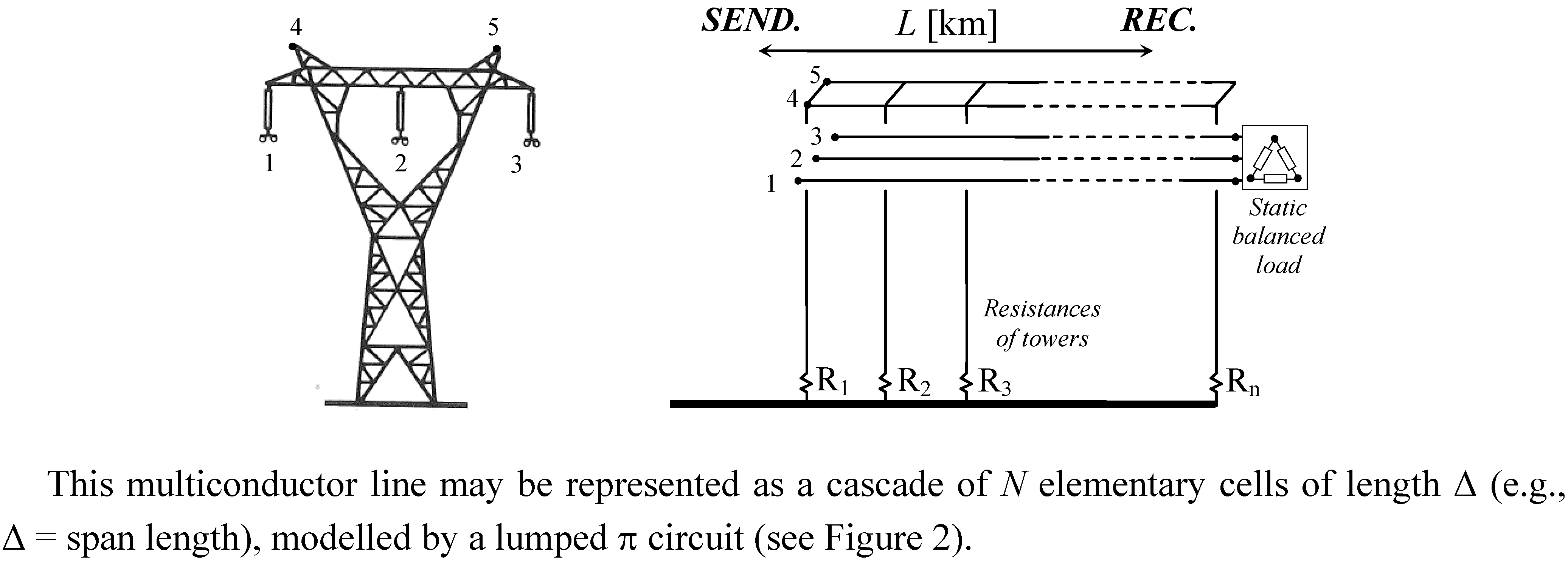
For the sake of a clear explanation, let us consider a single-circuit OHL composed of five conductors (n = 5; see Figure 1) parallel to themselves and to the ground: 1, 2, 3 are the phase conductors (in Figure 1, bundle ones) and 4, 5 are the earth wires.

Figure 1. Multiconductor representation of OHL supplying a static balanced load; SEND—sending-end; REC—receiving-end.

Figure 1. Multiconductor representation of OHL supplying a static balanced load; SEND—sending-end; REC—receiving-end.

This multiconductor line may be represented as a cascade of N elementary cells of length Δ (e.g., Δ = span length), modelled by a lumped π circuit (see Figure 2).

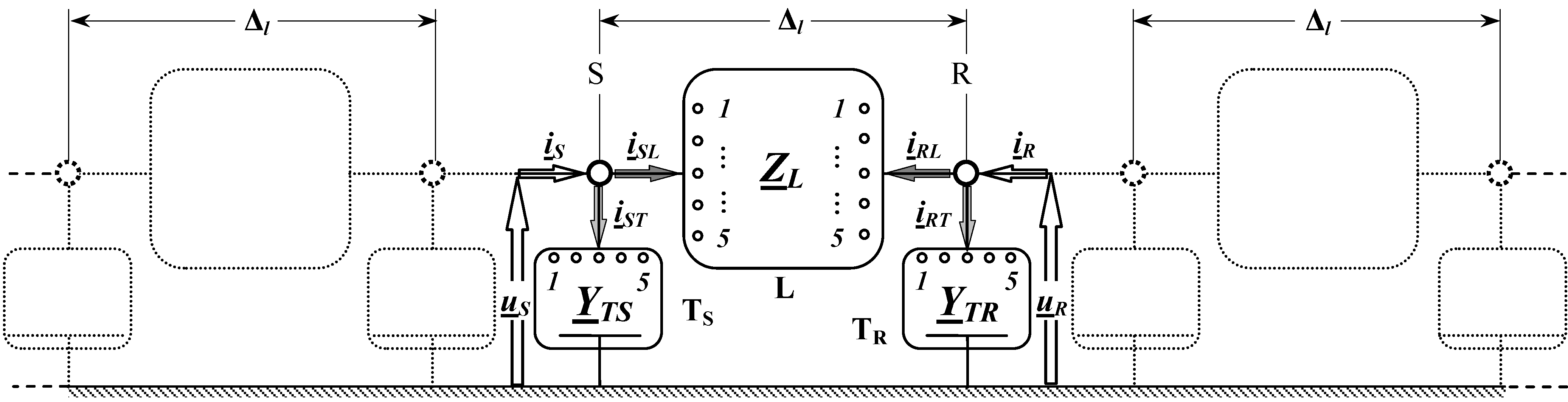
Figure 2. Cascade of N elementary cells for OHL modelling.

Figure 2. Cascade of N elementary cells for OHL modelling.

Being Δ sufficiently small, it is possible to lump distributed shunt admittances at the ends of the cell (Y_TS and Y_TR are the transverse blocks), thus allowing the separate study of longitudinal elements. In order to form Z_L, it is necessary to compute the self and mutual longitudinal impedances, which account for the earth return currents. They can be obtained by applying the simplified Carson-Clem formulae [4] or the complete Carson formulae [5] with Carson’s corrections in terms of series [6]. It has been widely demonstrated by one of the authors that at power frequency (50 or 60 Hz) the Carson-Clem formulae are very precise and consequently they are a powerful tool so giving the same results of complete Carson ones (Section 5).

In order to give the above mentioned sentence a theoretical justification, the simplified Carson-Clem formulae can be licitly applied if the spacing between conductors d_i,j ≤ 0.135D_e when $D_e=658\cdot \sqrt{\rho /f}$ [m] “Carson Depth”; ρ = electrical resistivity of the soil [Ωm]; f = power frequency (50–60 Hz). By supposing f = 50 Hz and a low earth resistivity e.g., 10 Ωm, it yields:

$$D_e=658\sqrt{\frac{\rho }{f}}=658\sqrt{\frac{10}{50}}=294\left[\text{m}\right]$$

(1)

The spacings between phases in OHL are never greater than 40 m, therefore it is rather unlikely to have the condition d_i,j > 0.135D_e $\cong$ 40 m even with very low resistive earth; hence the Carson-Clem formulae can be always used. With great mutual spacings between phases belonging to different circuits in the same corridor, the complete Carson formulae must be used. The self and mutual impedances by means of Carson-Clem formulae are given by:

$${\underset{¯}{z}}_{i,i}=r_i+{\text{π}}^2\cdot {10}^{-4}\cdot f+j4\text{π}\cdot {10}^{-4}\cdot f\cdot \ln \left(\frac{2\cdot D_e}{{d^{\prime }}_i}\right)\text{}\left[\text{Ω/km}\right]$$

(2)

$${\underset{¯}{z}}_{i,j}={\text{π}}^2\cdot {10}^{-4}\cdot f+j4\text{π}\cdot {10}^{-4}\cdot f\cdot \ln \left(\frac{D_e}{d_{i,j}}\right)\left[\text{Ω/km}\right]$$

(3)

where r_i = kilometric resistance of conductor i [Ω/km] (if bundle conductor with n subconductors per phase $r_i=r_{i\_sub}/n$); d_i′ = 2·GMR = k″d [m] (GMR = Geometrical Mean Radius) where k′′ are listed in tables depending upon the composition of the conductor and d [m] is the diameter of the conductor (if bundle conductor:

$$d_i´=2\cdot \sqrt[n]{n\cdot k″\cdot \frac{d_{sub}}{2}\cdot R_{circle}^{n-1}}$$

where R_circle [m] is the radius of the circle on which the subconductors lay and d_sub [m] is the diameter of the subconductors); d_i,j = distance between conductor i and j [m]. Once z_i,i and z_i,j have been computed, it is possible to form the matrix Z_L (5 × 5) and to characterize, by means of Equation (4) the steady state regime of longitudinal block L of Figure 2 (where all voltage and current vectors are shown):

$${\underset{¯}{\mathit{u}}}_S-{\underset{¯}{\mathit{u}}}_R={\underset{¯}{\mathit{Z}}}_L{\underset{¯}{\mathit{i}}}_{SL}$$

(4)

and by considering the evident relation Equation (5):

$${\underset{¯}{\mathit{i}}}_{SL}=-{\underset{¯}{\mathit{i}}}_{RL}$$

(5)

it yields:

$${\underset{¯}{\mathit{Z}}}_L^{-1}{\underset{¯}{\mathit{u}}}_S-{\underset{¯}{\mathit{Z}}}_L^{-1}{\underset{¯}{\mathit{u}}}_R={\underset{¯}{\mathit{i}}}_{SL}$$

(6)

$$-{\underset{¯}{\mathit{Z}}}_L^{-1}{\underset{¯}{\mathit{u}}}_S+{\underset{¯}{\mathit{Z}}}_L^{-1}{\underset{¯}{\mathit{u}}}_R={\underset{¯}{\mathit{i}}}_{RL}$$

(7)

The Equations (6,7) can be written in an elegant matrix form as:

(8)

The matrix Y_LΔ (10 × 10) is the admittance matrix regarding block L circuit formed by five longitudinal links.

The shunt capacitive matrix computation can be obtained from Maxwell potential coefficient matrix. Its elements are easy to compute from the tower geometry and from the conductor radii [7]. It is worth remembering that the average heights of conductors can be used by means of Equation (9):

$$h_{average}=h_{tower}-\frac{2}{3}\cdot sag\left[\text{m}\right]$$

(9)

where h_tower is the conductor height at tower.

Then, as already mentioned, the shunt capacitive and conductive links are divided into two halves and lumped at the ends of the elementary cell. The capacitive susceptances (of half cell) between each conductor are considered in the (5 × 5) matrix Y_TS = Y_TR. The vectors of the shunt currents at both ends of the cell are (see Figure 2):

(10)

Hence the steady state regime of the elementary cell is represented by Y_Δ which is the superimposition of Y_LΔ and Y_TΔ:

(11)

2.1. Steady State Regime of Single Circuit EHV OHL

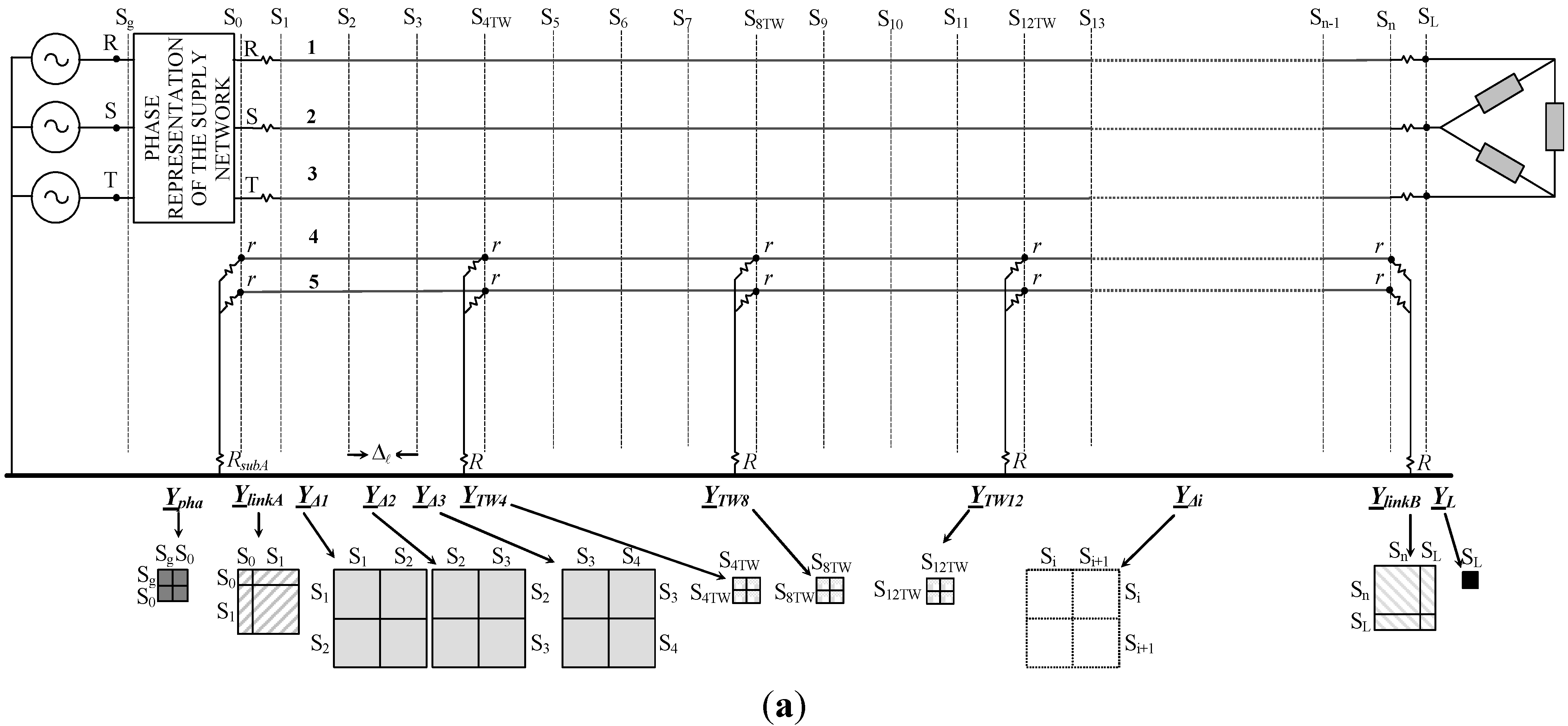
In order to achieve a complete analysis of an overhead line it is necessary to obtain the admittance matrix Y of the whole multiconductor system shown in Figure 3 (where S_g, S₀,…. S_L indicate the sections or ports). 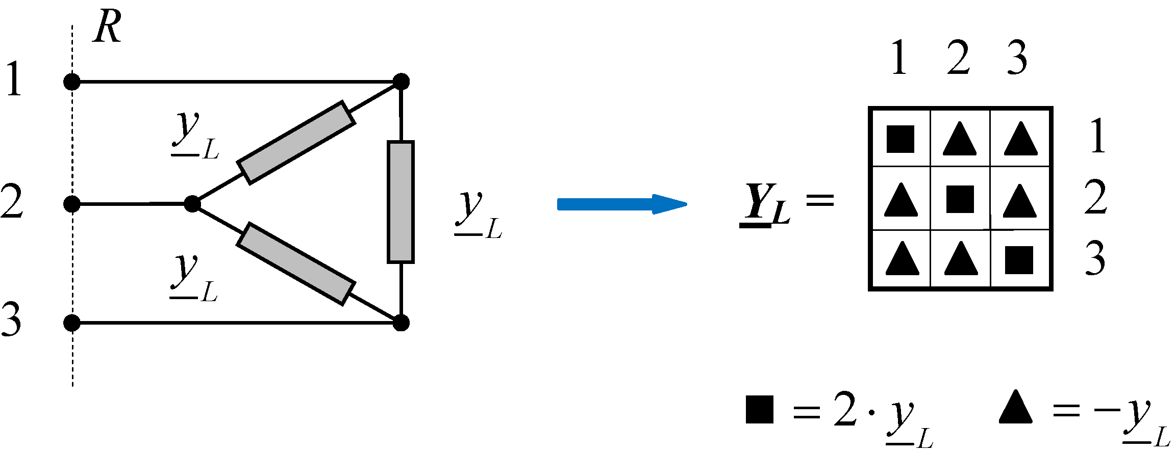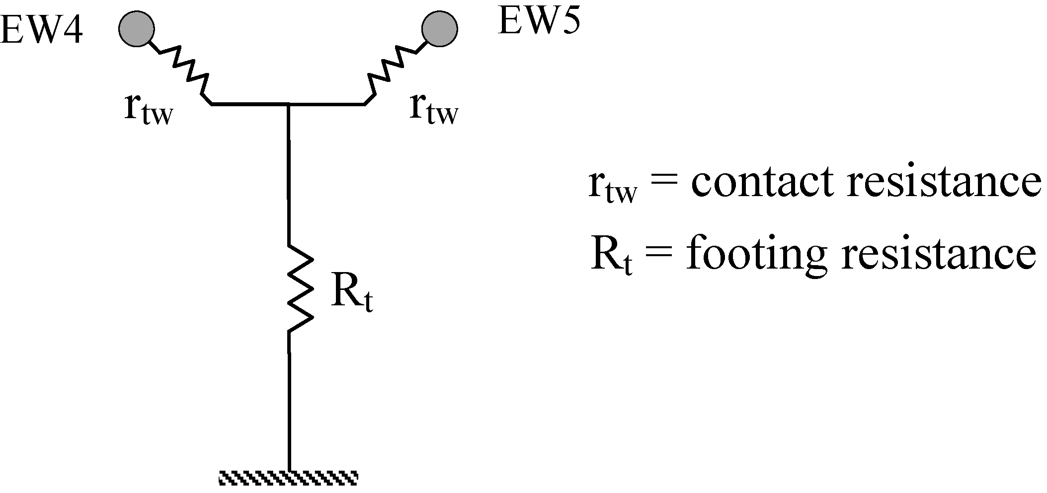This involves all the elements of the line which can be represented by their admittance matrix: (by starting from the left side) the equivalent supply network matrix Y_pha (3 × 3) (see Appendix I), the load matrix Y_L (3 × 3) (see Appendix II), the tower matrix Y_TW (2 × 2) (see Appendix III), and, of course, the already mentioned elementary cell matrices Y_Δi. In short-circuit occurrence (Section 4), the equivalent substation impedance Y_SUB (3 × 3) and fault matrix Y_fault (see Appendix IV) must be considered.

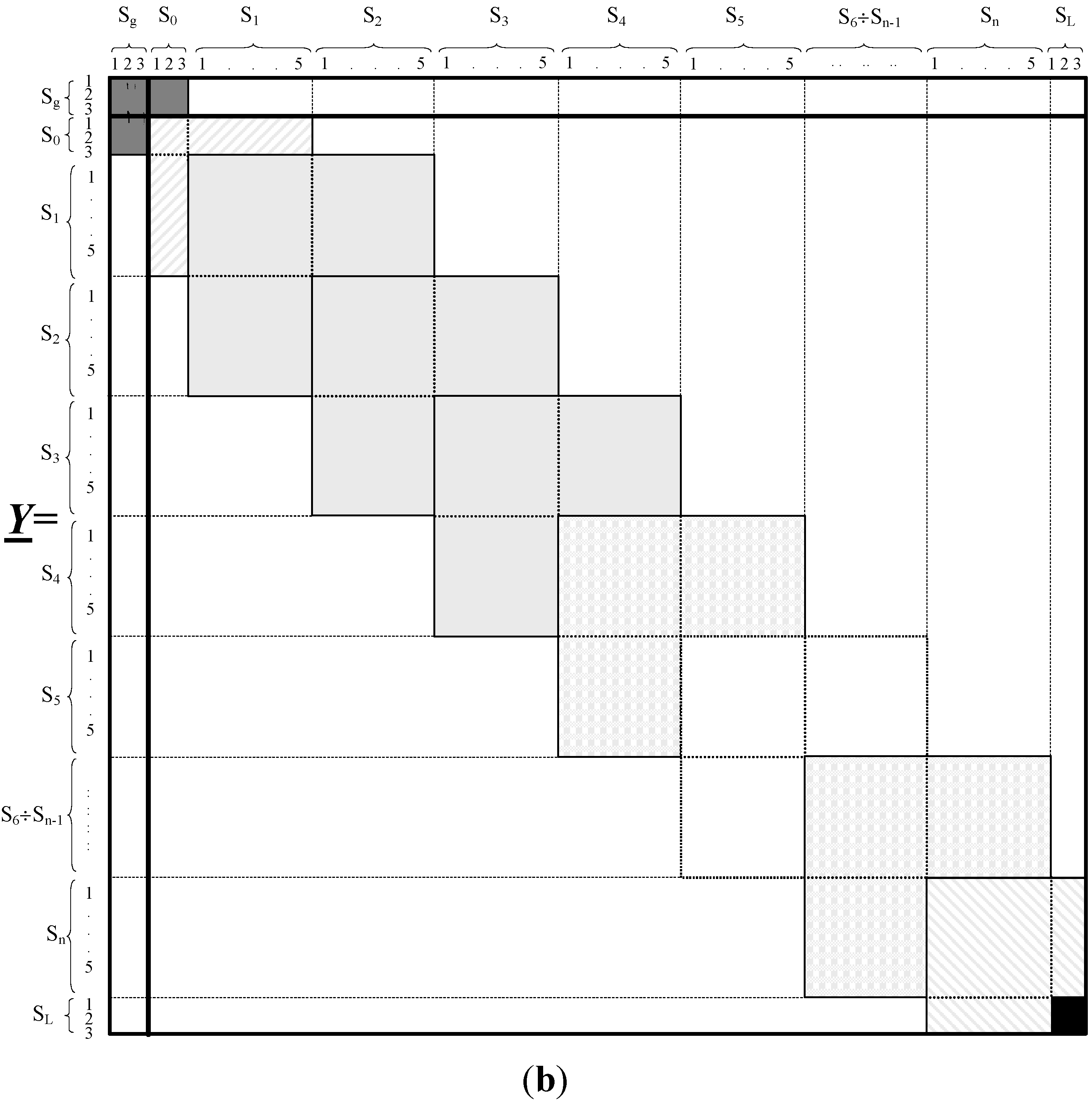
On the basis of the equation which leads to the general formulation of the current vectors injected in the different ports of the system (S_g, S₀,…. S_L), it can be ascertained that the admittance matrix Y is formed by partial overlapping ("tile style") of the above mentioned matrices as shown in Figure 3b. The resulting admittance matrix Y can be of large dimensions (depending upon the ratio OHL length/Δ_l) but it can be easily managed because of it is structurally sparse. Anyway, the use of the admittance frame of reference allows introducing easily local modifications of the system structure without reconstructing its entire matrix.

Figure 3. (a) Single circuit overhead line; (b) Structure of the matrix Y.

Figure 3. (a) Single circuit overhead line; (b) Structure of the matrix Y.

If the modification is between two sections, it is sufficient to substitute the matrix representing the modification for that existing before. If the modification is derived from a section, the matrix representing the modification must be superimposed in that section (e.g. the tower presence anywhere along the OHL). In fact, they can be represented by their admittance matrices which must be superimposed in the right location of matrix Y so to give a new total matrix Y_TOT.

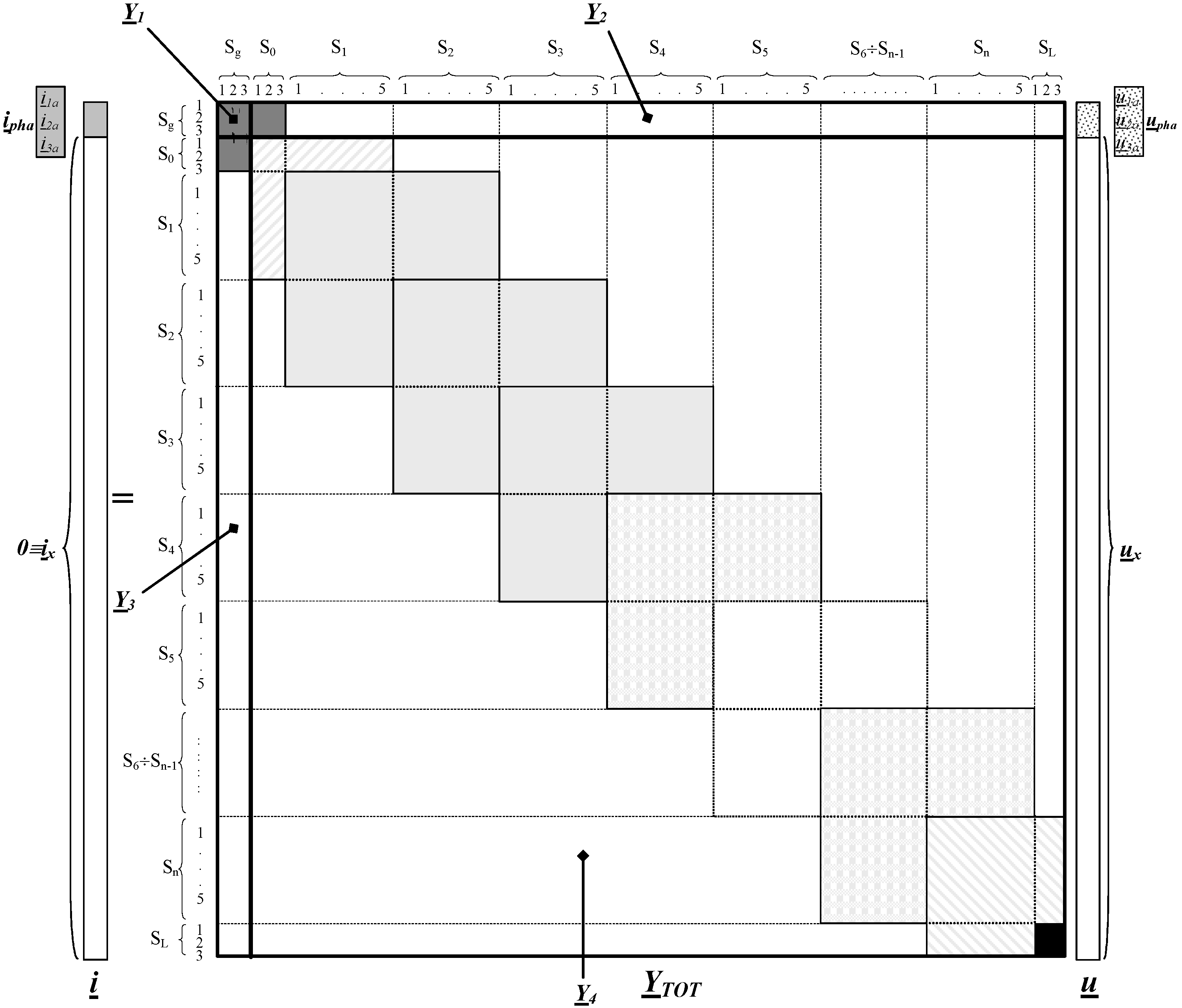
2.2. Steady State Matrix Solution of Multiconductor System

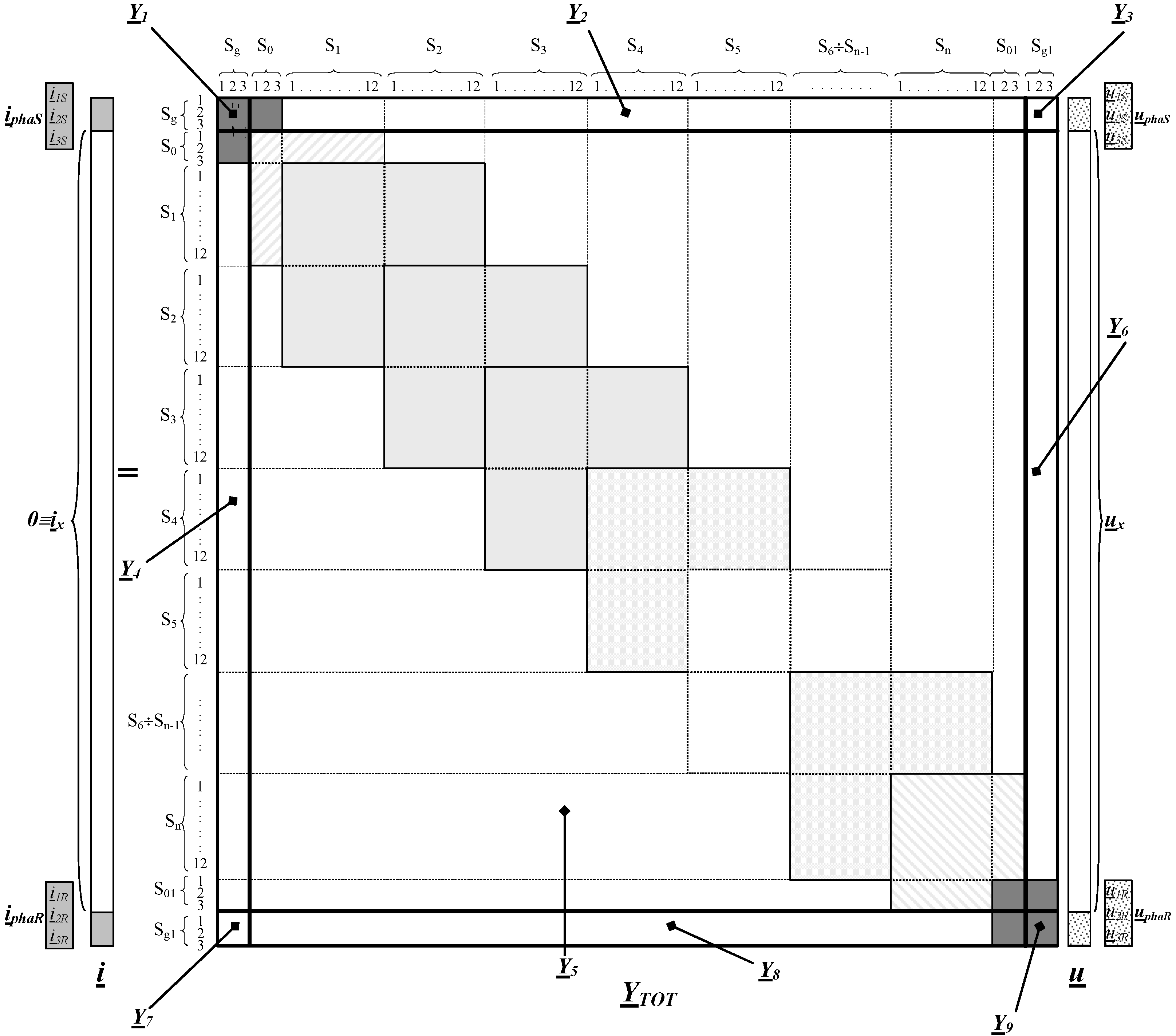
For the system of Figure 3b, the general equation i = Y_TOT u can be partitioned as in Figure 4. It is worth noting that only i_pha is a non zero current vector whereas i_x ≡ 0 so that it yields:

$${\underset{¯}{\mathit{i}}}_x\equiv 0={\underset{¯}{\mathit{Y}}}_3{\underset{¯}{\mathit{u}}}_{pha}+{\underset{¯}{\mathit{Y}}}_4{\underset{¯}{\mathit{u}}}_x$$

(12)

and thus:

$${\underset{¯}{\mathit{u}}}_x=-{\underset{¯}{\mathit{Y}}}_4^{-1}{\underset{¯}{\mathit{Y}}}_3{\underset{¯}{\mathit{u}}}_{pha}$$

(13)

where Y₄ is not singular and u_pha is fixed. So by knowing the subvector u_x the steady state regime of any cell, and hence of the whole multiconductor system, is completely available without iterations.

Figure 4. Partitioned matrix of i = Y_TOTu.

Figure 4. Partitioned matrix of i = Y_TOTu.

The inversion of Y₄ in Equation (13) could give computational drawbacks, but even if Y₄ is of great dimensions (i.e., with great number of N cells), its inversion can benefit from the partition in submatrices [8] and the use of parallel computing.

3. Application to HV OHL on Steady State Regime

The proposed multiconductor algorithms are applied to a 275 kV 2 × 400 mm² single circuit aluminum conductor steel reinforced (ACSR) OHL (Figure 5), whose geometrical and electrical characteristics are reported in Table 1.

Figure 5. Single circuit OHL tower arrangement.

Figure 5. Single circuit OHL tower arrangement.

Table 1. OHL geometrical and electrical characteristics.

Overhead line	Symbol	Unit	Value
Voltage level	-	kV	275
Line length	-	km	55.632
Span length	-	km	0.366
Earth resistivity (assumed equal along the line)	-	Ω m	100
Symmetrical loading at receiving end	-	MW + j Mvar	508.8 + j 103.32
Substation earthing resistance	-	Ω	0.1
Tower earthing resistance (assumed equal for all the tower)	-	Ω	10
Conductor diameter (bundle conductor)	-	mm	2 sub-cond. ACSR Lynx Ф = 19.53 mm
Per unit length resistance at 75° operation (50 Hz)	R	mΩ/km	96.10
Per unit length series inductance	l	mH/km	1.1051
Per unit length shunt leakance (50 Hz)	gav	nS/km	44.5
Per unit length capacitance	c	μF/km	0.010215
Ampacity referred to winter rating [9]	Ia	A	545 × 2
Winter rating [9]	-	MVA	519.2

Table 1. OHL geometrical and electrical characteristics.

Overhead line	Symbol	Unit	Value
Voltage level	-	kV	275
Line length	-	km	55.632
Span length	-	km	0.366
Earth resistivity (assumed equal along the line)	-	Ω m	100
Symmetrical loading at receiving end	-	MW + j Mvar	508.8 + j 103.32
Substation earthing resistance	-	Ω	0.1
Tower earthing resistance (assumed equal for all the tower)	-	Ω	10
Conductor diameter (bundle conductor)	-	mm	2 sub-cond. ACSR Lynx Ф = 19.53 mm
Per unit length resistance at 75° operation (50 Hz)	R	mΩ/km	96.10
Per unit length series inductance	l	mH/km	1.1051
Per unit length shunt leakance (50 Hz)	gav	nS/km	44.5
Per unit length capacitance	c	μF/km	0.010215
Ampacity referred to winter rating [9]	Ia	A	545 × 2
Winter rating [9]	-	MVA	519.2

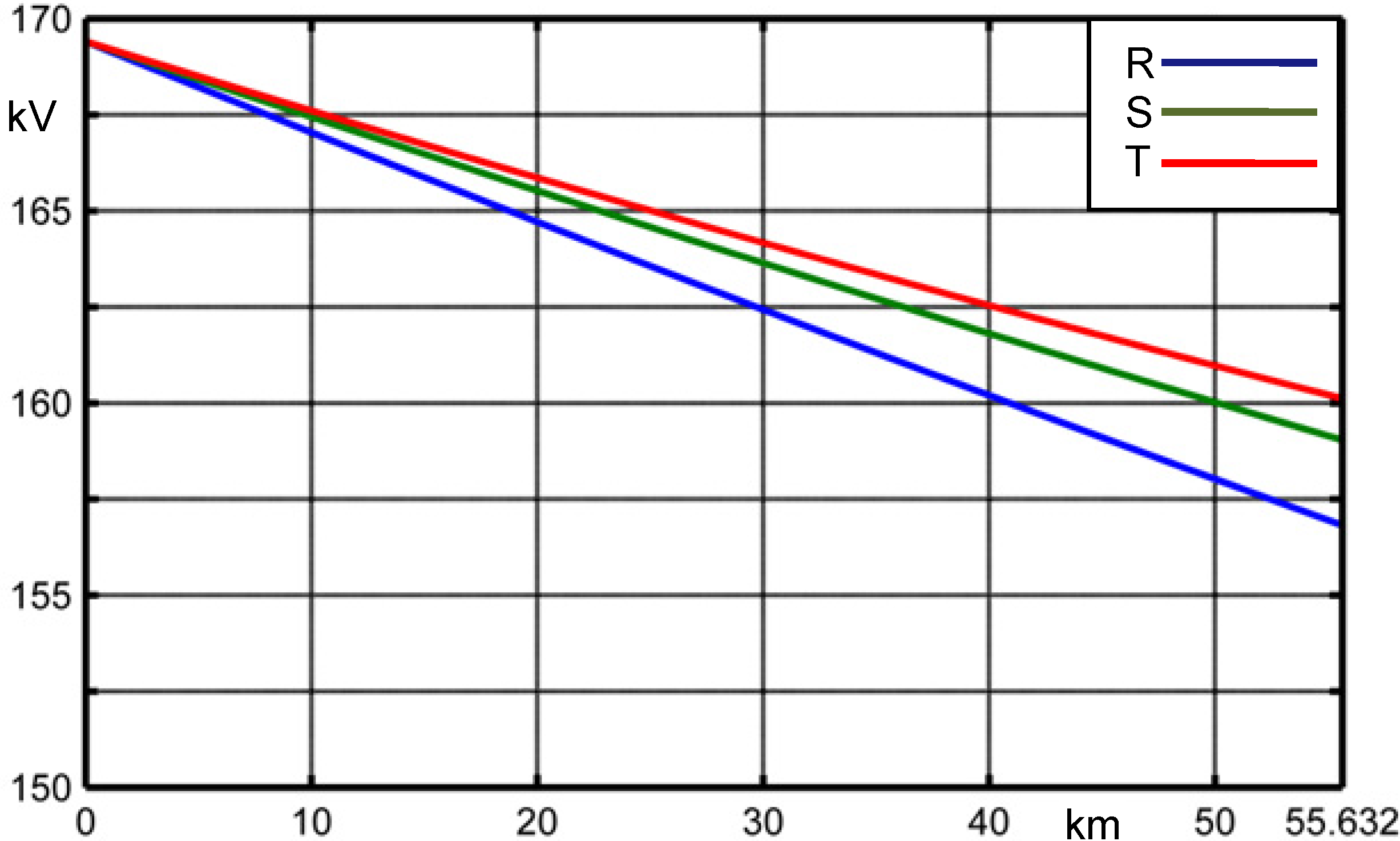
By means of the procedures of Section 2.2 it is possible to completely know the steady state behaviors of the electrical quantities along the line. Figure 6 shows the phase voltage behaviors along the line. There is a voltage drop which is different from phase to phase due to the asymmetrical nature of the un-transposed OHL.

Figure 6. Line-to-earth voltage magnitudes along the OHL.

Figure 6. Line-to-earth voltage magnitudes along the OHL.

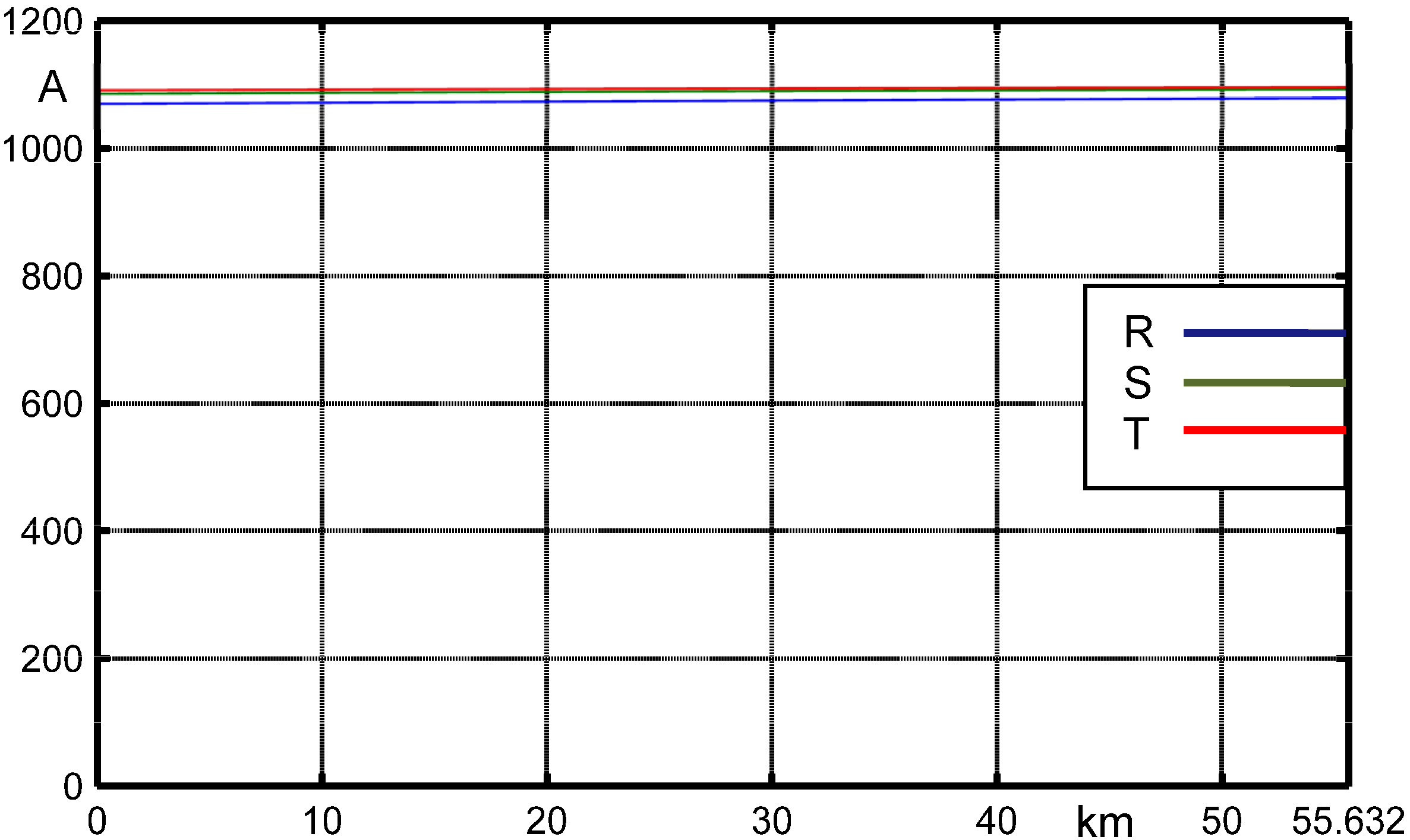
The phase current magnitudes are almost constant along the line ($\cong$ 1090 A) (see Figure 7) due to the very low capacitive susceptance of OHL. The earth wire voltage along the line is almost null (see Figure 8). This is a confirmation that it is licit to use the elimination technique of grounded conductors.

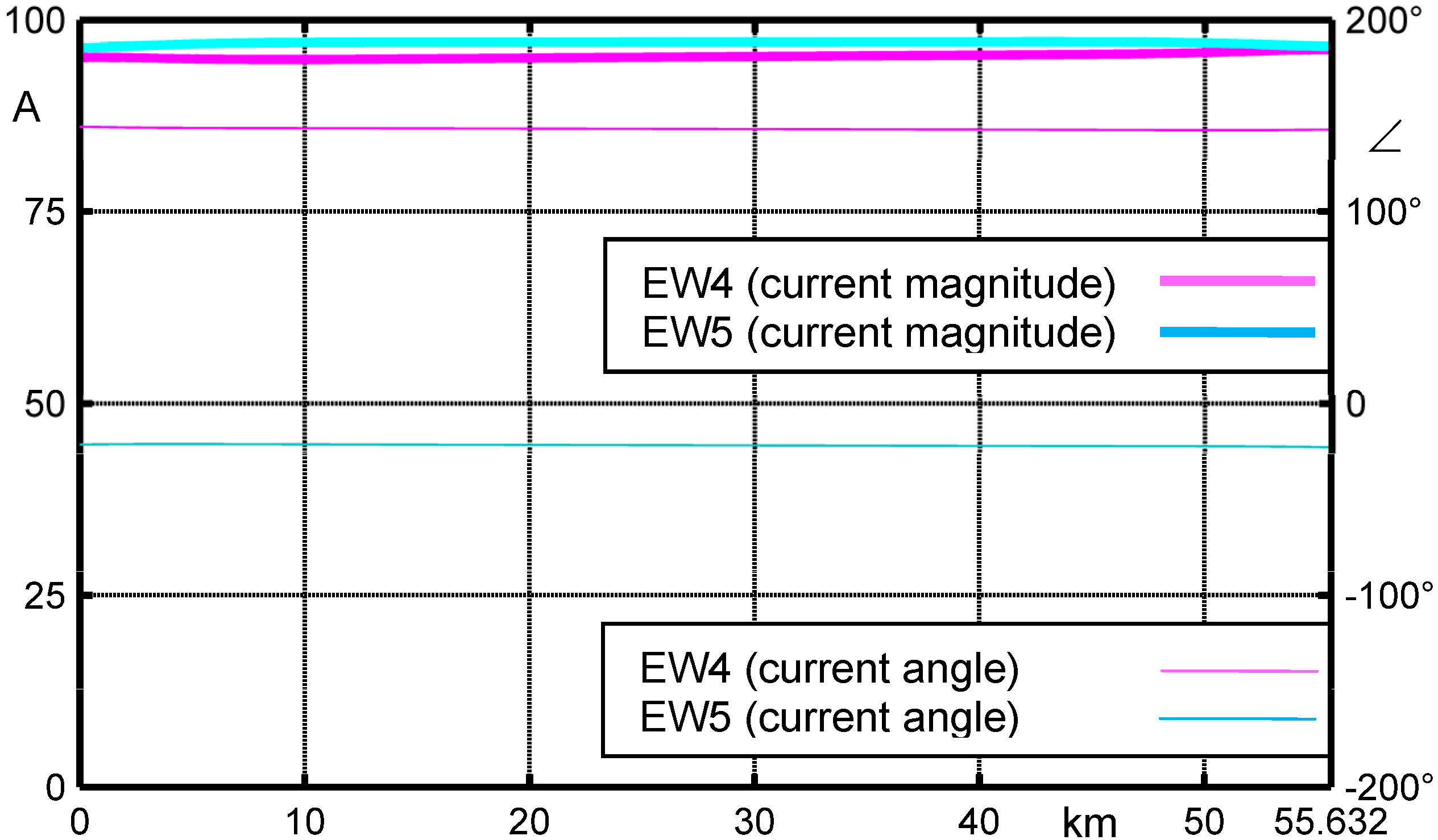
It is meaningful to observe that, even in steady state regime, both the induced currents in the earth wires and the ground return current are not negligible. The earth wire induced current magnitudes along the line have an almost constant value of 96 A (see Figure 9).

Figure 7. Phase current magnitudes along the OHL.

Figure 7. Phase current magnitudes along the OHL.

Figure 8. Earth wire voltage magnitudes along the OHL.

Figure 8. Earth wire voltage magnitudes along the OHL.

Figure 9. Earth wire current magnitudes (left axis) and angles (right axis) along the OHL.

Figure 9. Earth wire current magnitudes (left axis) and angles (right axis) along the OHL.

One of the most important features of MCA is that it allows directly achieving the ground return current. Since MCA can compute all the conductor current phasors in each section, I_GR is given by the 1st Kirchhoff’s Law:

$$\underset{¯}{I}GR+{\displaystyle \sum _{x=1}^n\underset{¯}{I}x}\equiv 0\Rightarrow \underset{¯}{I}GR=-{\displaystyle \sum _{x=1}^n\underset{¯}{I}x}$$

(14)

With the constant loading of Table 1 (S = 508.8 MW + j103.32 MVar), |I_GR |= 25 A (see Figure 10). This current could be responsible for ac metallic corrosion [10] and induced voltages on parallel metallic pipes buried in the neighborhood of OHL.

Figure 10. Ground return current magnitude and angle along the OHL.

Figure 10. Ground return current magnitude and angle along the OHL.

Another important result from MCA is the possibility to compute the whole power losses which are 19.269 MW. In order to roughly validate this value, it is possible to consider a constant current in the phase conductor equal to 1090 A so that the three-phase power losses result:

$$P_{J\_PH}=3\cdot r\cdot L\cdot I^2=3\cdot 0.0961\cdot 55.632\cdot {1090}^2=19.056\hspace{0.17em}\text{MW}$$

(15)

To these phase conductor power losses, the insulator and corona losses must be added so that it has:

$$P_{ins+cor}=g\cdot L\cdot U^2=0.18722MW$$

(16)

The power losses in the earth wires are not negligible and can be computed (by considering that the induced currents are 96 A constant along the line as in Figure 9) by means of:

$$P_{EW}=2\cdot r_{EW}\cdot L\cdot I_{EW}^2=2\cdot 0.1575\cdot 55.632\cdot {96}^2=0.1615\hspace{0.17em}\text{MW}$$

(17)

The whole power losses are given by the sum of the three abovementioned components i.e.:

$$P=P_{J\_PH}+P_{ins+cor}+P_{EW}=19.4047\hspace{0.17em}\text{MW}$$

(18)

which is in very good agreement with the power losses computed by MCA.

Comparison between the MCA and EMTP-RV

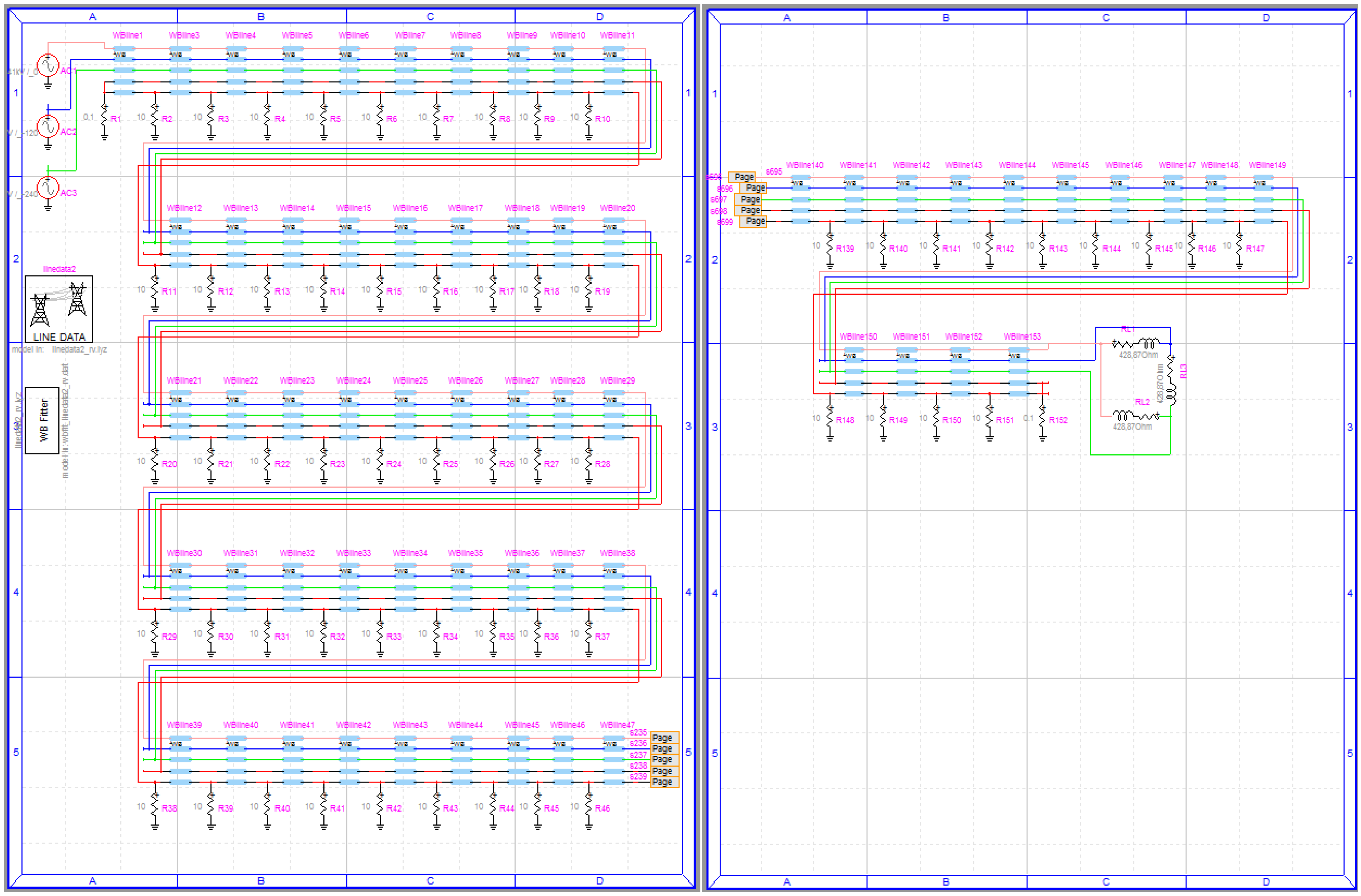
In this section some of the above presented MCA results are compared with the EMTP-RV results for the OHL of Section 3. The EMTP-RV electrical layout (the first and the last of four pages) is shown in Figure 11.

Figure 11. EMTP-RV single circuit OHL electrical layout (pages 1/4 and 4/4).

Figure 11. EMTP-RV single circuit OHL electrical layout (pages 1/4 and 4/4).

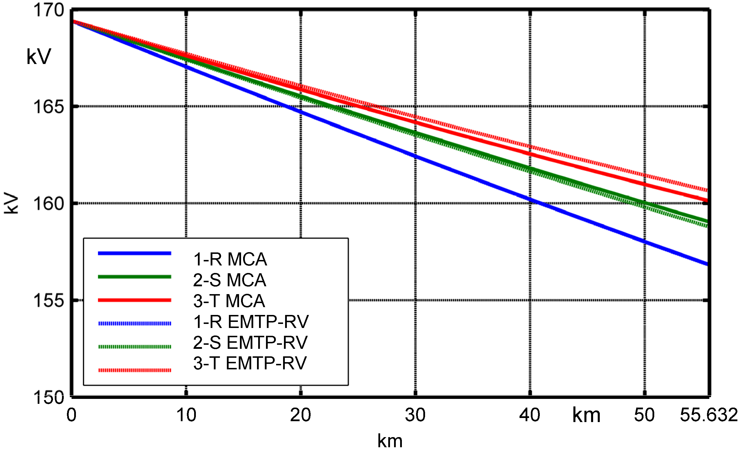
Figure 12 shows the phase voltage magnitude behavior along the single circuit OHL by means of MCA and EMTP-RV. The per cent voltage drops are reported in Table 2 where it infers that the maximum difference between the MCA and EMTP-RV is equal to 5.28%. The cpu-time in the simulation with MCA is 0.2087 s and with EMTP-RV is 0.3125 s (INTEL CORE 2 QUAD [email protected] GHz, 3.25 GB RAM).

Figure 12. Voltage magnitude comparison between MCA and EMTP-RV along the OHL.

Figure 12. Voltage magnitude comparison between MCA and EMTP-RV along the OHL.

Table 2. Single circuit OHL voltage drop comparison.

Eliminate	Voltage drop [%]
	Phase 1-R	Phase 2-S	Phase 3-T
MCA	7.4%	6.1%	5.49%
EMTP-RV	7.4%	6.26%	5.2%
Percentage difference	0.0%	2.62%	5.28%

Table 2. Single circuit OHL voltage drop comparison.

Eliminate	Voltage drop [%]
	Phase 1-R	Phase 2-S	Phase 3-T
MCA	7.4%	6.1%	5.49%
EMTP-RV	7.4%	6.26%	5.2%
Percentage difference	0.0%	2.62%	5.28%

In Table 2 “percentage difference” means:

$$100\cdot \frac{MCA-EMTPRV}{MCA}$$

(19)

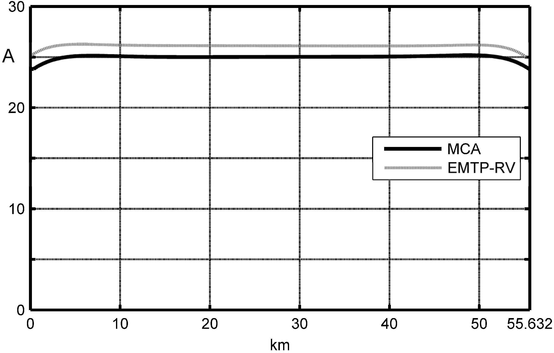
In Figure 13 the steady state |I_GR| for OHL of Section 3 is shown by using the MCA and EMTP-RV results. The maximum current difference is 1 A (4%).

Figure 13. Steady state ground return current magnitude comparison between the MCA and EMTP-RV.

Figure 13. Steady state ground return current magnitude comparison between the MCA and EMTP-RV.

4. Short-Circuit Analysis of Double-Circuit Overhead Line 400kV

In this section a double circuit OHL 400 kV 2 × 400 mm² ACSR, whose electrical and geometrical characteristics are reported in Table 3, has been studied on faulty regime by means of MCA (see Appendix IV). The tower arrangement is reported in Figure 14.

Table 3. Data assumed in the MCA for double-circuit OHL.

Overhead line	Symbol	Unit	Value
Voltage level	-	kV	400
Line length	-	km	135.42
Span length	-	km	0.366
Earth resistivity (assumed equal along the line)	-	Ω m	100
Symmetrical loading at receiving end	-	MW + j Mvar	2 × (2172.7 + j 441.2)
Substation earthing resistance	-	Ω	0.1
Tower earthing resistance(equal for all the towers)	-	Ω	10
Conductor diameter (bundle conductor)	-	mm2	4 sub-cond. ACSR Zebra Ф = 28.62 mm
Per unit length resistance at 25° (50 Hz)	r	mΩ/km	8.25
Per unit length series inductance	l	mH/km	0.4218
Per unit length shunt leakance (50 Hz)	gav	nS/km	33.56
Per unit length capacitance	c	μF/km	0.0266521
Ampacity referred to winter rating [11]	Ia	A	800 × 4
Winter rating [11] of double-circuit	MVA	-	2 × 2217

Table 3. Data assumed in the MCA for double-circuit OHL.

Overhead line	Symbol	Unit	Value
Voltage level	-	kV	400
Line length	-	km	135.42
Span length	-	km	0.366
Earth resistivity (assumed equal along the line)	-	Ω m	100
Symmetrical loading at receiving end	-	MW + j Mvar	2 × (2172.7 + j 441.2)
Substation earthing resistance	-	Ω	0.1
Tower earthing resistance(equal for all the towers)	-	Ω	10
Conductor diameter (bundle conductor)	-	mm2	4 sub-cond. ACSR Zebra Ф = 28.62 mm
Per unit length resistance at 25° (50 Hz)	r	mΩ/km	8.25
Per unit length series inductance	l	mH/km	0.4218
Per unit length shunt leakance (50 Hz)	gav	nS/km	33.56
Per unit length capacitance	c	μF/km	0.0266521
Ampacity referred to winter rating [11]	Ia	A	800 × 4
Winter rating [11] of double-circuit	MVA	-	2 × 2217

Figure 14. Tower characteristics of 400 kV double-circuit OHL in electric parallel with low reactance phasing.

Figure 14. Tower characteristics of 400 kV double-circuit OHL in electric parallel with low reactance phasing.

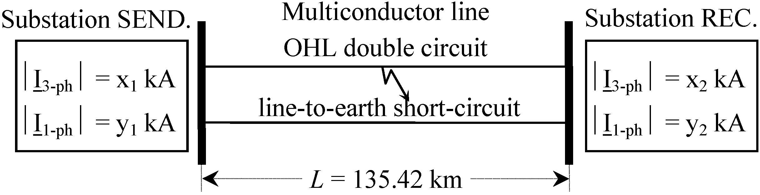
Let us suppose the fault occurring at midline (i.e., at 67.71 km from both ends) between one phase (e.g., 1R phase) and earth wire (line-to-earth short-circuit). It is worth remembering that in order to characterize the end substations it is necessary to know the fault levels (three-phase x₁, x₂ and single-phase y₁, y₂ sub-transient short circuit currents usually given by TSO) as in Figure 15.

Figure 15. Multiconductor line in short-circuit condition supplied by end substations.

Figure 15. Multiconductor line in short-circuit condition supplied by end substations.

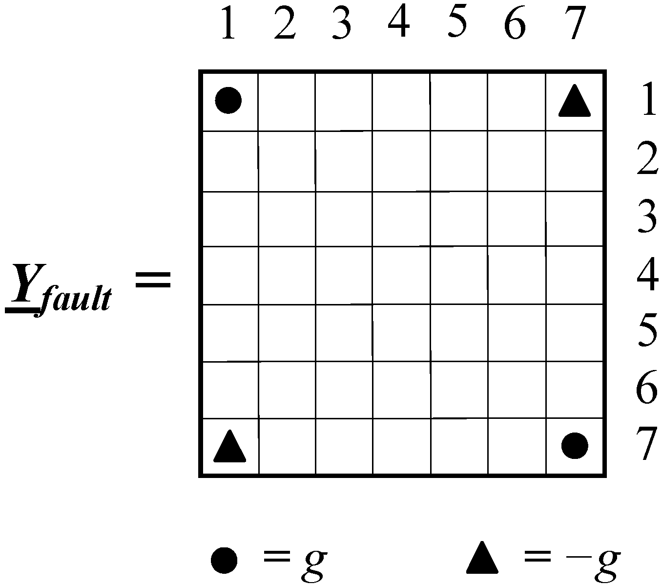
Once the fault levels are known, the equivalent sequence impedances and phase impedances of each substation can be computed by means of the procedure in Appendix I, in order to create the equivalent supply network matrix. The short-circuit between a phase and the earth wire can be considered by means of the matrix Y_fault reported in Appendix IV. In accordance with IEC 60909-0 [12], a voltage factor must be applied to the nominal line-to-earth voltage. Since maximum currents in HV and EHV installations are considered, the voltage factor is 1.1. With regard to the resistances of the conductors, IEC-60909-0 states that, when computing the maximum currents, they have to be computed at 20 °C (cold conductors). Let us suppose the fault levels (for computation of equivalent sequence and phase impedances see Appendix IV) of Table 4. In the same table the equivalent sequence impedances have been reported.

Table 4. Data assumed in the MCA for fault levels.

Substation	Fault levels and equivalent sequence impedances
SEND.	$\left|{\underset{¯}{I}}_{3P}^{″}\right|=42.62kA;\left|{\underset{¯}{I}}_{1P}^{″}\right|=43.42kA\mapsto {\underset{¯}{Z}}_1^{″}={\underset{¯}{Z}}_2=j5.9604\Omega ;{\underset{¯}{Z}}_0=j5.6310\Omega$
REC.	$\left|{\underset{¯}{I}}_{3P}^{″}\right|=32.27kA;\left|{\underset{¯}{I}}_{1P}^{″}\right|=28.27kA\mapsto {\underset{¯}{Z}}_1^{″}={\underset{¯}{Z}}_2=j7.8721\Omega ;{\underset{¯}{Z}}_0=j11.2137\Omega$

Table 4. Data assumed in the MCA for fault levels.

Substation	Fault levels and equivalent sequence impedances
SEND.	$\left|{\underset{¯}{I}}_{3P}^{″}\right|=42.62kA;\left|{\underset{¯}{I}}_{1P}^{″}\right|=43.42kA\mapsto {\underset{¯}{Z}}_1^{″}={\underset{¯}{Z}}_2=j5.9604\Omega ;{\underset{¯}{Z}}_0=j5.6310\Omega$
REC.	$\left|{\underset{¯}{I}}_{3P}^{″}\right|=32.27kA;\left|{\underset{¯}{I}}_{1P}^{″}\right|=28.27kA\mapsto {\underset{¯}{Z}}_1^{″}={\underset{¯}{Z}}_2=j7.8721\Omega ;{\underset{¯}{Z}}_0=j11.2137\Omega$

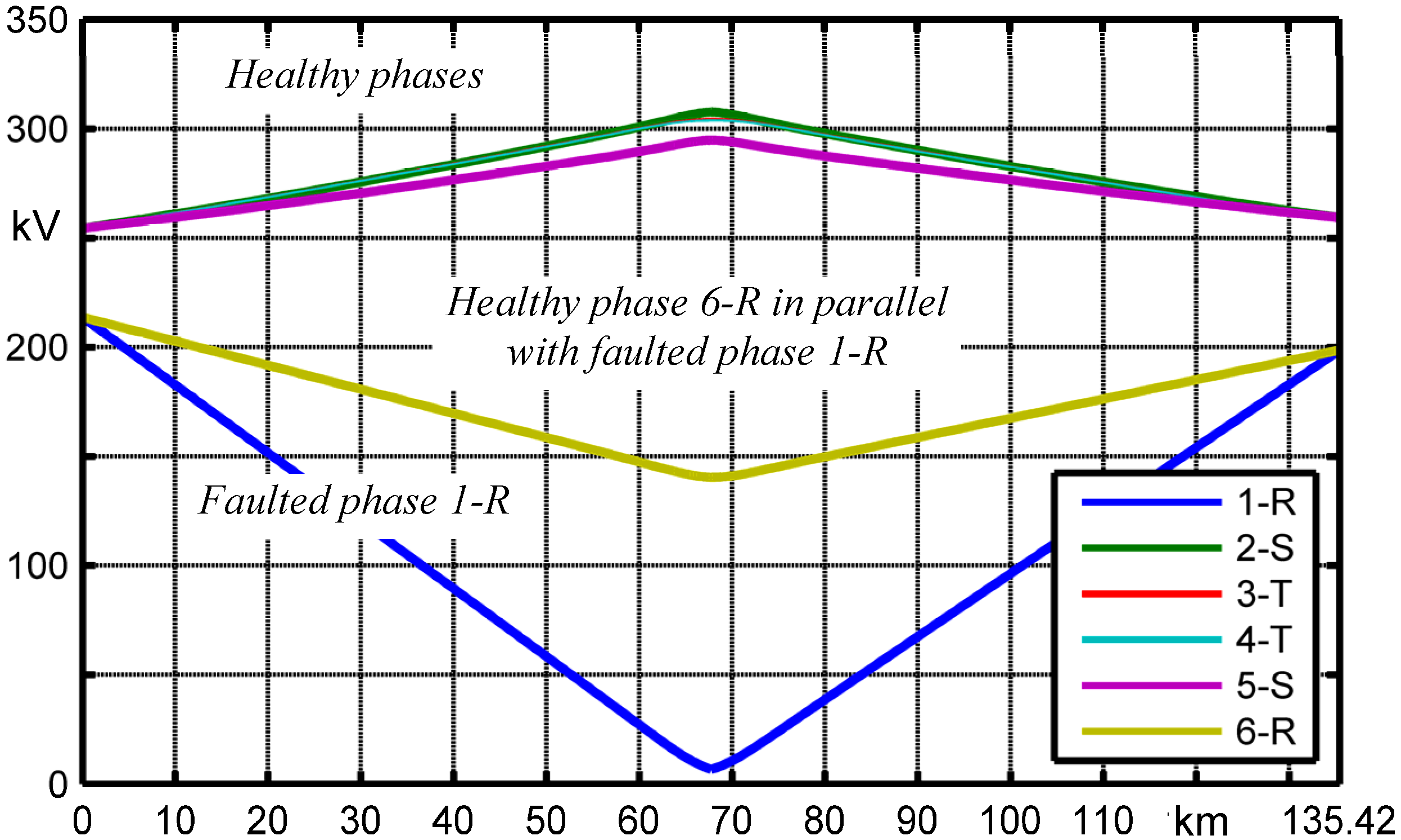
Figure 16 shows the phase voltage magnitudes along the OHL. At midline the phase 1-R voltage magnitude is equal to the tower voltages (which is the same voltage of the earth wire). Also the phase 6-R of healthy circuit has a voltage drop whereas all the other phase voltage magnitudes have an overvoltage. These ones are the so called “temporary overvoltages due to earth faults” or power frequency overvoltages of relatively long duration.

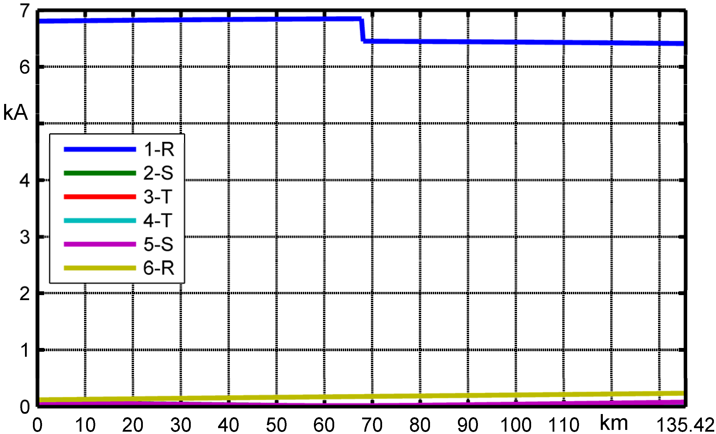
Figure 17 shows the current sharing between the six phases: 6.85 kA coming from substation SEND. and 6.45 kA from substation REC. due to the different fault levels. The fault current |I_1P-1R| is equal to 13.304 kA whereas healthy phases (or un-faulted phases) have almost zero current. Beyond the faulted phase 1-R, the only not-negligible short circuit current flows in the phase which is in parallel with 1-R i.e., 6-R (since “low reactance” phasing has been applied). The short circuit currents in all the other phases are almost zero since, according to IEC 60909-0, the shunt load admittance can be neglected so that the faulted network is at no-load.

Figure 16. Line-to-earth voltage magnitudes along the line.

Figure 16. Line-to-earth voltage magnitudes along the line.

Figure 17. Phase current magnitudes along the line.

Figure 17. Phase current magnitudes along the line.

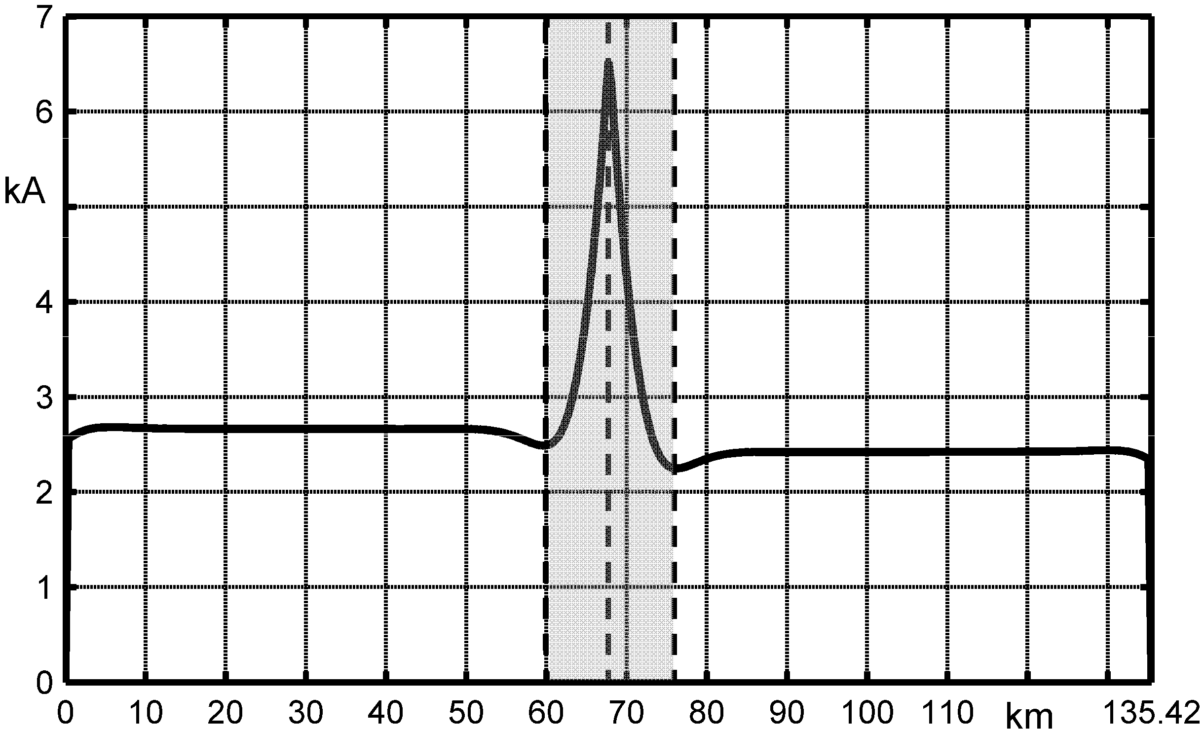
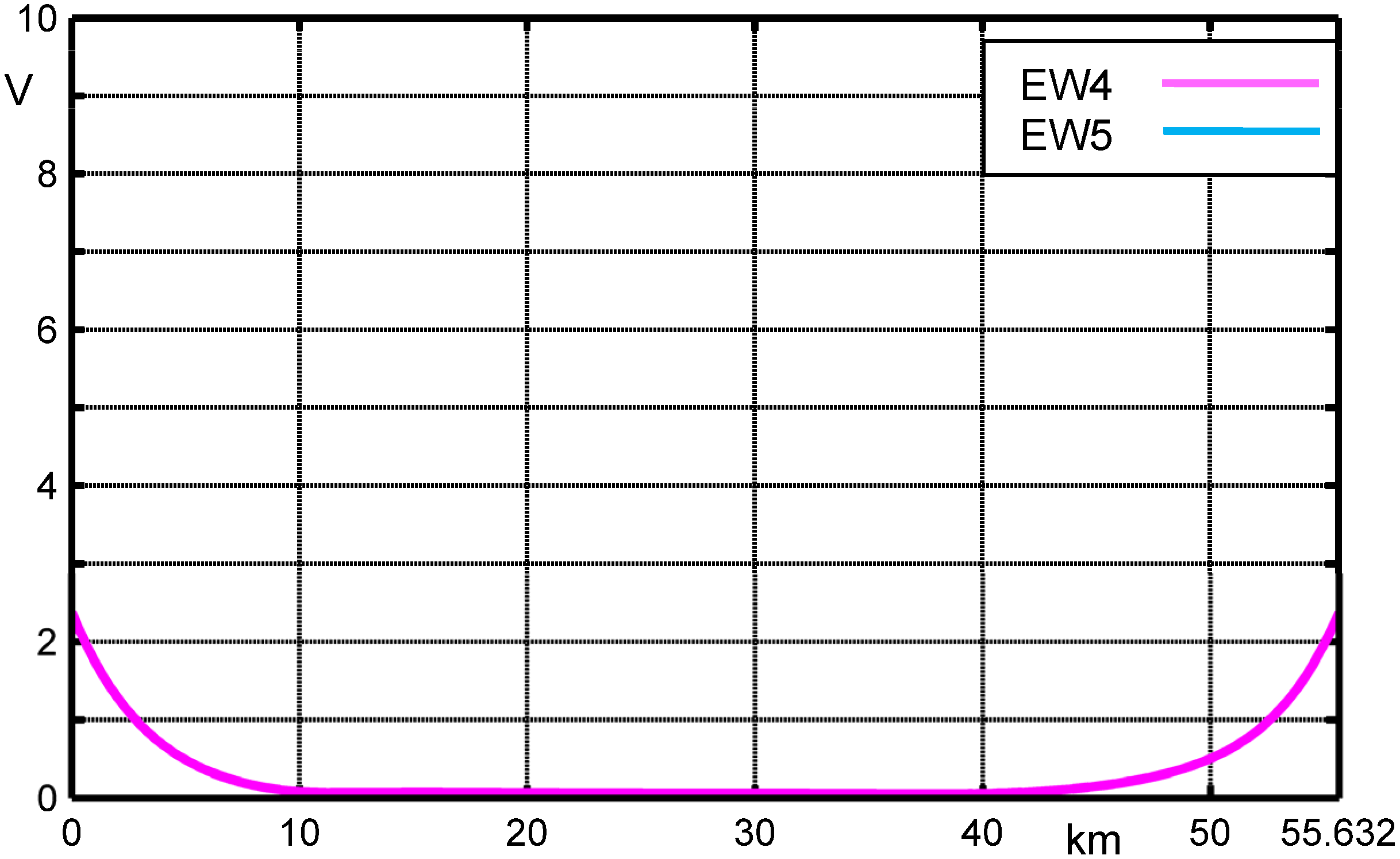
The earth wire current magnitude |I_EW| (see Figure 18) decreases from the fault location up to a given number of spans injecting current into the earth. This number of spans, after which there is not current injection into the earth anymore, can be theoretically evaluated [7,13]. By observing Figure 18 it can be ascertained that after 8 km from the fault location the earth wire stops injecting current into the earth. 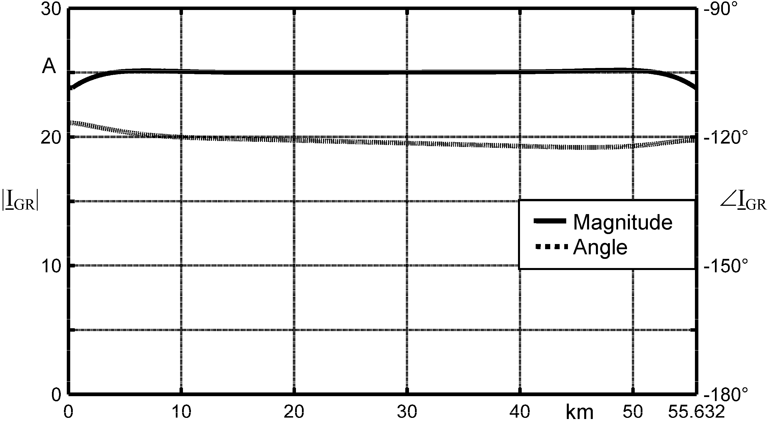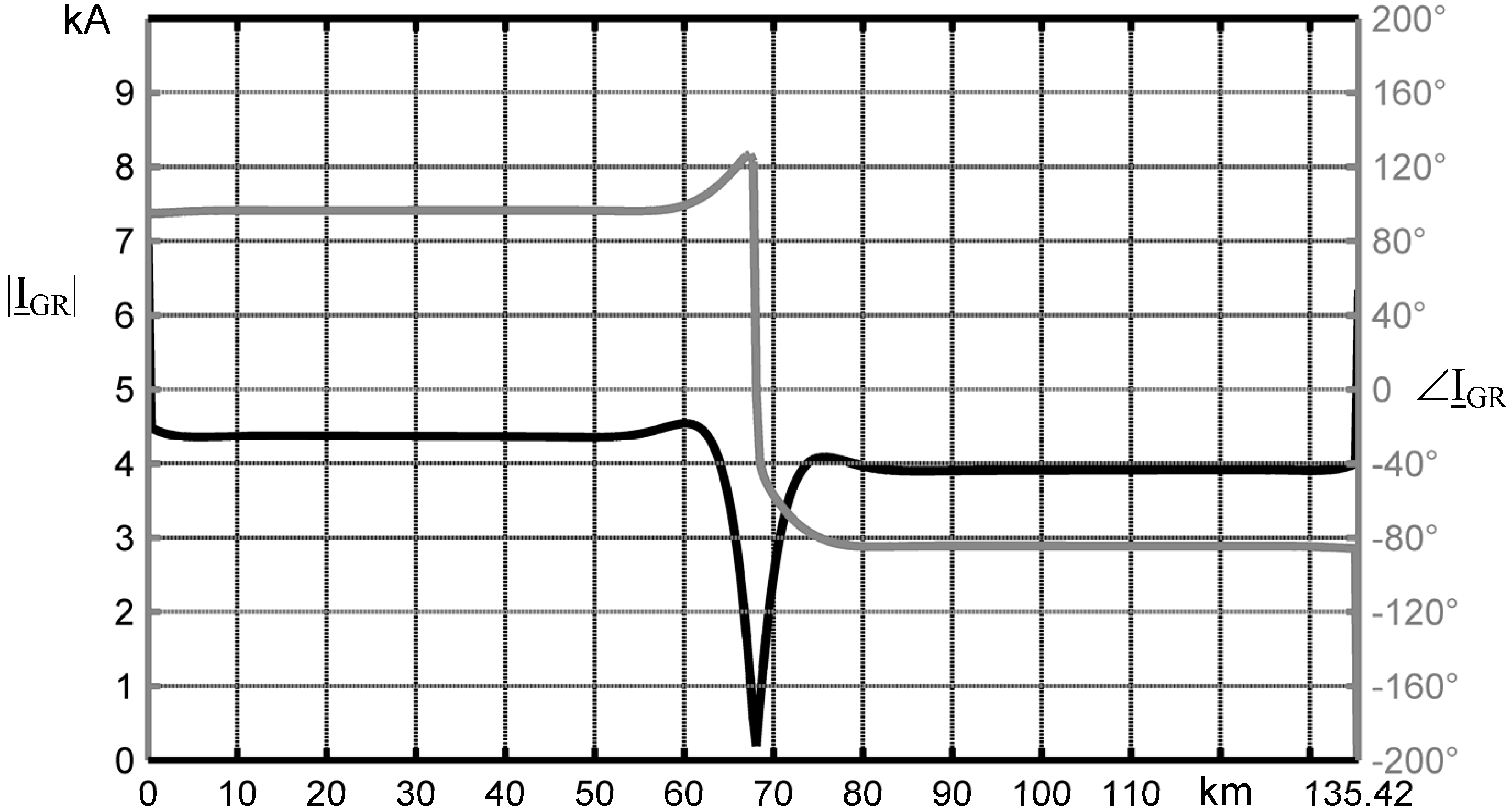Figure 19 shows the ground return current magnitudes and the angles for a midline short-circuit along the line.

It is worth noting that the exact knowledge of the ground return current behaviour results fundamental when evaluations of EMI must be assessed in a given point along the line so that the only knowledge of the sending and receiving end values |I_GR| are not enough.

Figure 18. Earth wire current magnitude |I_EW| along the line in fault condition.

Figure 18. Earth wire current magnitude |I_EW| along the line in fault condition.

Figure 19. Ground return current magnitude |I_GR| and angle along the line in fault condition.

Figure 19. Ground return current magnitude |I_GR| and angle along the line in fault condition.

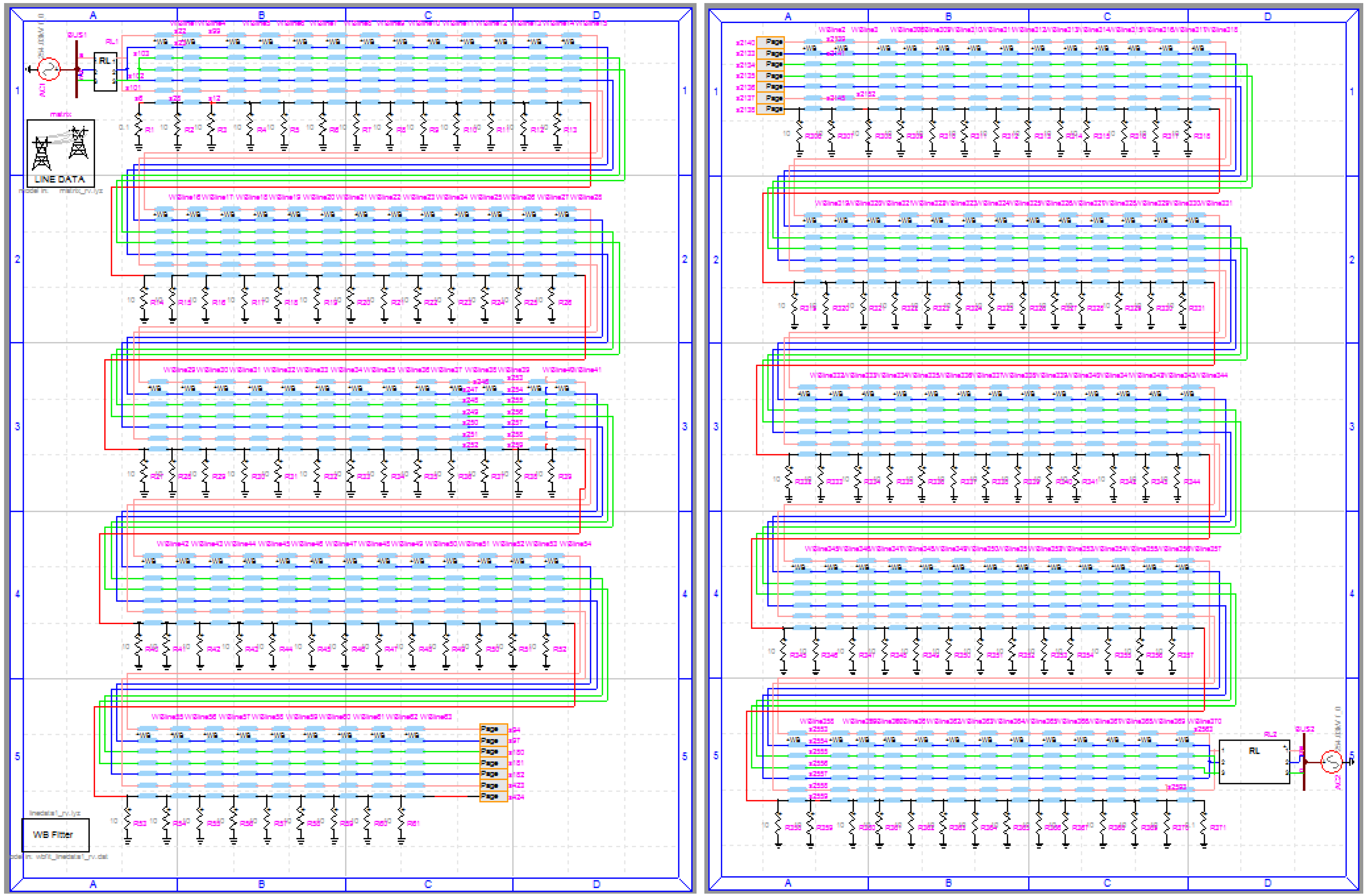
Comparison with EMTP-RV

Some of the above presented MCA results are compared with the EMTP-RV ones for the OHL of previous section whose EMTP-RV electrical layout is shown in Figure 20.

Figure 20. EMTP-RV double-circuit OHL electrical layout (pages 1/6 and 6/6).

Figure 20. EMTP-RV double-circuit OHL electrical layout (pages 1/6 and 6/6).

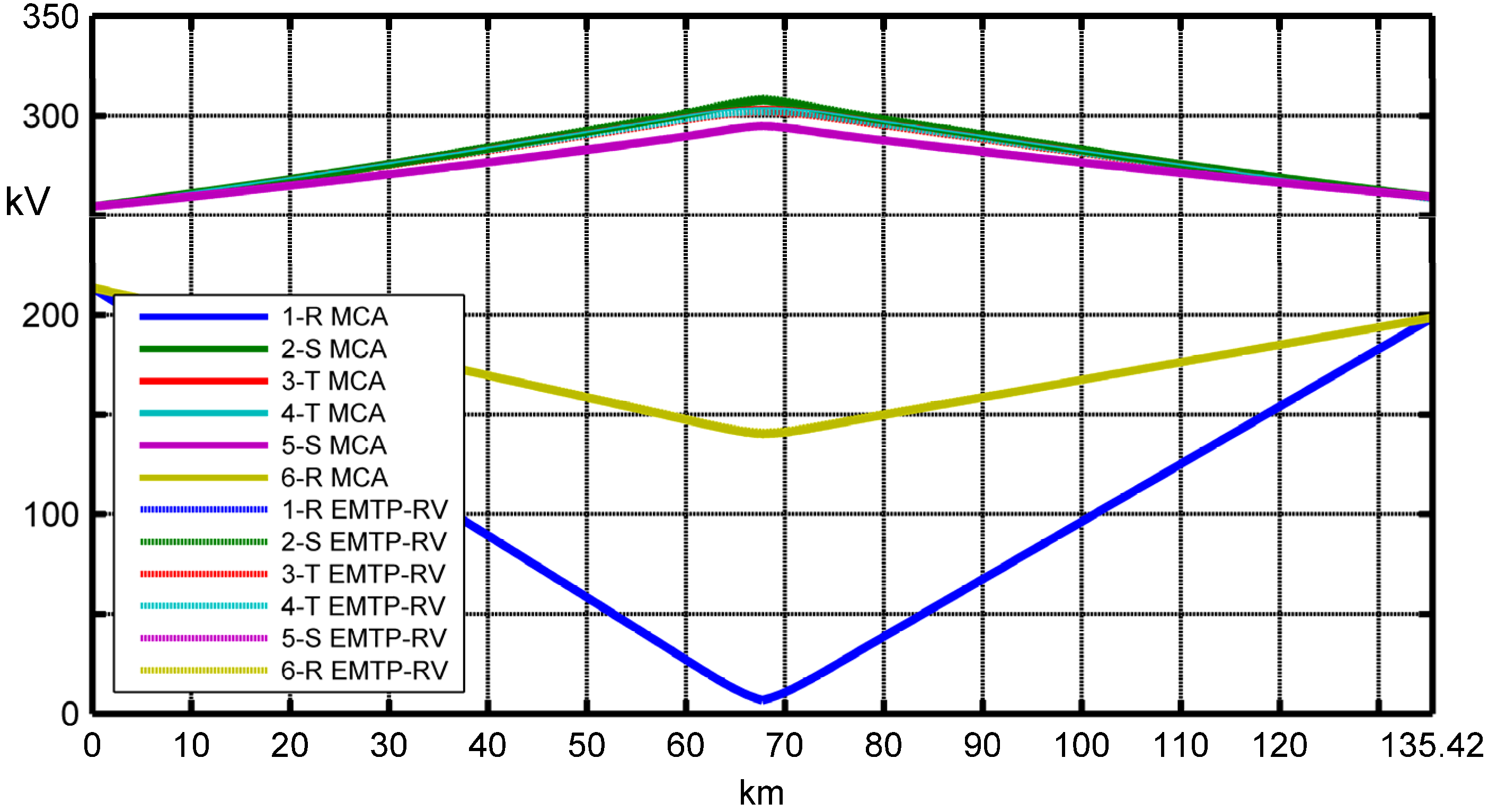
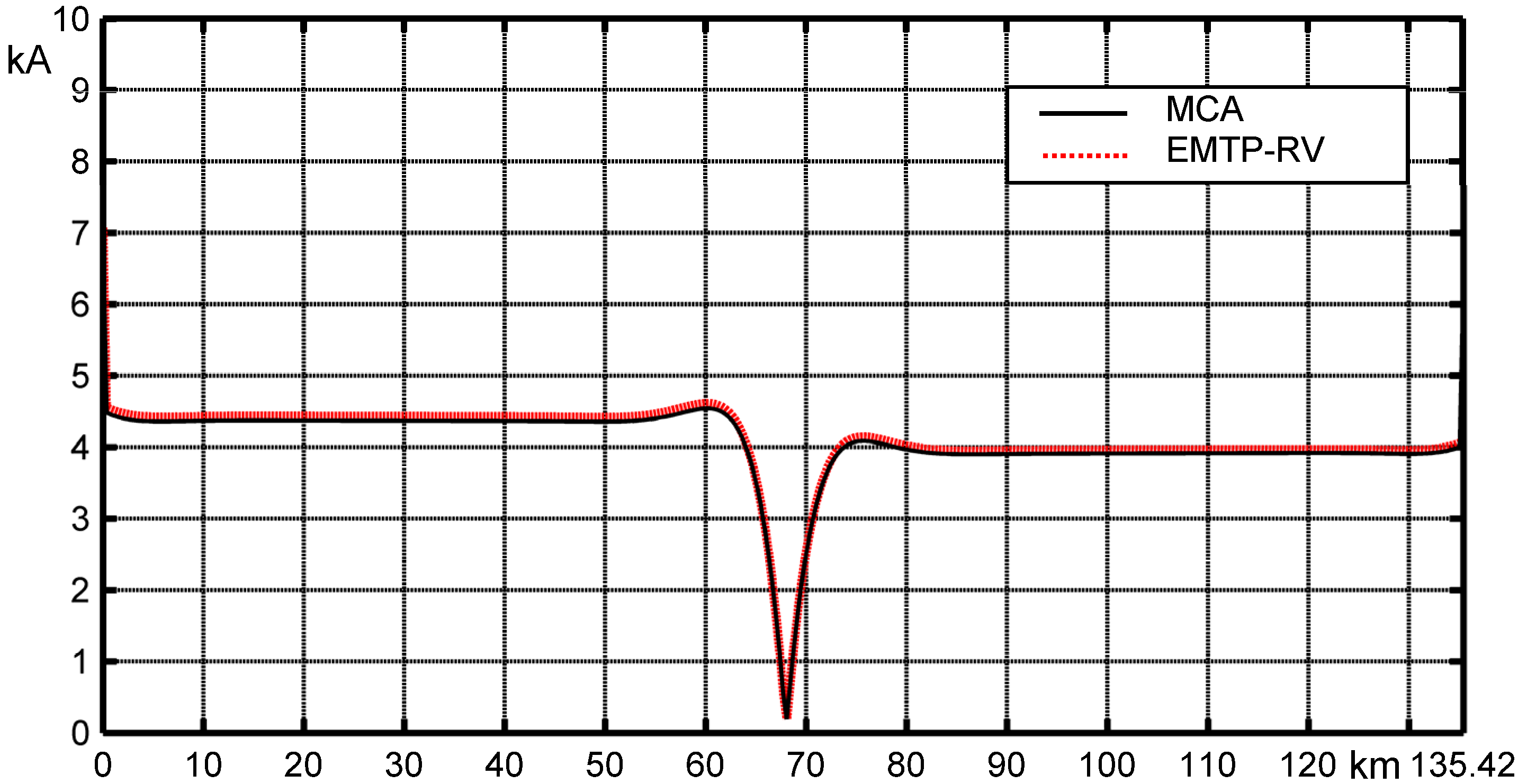
Figure 21 shows the phase voltage magnitude behaviors along the double circuit OHL by means of MCA and EMTP-RV. The maximum percentage voltages for each phase are reported in Table 5 where the maximum value is equal to 0.95%. The cpu-time in the simulation with MCA is 3.41 s and with EMTP-RV is 3.5 s (INTEL CORE 2 QUAD [email protected] GHz, 3.25 GB RAM). |I_GR| comparison is shown in Figure 22. The maximum difference between the MCA and EMTP-RV ground current magnitude is 77 A (−1.9%). In conclusion, the agreement between MCA and EMTP-RV is extremely good.

Figure 21. Line-to-earth voltage magnitude comparison between the MCA and EMTP-RV under phase-to-earth short circuit in a double-circuit OHL.

Figure 21. Line-to-earth voltage magnitude comparison between the MCA and EMTP-RV under phase-to-earth short circuit in a double-circuit OHL.

Table 5. Double-circuit line maximum voltage magnitude comparison.

Eliminate	Max. faulted circuit voltage magnitudes [kV]			Max. healthy circuit voltage magnitudes [kV]
	Phase 1-R (faulted phase)	Phase 2-S	Phase 3-T	Phase 6-R	Phase 5-S	Phase 4-T
MCA	6,68	307,7	304,6	140,4	294,8	303,8
EMTP-RV	6,74	308,8	301,7	141,4	295,3	301,9
Percentage difference	−0.9%	−0.36%	0.95%	−0.71%	0.16%	0.62%

Table 5. Double-circuit line maximum voltage magnitude comparison.

Eliminate	Max. faulted circuit voltage magnitudes [kV]			Max. healthy circuit voltage magnitudes [kV]
	Phase 1-R (faulted phase)	Phase 2-S	Phase 3-T	Phase 6-R	Phase 5-S	Phase 4-T
MCA	6,68	307,7	304,6	140,4	294,8	303,8
EMTP-RV	6,74	308,8	301,7	141,4	295,3	301,9
Percentage difference	−0.9%	−0.36%	0.95%	−0.71%	0.16%	0.62%

Figure 22. Ground return current comparison between the MCA and EMTP-RV under line-to-earth short circuit in a double-circuit OHL.

Figure 22. Ground return current comparison between the MCA and EMTP-RV under line-to-earth short circuit in a double-circuit OHL.

5. Conclusions

MCA has already had a great number of successful applications to multi-phase asymmetrical systems [1,2,3]. In this paper, it has been applied to overhead lines with bundled phase conductors and one or more earth wires. The steady state regime of a typical un-transposed HV OHL has highlighted that there is a not negligible ground return current which may lead to electromagnetic interferences and ac corrosion issues. In faulty analysis, the behaviour of ground return current can be directly achieved so to recognize the number of spans after which the injection of currents in the ground terminates and the ground return current becomes constant. MCA is also extremely useful to evaluate the rise of earth potential at substation sites. Further researches are needed in order to validate the screening factor approach by means of MCA tool. Comparisons with EMTP-RV commercial software has demonstrated a very good agreement.