Decisions on Energy Demand Response Option Contracts in Smart Grids Based on Activity-Based Costing and Stochastic Programming

Abstract
:1. Introduction
- (1)
- USP’s call option offer: USP offers to an industrial customer a call option offer according to a predefined energy demand response program. The option has an option premium price of $20/kW per month and a strike price of $1/kW per hour for actual energy load curtailments. The option allows exercise during the life of the option that is in the months of June through September. The option is constrained to be exercised during peak hours (12 noon to 8 p.m.) of weekdays and up to 20 h per month.
- (2)
- Customer’s acceptance of the offer: The industrial customer agrees to provide 200 kW of load curtailment at any time during the contracted period. The total option premium given to the industrial customer is $16,000 (= 4 months × $20/kW × 200 kW).
- (3)
- USP’s exercise of the option: On a certain day during the contracted period, USP falls into a situation where the overall energy demand increases rapidly and so it needs to exercise the option. USP then commands the industrial customer to curtail 200 kW from 2 p.m. to 6 p.m.
- (4)
- Customer’s load curtailment: According to the contract, the industrial customer reduces 200 kW from its contracted baseline usage rate. The determination if the customer abides by the command is verified through reading of metering devices. If the load curtailment is not achieved, the customer is subject to penalty. If the reduction is made per contract, the customer is paid $800 (= 200 kW × 4 h × $1/kW per hour) that corresponds to the strike price.

| Notation | Description |
|---|---|
| Set of activity (e.g., = {operating robots, moving conveyors, air conditioning, building lighting, …}) where , , and represent sets for mission-critical activities, state-transition flexible activities, and QoS flexible activities, respectively (See Section 3 for details) | |
| Set of state where = {production, shutdown, startup, setback, maintenance} | |
| Set of utility (e.g., = {electricity, natural gas, oil, compressed air, …}) | |
| Rate of energy demand (also called power, kW) of activity at state | |
| Activity state time function; at any given and time (See Section 4 for details) | |
| Time period of energy demand response option exercising defined in an energy demand response option contract (e.g., 2 h starting from noon, which is represented by where and ) | |
| Energy delivery rate (kW) during defined in an energy demand response option contract | |
| Peak rate of energy demand (kW) during where , , and represent the peak rate of energy demands (kW) for activities in , , , respectively for a given time period | |
| Energy load (kWh) during where , , and represent energy demands (kWh) for activities in , , , respectively for a given time period | |
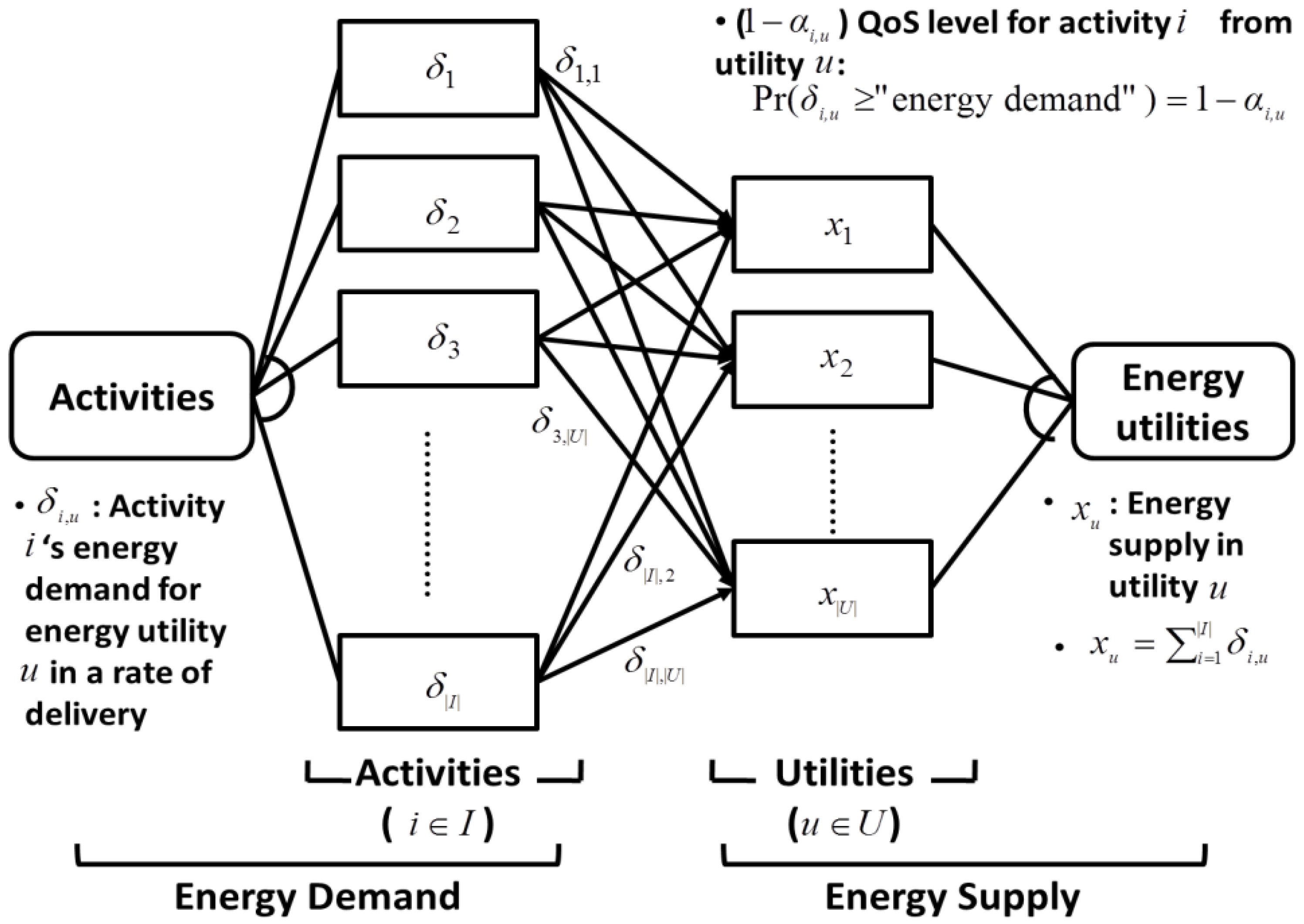
| Energy supply rate (kW) of utility for activity | |
| Energy demand rate (kW) of activity for activity | |
| Probability to fail meet a quality of service (QoS) required to activity that consumes utility . Accordingly, (1-) represents the probability to meet the required level of QoS |
2. Related Works
3. Background Technologies
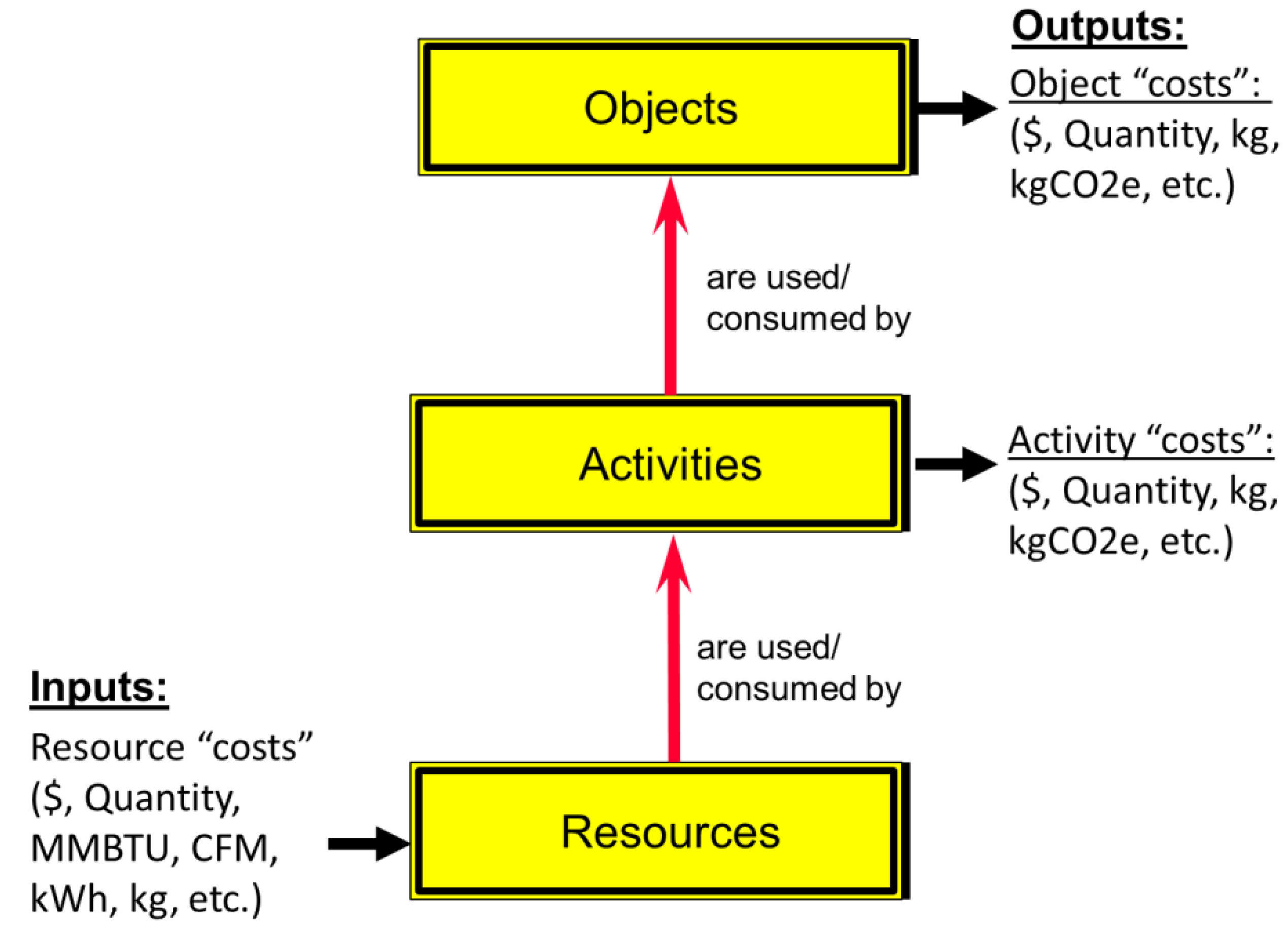
3.1. Activity-Based Costing (ABC)

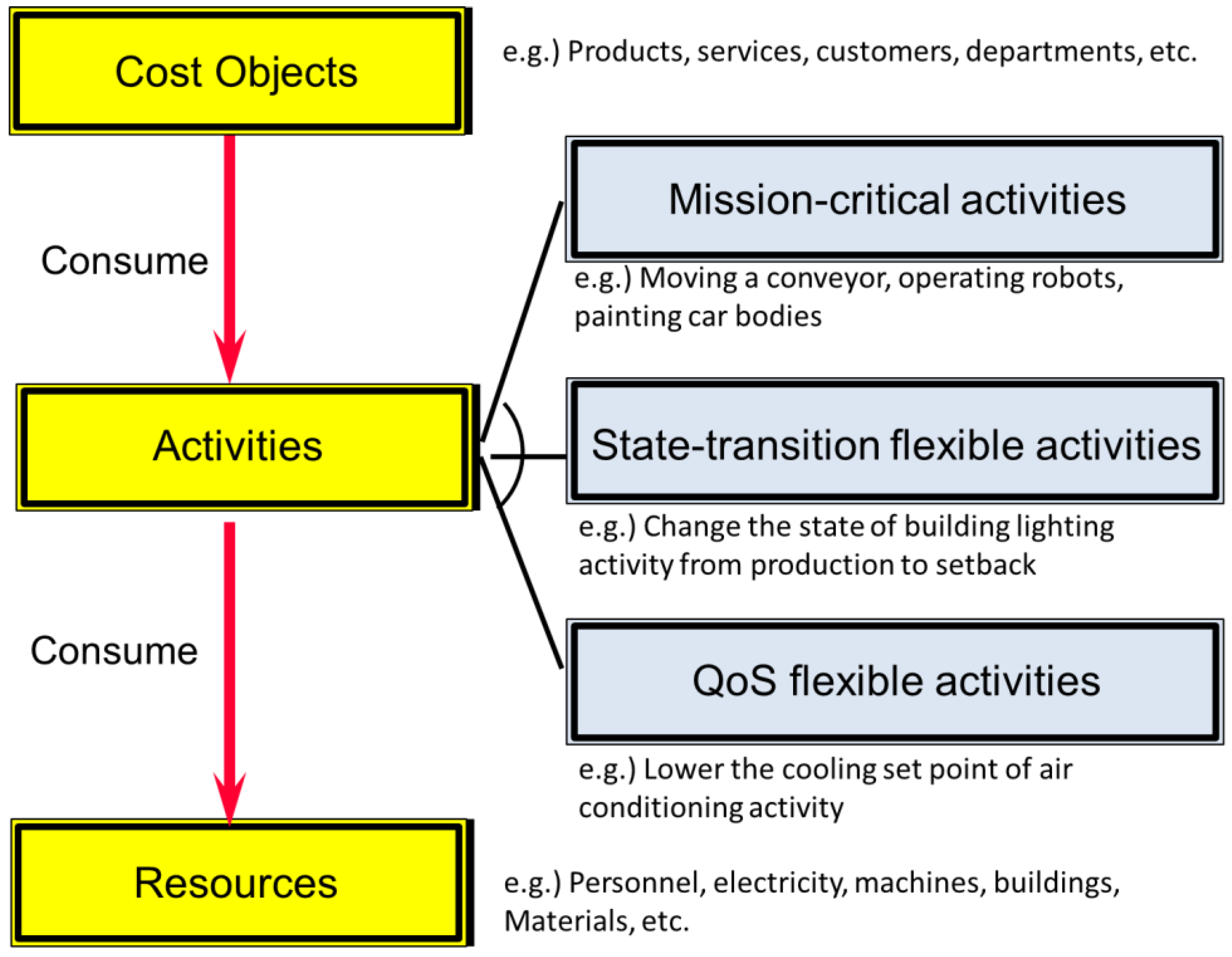
- Definition 1 (Mission critical activity) An activity is mission-critical if the activity’s failure results in the failure of business operations where denotes a set of mission-critical activities.
- Definition 2 (State-transition flexible activity) An activity is state-transition flexible if the activity’s state can transition to any or some of the defined states as a result of energy load-shedding processes where denotes a set of state-transition flexible activities.
- Definition 3 (QoS flexible activity) An activity is QoS flexible if the quality of service (QoS) level imposed on the activity can be adjusted in terms of the probability to meet the QoS where denotes a set of QoS flexible activities.
- Proposition 1 (Flexibility of activities) Any activity is flexible if .
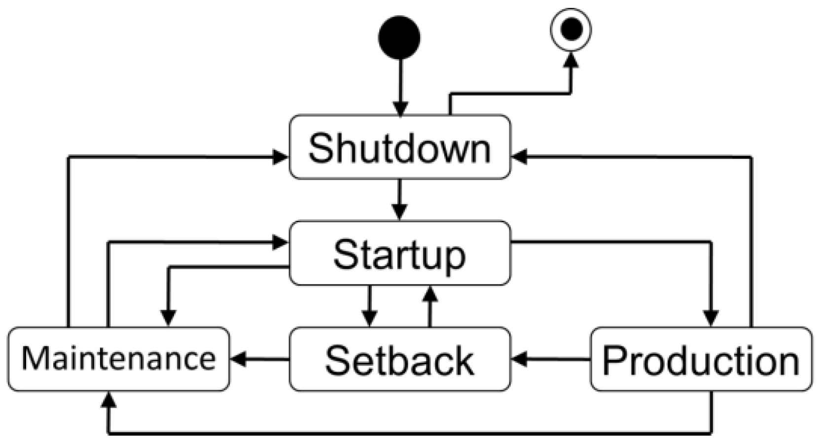
- Production state: It is a state in which products are being produced on the manufacturing system. This state requires a high level of energy due to most equipment in the facility running at high levels when in this state;
- Setback state: It is a state for lunch or between shifts which occur during a normal working days when the system can be put in a ready state to save energy. In this state, the equipment of the system is turned down to a lower level or off until production resumes again;
- Shutdown state: If there is an extended period in which the system does not need to run such as weekends or holidays, the system can be put in the shutdown state, in which the system is turned off and uses minimal energy;
- Startup state: To transfer from the shutdown state to the production state, the system requires a high level of energy and is put into a startup state. This state is a high consumer of energy because the system is operated to quickly increase system conditions to operating conditions. This is similar to the time when a vehicle accelerates, in which it requires more gas than when cruising or parked;
- Maintenance state: During the maintenance state, necessary repairs are performed with minimal energy requirement.
3.2. Stochastic Programming

4. Decision Model for Determining Energy Demand Response Option Contract
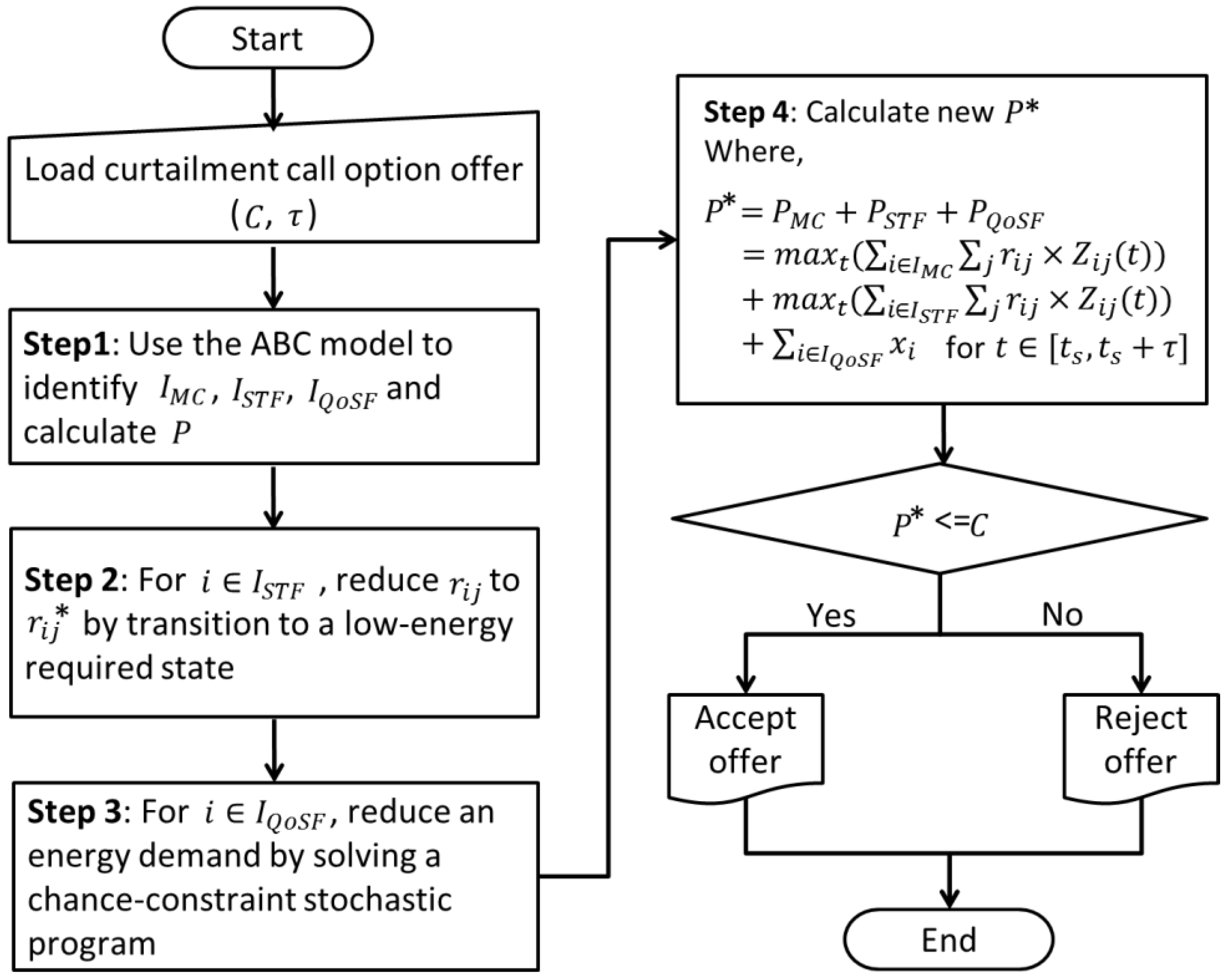
- Step 1: With a new load curtailment offer arrived, use the ABC model and identify ,, and calculate the current peak energy demand rate, . This step requires an ABC-based energy accounting model for manufacturing operations. The basic idea in modeling is that each activity has five distinct states (i.e., production, shutdown, startup, setback, maintenance) and makes transitions from one state to other state according to a production schedule such that an activity is always put in only one state in any given time. The key point is that each state has a different energy load characteristic. And furthermore, the activities listed in the ABC-based energy accounting model are broken down into mission-critical () and non-mission critical activities (,). Again, the operation specifications of non-mission critical activities are given in ranges allowing flexibility of the state transition or QoS adjustment, resulting in a lower energy demand.
- Step 2: Investigate the amount of possible reduction in the energy demand (kW) for each activity by transition to a low-energy required state (i.e., transition to , such that ).
- Step 3: Investigate the amount of possible reduction in the energy demand (kW) for each activity by solving a chance-constraint stochastic problem through varying the QoS level (i.e., reduce such that decreases).
- Step 4: Recalculate the peak energy demand level and denote the new peak energy demand level by and determine whether to accept or reject the offer based on and .

5. Illustrative Example
- = {Manual assembly, Operating robots, Moving conveyors, Operating repairing centers, Air conditioning, Building lighting, Operating chillers, Liquid moving, Air abatement};
- = {production, shutdown, startup, setback, maintenance};
- = {electricity};
- = 2 h with the start time at 12:00 p.m., implying that the time period of energy demand response option exercising is where =12:00 p.m.;
- = 280 kW that is an energy delivery rate (kW) defined in the option contract.
5.1. Identify ,, and Calculate the Current
- = {Manual assembly, Operating robots, Moving conveyors, Operating repairing centers};
- = {Building lighting, Liquid moving, Air abatement};
- = {Air conditioning, Operating chillers};
- The ordinary peak rate of energy demand (kW), (=++) during is assumed to be higher than implying that the company needs to determine as to whether they can reduce their peak energy demand by (.
5.2. Reduction in the Rate of Energy Demand (kW) for State-Transition Flexible Activities
| Activity () | State () | ||||
|---|---|---|---|---|---|
| Startup | Production | Setback | Shutdown | Maintenance | |
| Building lighting | 10 kW | 10 kW | 4 kW | 1 kW | 4 kW |
| Liquid moving | 55 kW | 20 kW | 10 kW | 0 kW | 0 kW |
| Air abatement | 30 kW | 10 kW | 2 kW | 0 kW | 0 kW |
5.3. Reduction in the Rate of Energy Demand (kW) for QoS Flexible Activities
| Demand | |||||
|---|---|---|---|---|---|
| 2 kW s.t. | 3 kW s.t. | 4 kW s.t. | 5 kW s.t. | 6 kW s.t. | |
| = 0.65 | = 0.1 | = 0.1 | = 0.1 | = 0.05 | |
| 20kW s.t. | 40kW s.t. | 60kW s.t. | 80kW s.t. | 100kW s.t. | |
| = 0.7 | = 0.15 | = 0.1 | = 0.04 | = 0.01 |
5.3.1. Objective Function, Variables, and Parameters
| Variables | Definition |
|---|---|
| Total demand in electricity load | |
| Variables corresponding to the stochastic electricity demand for air conditioning | |
| 1 if k-th demand (air conditioning) is satisfied in the K-bin discretized demand distribution, otherwise 0 | |
| Variables corresponding to the stochastic electricity demand for air conditioning | |
| 1 if k-th demand (operating chillers) is satisfied in the K-bin discretized demand distribution, otherwise 0 |
| Variables | Definition |
|---|---|
| Electricity demand for manual assembly (6 kW) | |
| Electricity demand for operating robots (8 kW) | |
| Electricity demand for moving conveyors (163 kW) | |
| Electricity demand for operating repairing centers (17 kW) | |
| Stochastic electricity demand for air conditioning as specified in Table 3 | |
| Electricity demand for building lighting at Setback state (4 kW) | |
| Stochastic electricity demand for operating chillers as specified in Table 3 | |
| Electricity demand for liquid moving at Setback state (10 kW) | |
| Electricity demand for air abatement at Setback state (2 kW) | |
| Probability to fail in meeting a quality of service (QoS) required for the air conditioning activity | |
| Probability to fail in meeting a quality of service (QoS) required for the operating chillers activity |
5.3.2. Constraints
5.3.3. Results
5.4. Calculate a New Peak Energy Demand () and Make a Decision on the Offer
6. Conclusions
References
- Electric Power Research Institute (EPRI). Report to NIST on Smart Grid Interoperability Standards Roadmap; Contract No. SB1341-09-CN-0031-Deliverable 10. Available online: http://www.nist.gov/smartgrid/upload/Report_to_NIST_August10_2.pdf (assessed on 9 August 2012).
- Cazalet, E.G. Transactional energy market information exchange (TeMIX). An OASIS Energy Market Information Exchange Technical Committee White Paper. Available online: http://www.cazalet.com/images/Transactional_Energy_CW_2010_Cazalet.pdf (assessed on 9 August 2012).
- Kolta, T. Selecting Equipment to Control Air Pollution from Automotive Painting Operations; SAE Technical Paper 920189; International Congress & Exposition: Detroit, MI, USA, 1992. [Google Scholar]
- Streitberger, H.-J.; Dössel, K.-F. Automotive Paints and Coatings; Wiley: Weinheim, Germany, 2008. [Google Scholar]
- Emblemsvag, J.; Bras, B. Activity-Based Cost and Environmental Management: A Different Approach to ISO 14000 Compliance; Kluwer Academic: Boston, NY, USA, 2001. [Google Scholar]
- Romaniw, Y.; Bras, B.; Guldbert, T. An activity based approach to sustainability assessments. In Proceedings of American Society of Mechanical Engineers (ASME) 2009 Int’l Design Engineering Technical Conferences & Computers and Information in Engineering Conference (IDETC/CIE 2009), San Diego, CA, USA, 30 August–2 September 2009.
- Vlasic, B. With sonic, G.M. stands automaking on its head. The New York Times. 12 July 2011. Available online: http://www.nytimes.com/2011/07/13/business/with-chevrolet-sonic-gm-and-uaw-reinvent-automaking.html (assessed on 9 August 2012).
- Yoo, J.; Park, B.; An, K.; Al-Ammar, E.A.; Khan, Y.; Hur, K.; Kim, J.-H. Look-ahead energy management of a grid-connected residential PV system with energy storage under time-based rate programs. Energies 2012, 5, 1116–1134. [Google Scholar] [CrossRef]
- Soares, J.; Canizes, B.; Lobo, C.; Vale, Z.; Morais, H. Electric vehicle scenario simulator tool for smart grid operators. Energies 2012, 5, 1881–1899. [Google Scholar] [CrossRef]
- Ghatikar, G.; Piette, M.A.; Fujita, S.; McKane, A.; Dudley, J.H.; Radspieler, A.; Mares, K.C.; Shroyer, D. Demand Response and Open Automated Demand Response Opportunities for Data Centers; Lawrence Berkeley National Laboratory: Berkeley, CA, USA, 2010. Available online: http://drrc.lbl.gov/publications/demand-response-and-open-automated-demand-response-opportunities-data-centers (assessed on 9 August 2012).
- Jurek, P.; Bras, B.; Guldberg, T.; D’Arcy, J.B.; Oh, S.-C.; Biller, S.R. ABC applied to automotive manufacturing. In Proceedings of IEEE Power & Energy Society General Meeting, San Diego, CA, USA, 22–26 July 2012.
- Popesko, B. Activity-based costing application methodology for manufacturing industries. E+M Ekonomie Manag. 2010, 13, 103–113. [Google Scholar]
- Moolman, A.J.; Koen, K.; Wethuizen, J. Activity-based costing for vehicle routing problems. S. Afr. J. Ind. Eng. 2010, 21, 161–171. [Google Scholar]
- Sirikitputtisak, T.; Mirzaesmaeeli, P.L. A multi-period optimization model for energy planning with CO2 emission considerations. Energy Proced. 2009, 1, 4339–4346. [Google Scholar] [CrossRef]
- Charnes, A.; Cooper, W.W. Deterministic equivalents for optimizing and satisficing under chance constraints. Operat. Res. 1963, 11, 18–39. [Google Scholar] [CrossRef]
- Sen, S.; Higle, J.L. An introductory tutorial on stochastic linear programming models. Interfaces 1999, 29, 33–61. [Google Scholar] [CrossRef]
- Luedtke, J.; Ahmed, S.; Nemhauser, G. An integer programming approach for linear programs with probabilistic constraints. In Proceedings of the Twelfth Conference on Integer Programming and Combinatorial Optimization (IPCO 2007); Fischetti, M., Williamson, D., Eds.; Springer-Verlag: HBerlin, Germany, 2007; Volume 3, pp. 410–423. [Google Scholar]
- Oh, S.-C.; D’Arcy, J.B.; Arinez, J.F.; Biller, S.R.; Hidreth, A.J. Assessment of energy demand response options in smart grid utilizing the stochastic programming approach. In Proceedings of IEEE Power & Energy Society General Meeting, Detroit, MI, USA, 24–28 July 2011.
- Weil, R.L.; Maher, M.W. Handbook of Cost Management; Wiley: Hoboken, NJ, USA, 2005. [Google Scholar]
- Cokins, G. Activity-Based Cost Management: An Executive’s Guide; John Wiley & Sons: Hoboken, NJ, USA, 2001. [Google Scholar]
- Cox, W.T.; Considine, T. Price Communication, Product Definition, and Service-Oriented Energy; Grid-Interop: Denver, CO, USA, 17–19 November 2009. [Google Scholar]
© 2013 by the authors; licensee MDPI, Basel, Switzerland. This article is an open access article distributed under the terms and conditions of the Creative Commons Attribution license (http://creativecommons.org/licenses/by/3.0/).
Share and Cite
Oh, S.-C.; Hildreth, A.J. Decisions on Energy Demand Response Option Contracts in Smart Grids Based on Activity-Based Costing and Stochastic Programming. Energies 2013, 6, 425-443. https://doi.org/10.3390/en6010425
Oh S-C, Hildreth AJ. Decisions on Energy Demand Response Option Contracts in Smart Grids Based on Activity-Based Costing and Stochastic Programming. Energies. 2013; 6(1):425-443. https://doi.org/10.3390/en6010425
Chicago/Turabian StyleOh, Seog-Chan, and Alfred J. Hildreth. 2013. "Decisions on Energy Demand Response Option Contracts in Smart Grids Based on Activity-Based Costing and Stochastic Programming" Energies 6, no. 1: 425-443. https://doi.org/10.3390/en6010425