1. Introduction
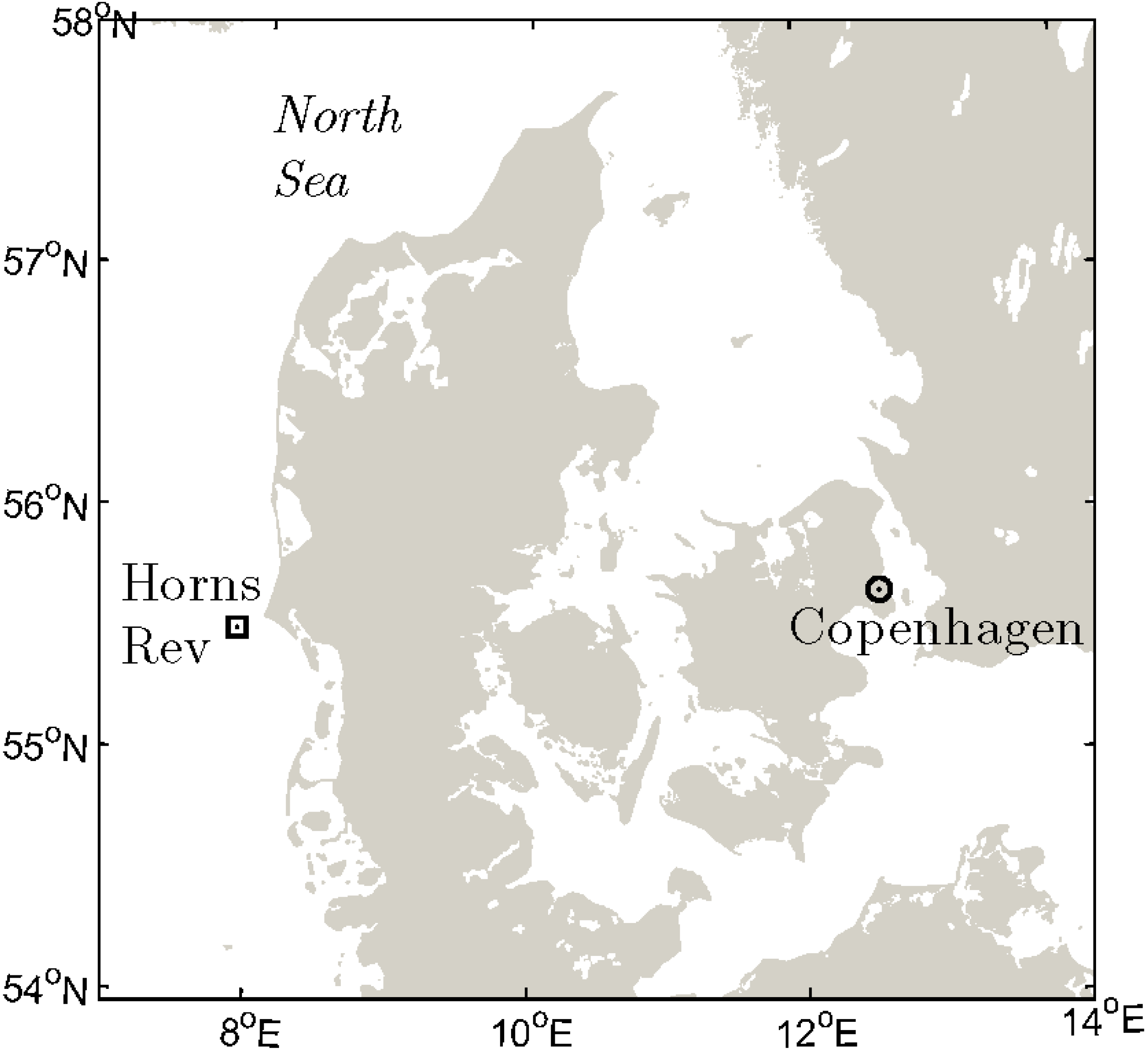
The Horns Rev 1 wind farm is located in the North Sea at about 14 to 20 km offshore from the Danish coastline (
Figure 1).
Figure 1.
Location of the Horns Rev 1 wind farm in the North Sea.
Figure 1.
Location of the Horns Rev 1 wind farm in the North Sea.
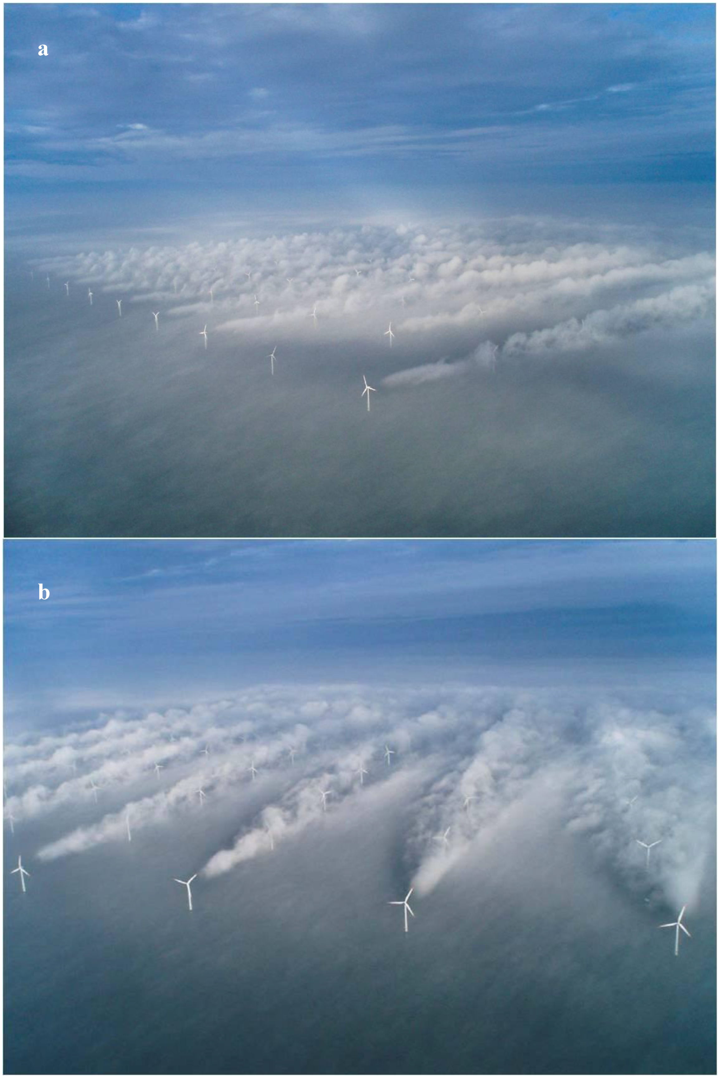
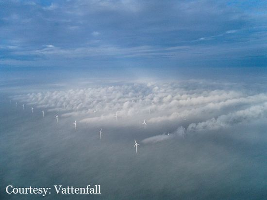
The wake photographs taken at the offshore wind farm at Horns Rev 1 are well known in the wind energy community. They illustrate the wind turbine shadow effect in an attractive manner. The two photographs were taken by the pilot from the window of the helicopter on its way out to the oil rigs in the North Sea at an altitude around 1 to 3 km on 12 February 2008 at around 10:10 UTC. The first photo [
Figure 2(a)] was taken from the southeast and the second [
Figure 2(b)] from the south.
The aim of the paper is to examine the case from combined satellite data, local meteorological observations, radio-sounding data and Supervisory Control and Data Acquisition (SCADA) data from the wind farm. The weather conditions are described and an interpretation of the origin of the fog is provided. Furthermore advanced wake modeling with Computational Fluid Dynamics (CFD) using Detached Eddy Simulation (DES) of a full wind turbine rotor is included to detail the physical processes in the wake of the wind turbines in relation to the formation and dispersion of fog. The meteorological observations, the operation of the wind turbines and the mechanically-driven convection are discussed.
Figure 2.
(a) Upper panel: Photograph of the Horns Rev 1 offshore wind farm 12 February 2008 at around 10:10 UTC seen from the southeast. (b) Lower panel: Same as (a) but shortly after, seen from the south. Courtesy: Vattenfall. Photographer is Christian Steiness.
Figure 2.
(a) Upper panel: Photograph of the Horns Rev 1 offshore wind farm 12 February 2008 at around 10:10 UTC seen from the southeast. (b) Lower panel: Same as (a) but shortly after, seen from the south. Courtesy: Vattenfall. Photographer is Christian Steiness.
3. Data from Satellites and Weather Conditions
3.1. Satellite Maps
Earth observation satellites provide images of the atmospheric and oceanographic conditions. Satellite maps of the clouds, ocean winds and sea surface temperatures are presented and described to detail the met-ocean conditions on the specific morning.
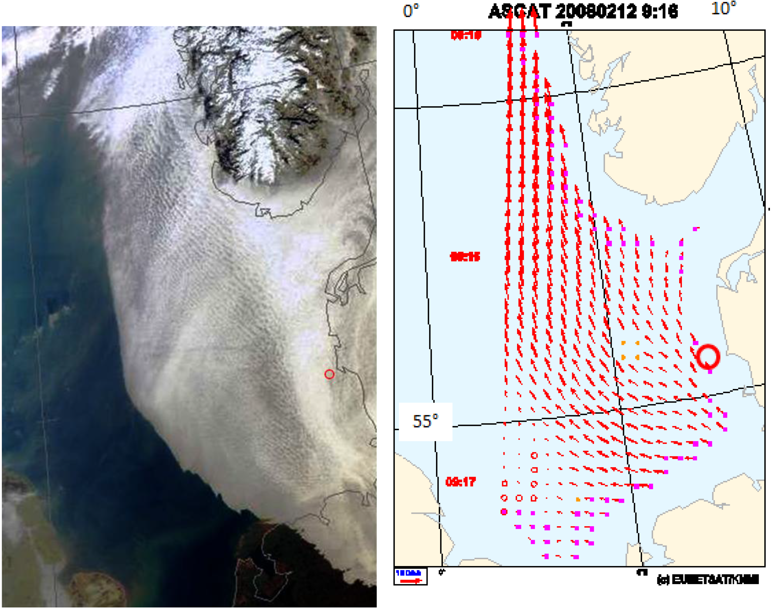
On-board the Terra satellite belonging to National Aeronautics and Space Administration (NASA) is the instrument MODIS, the Moderate Resolution Imaging Spectroradiometer with 36 channels from visual to thermal infrared. On 12 February 2008 Terra mapped the North Sea at 10:07 UTC [
Figure 3(a)].
Three other satellites confirm the cloud cover in the wind farm area in the late morning. These include NOAA AVHRR (National Ocean and Atmosphere Administration, Advanced Very High Resolution Radiometer) at 11:43 UTC and Aqua MODIS at 11:50 UTC. The geostationary satellite Meteosat belonging to EUMETSAT (European Organisation for the Exploitation of Meteorological Satellites) shows cloud cover at 12:00 UTC. At 12:00 UTC, low, homogeneous, stratiform clouds covered Horns Rev. Due to the low viewing angle of Meteosat a rather thick appearance of clouds prevails while the NOAA AVHRR and MODIS images taken at a steeper angle reveal a more variable cloud structure. The latter may explain that the wind farm is sunlit in the photos.
The Advanced Scatterometer ASCAT belonging to EUMETSAT observes ocean winds and direction. On the 12 February 2008 at 09:16 UTC ocean surface wind vectors near Horns Rev were from the south ~5 ms
−1 [
Figure 3(b)]. ASCAT was in the descending mode. At 20:45 UTC ASCAT in ascending mode observed similar wind conditions. The QuikSCAT satellite with the SeaWinds scatterometer on-board belongs to NASA. QuikSCAT observed ocean wind speed and wind direction at 05:00 UTC with weak winds around 3 to 5 ms
−1 from the south near Horns Rev. The QuikSCAT evening wind map from 18:54 UTC showed similar wind conditions (see [
4]). QuikSCAT and ASCAT are based on active microwave radar scatterometry, thus the mapping of ocean wind vectors is done day and night and in cloudy conditions.
Figure 3.
(
a) Left panel: Cloud cover over the North Sea observed from MODIS Terra on 12 February 2008 at 10:07 UTC from NERC Satellite Receiving Station, Dundee University, Scotland at
www.sat.dundee.ac.uk. (
b) Right panel: Ocean surface vector winds observed from ASCAT at 12 February 2008 at 09:16 UTC. The map is produced by the EUMETSAT OSI SAF. The red circles indicate the location of the Horns Rev 1 wind farm. The arrow shows 10 ms
−1.
Despite the cloud cover [
Figure 3(a)], the ocean surface vector winds are retrieved [
Figure 3(b)]. The observations from QuikSCAT and ASCAT are both valid at 10 m above sea level and compare well with observations from a meteorological mast near the Horns Rev 1 wind farm. The meteorological mast M6 is located closer to land than the scatterometers cover. Please refer to
section 3.3 for further details on the local observations.
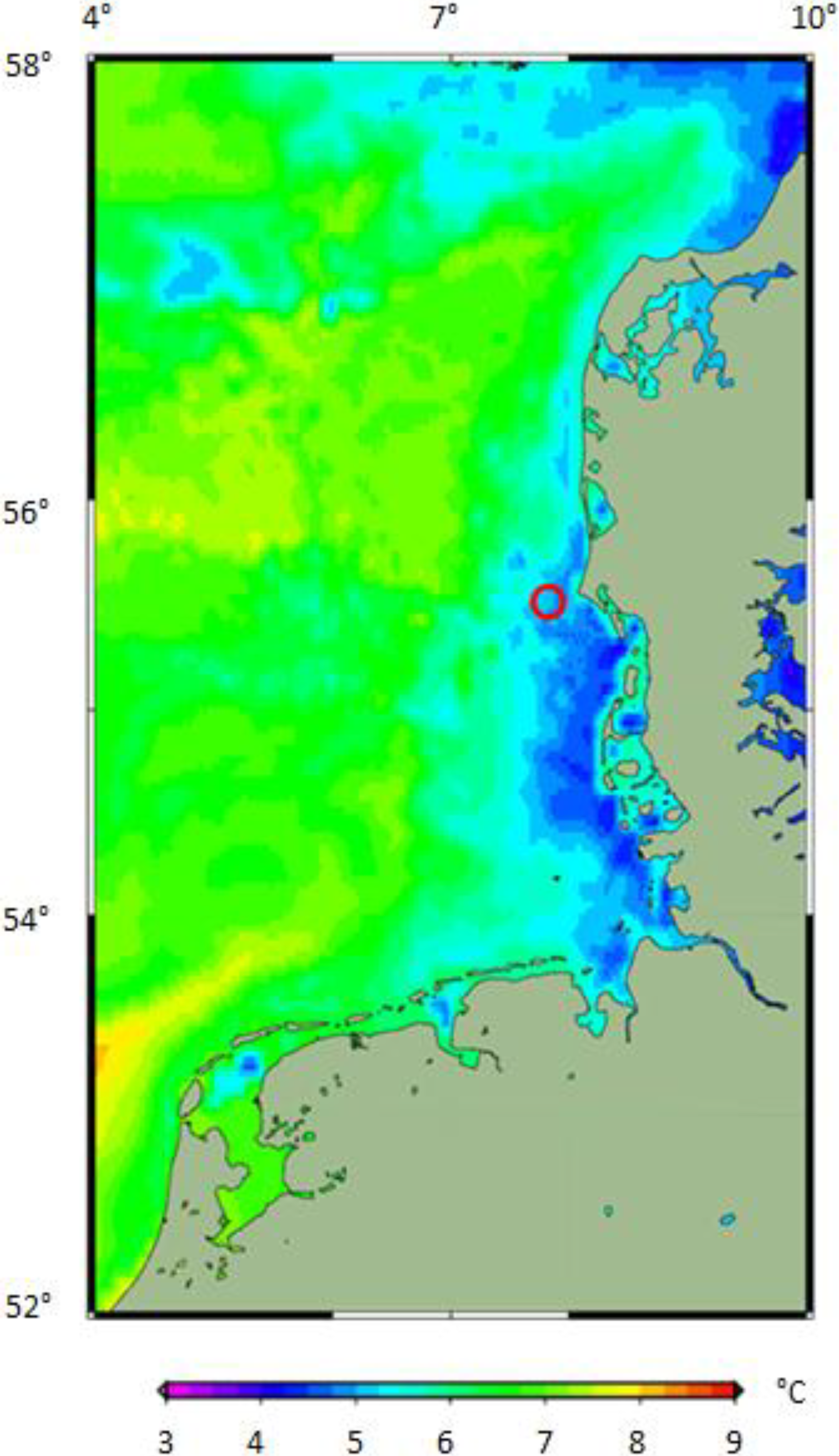
Sea surface temperature (SST) gridded maps are compiled every day from nighttime observations from several satellite instruments.
Figure 4 shows SST of the eastern part of the North Sea from 12 February 2008 at 00:00 UTC.
Figure 4.
Sea surface temperature of the North Sea on 12 February 2008 at 00:00 UTC based on satellite data. The location of the Horns Rev 1 wind farm is indicated with a red circle. Courtesy: Jacob L. Høyer, Danish Meteorological Institute.
Figure 4.
Sea surface temperature of the North Sea on 12 February 2008 at 00:00 UTC based on satellite data. The location of the Horns Rev 1 wind farm is indicated with a red circle. Courtesy: Jacob L. Høyer, Danish Meteorological Institute.
The map is based on a combination of thermal infrared data from the Advanced Along-Tracking Scanning Radiometer (AATSR) on-board the Envisat European Space Agency (ESA) research satellite, NOAA AVHRR, MODIS on-board the Terra and Aqua satellites, and Spinning Enhanced Visible and Infrared Imager (SEVIRI) on-board Meteosat. The advantage of the thermal infrared SST observations is the high spatial resolution while the major disadvantage is that cloud cover limits SST retrievals. Therefore, also passive microwave thermal data are used from the Advanced Microwave Scanning Radiometer (AMSR-E) on-board Aqua. The microwave data are observed in all weather conditions and the spatial resolution is rather coarse, yet blended with the optical data through an objective analysis method that uses statistics to fill out the gaps in time and space producing a higher resolution product. Maps of calculated SST at around 3 km × 3 km spatial resolution and with an error below 0.3 °C in cloud free areas and up to around 0.7 °C in cloud covered areas are obtained every day [
5].
The gridded SST map shows temperatures around 5 °C near Horns Rev. This compares well with the calculated sea temperature of the upper model layer of the Danish Meteorological Institute (DMI) regional three-dimensional ocean model representing 4 m depth. According to the DMI ocean model [
6] and the satellite-based SST map, the water was colder near coast but in general the sea was warmer than the overlying air. The SST observations and ocean model results further compare very well to an observation of sea temperature of 4.7 °C at 3 m depth at the meteorological masts near the wind farm. The masts were operated by DONG energy and Vattenfall. There is a list of data in the
Appendix.
3.2. Weather Conditions
The weather condition in the morning of 12 February 2008 was characterized by very high pressure in Eastern Europe that had spread towards southern Scandinavia resulting in a separate high pressure centre around 1040 hPa in eastern Denmark. This pattern caused light winds to blow from south (S) and southeast (SE) in the wind farm area. Subsidence in the high pressure area formed a temperature inversion, which, however, was at the same time characterized as a frontal inversion as a shallow cold front arrived from northeast (NE) the previous day. The air mass behind the front was of maritime origin, advected from the Norwegian Sea along the northern edge of the high pressure area. Crossing Norway and Sweden on its way to Denmark and the continent it maintained its maritime properties, and cooling from the surface made its humidity condense to widespread fog or low stratus cloud below the inversion [
Figure 3(a)]. Clouds or fog reveal clearly the propagation of a cold and moist air mass.
Just west of Horns Rev the cloudiness looks dense in
Figure 3(a), in agreement with the photos in
Figure 2. In the latter it is possible to distinguish stratiform clouds in the distance. Further west and even around and east of the wind farm warming from below has made the air mass break up into a cellular pattern revealing a vertical mixing process with a partly change of the lapse rate from a wet adiabatic to a dry or near dry adiabatic rate [
Figure 3(a)]. The cellular pattern implies that the clouds dissolve locally, including in the wind farm area. However, the air mass below the inversion stays rather moist. Therefore sea smoke develops over the warm sea surface (
Figure 2), and clouds are restored in its upper part. The fog formation at the wind farm is not distinguishable in the MODIS image [
Figure 3(a)].
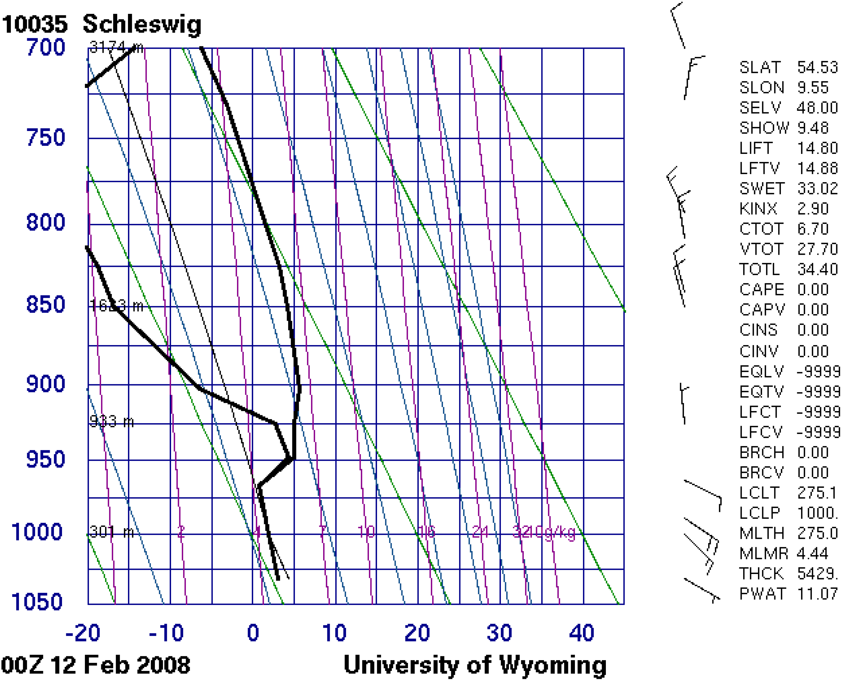
With prevailing winds from the south and southeast, the radio-sounding in Schleswig in northern Germany around 150 km to the SE of the wind farm is assumed to be fairly representative of the air mass over Horns Rev. The soundings reveal a surface inversion on 11 February at 00:00 UTC gradually lifting to a frontal inversion (cf. the change of wind direction with height implying cold air advection). The inversion lifted from around 300 m height at 12.00 UTC on 11 February to 600 m at 00:00 UTC 12 February and to 750 m at 12:00 UTC [
7]. The sounding from 12 February at 00:00 UTC is shown in
Figure 5.
The air was saturated (i.e., with solid cloud) and the lapse rate stable or wet-adiabatic governed below the inversion becoming dry-adiabatic during the day. Dry and warmer air aloft reflects subsidence within the anticyclone.
Figure 5.
Radiosounding data from Schleswig from 12 February 2008 at 00:00 UTC. From [
7].
Figure 5.
Radiosounding data from Schleswig from 12 February 2008 at 00:00 UTC. From [
7].
Increasing cloud thickness at two meteorological stations located east (E) and south-southeast (SSE) of Horns Rev, respectively, Esbjerg Airport 43 km to the E [
8] and List 65 km to the SSE [
9], is thought to be the reason for slightly increasing surface temperatures. At both stations the air temperature increased from around 2 °C to 4 °C from the previous day to 12 February associated with continuous fog or a very low cloud base and periods with drizzle.
3.3. Meteorological Conditions Observed at the Offshore Meteorological Masts
Near the Horns Rev 1 wind farm the local meteorological conditions were observed at two meteorological masts M6 and M7 (see the location of M6 in
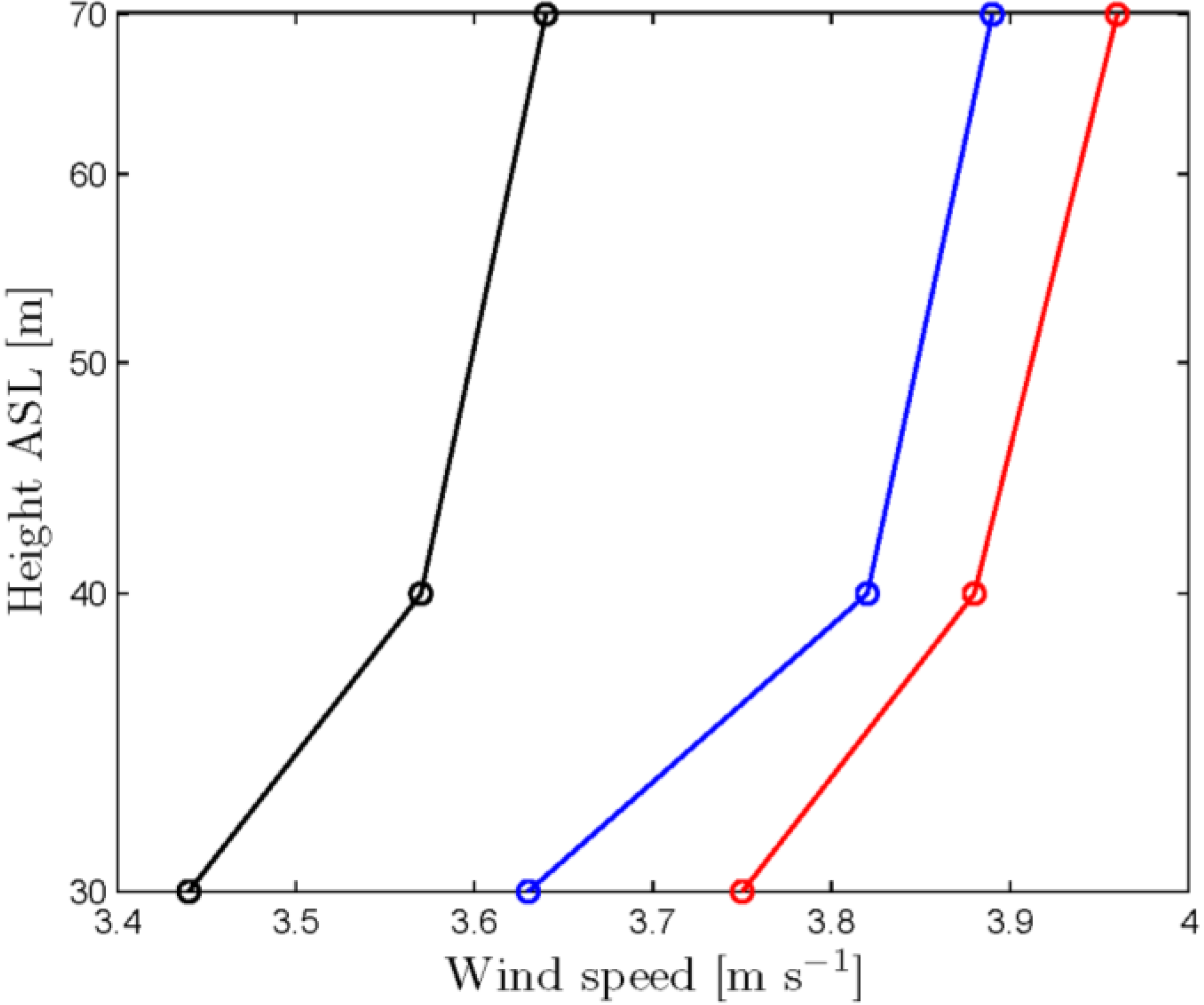
Figure 10). M7 is located 4 km east of M6. The wind profiles from M6 are graphed in
Figure 6 for three 10-min periods: Before, at and after the photographs. The wind profiles show slightly unstable conditions. Furthermore, the turbulence intensity is observed to be ~17% at 70 m, ~16% at 40 m and ~18% at 30 m which also indicates unstable conditions. The observations from 70 m are from a top-mounted cup anemometer whereas the observations from 40 m and 30 m are from boom-mounted cup anemometers at the northwest booms (see [
10] for details). Thus the wind speed and turbulence intensity data may be influenced by the mast and booms.
Figure 6.
Wind profiles observed at M6 on 12 February 2008 at 10:00 UTC (red), 10:10 UTC (black) and 10:20 UTC (blue) at three heights above sea level (ASL). Data are from DONG Energy and Vattenfall.
Figure 6.
Wind profiles observed at M6 on 12 February 2008 at 10:00 UTC (red), 10:10 UTC (black) and 10:20 UTC (blue) at three heights above sea level (ASL). Data are from DONG Energy and Vattenfall.
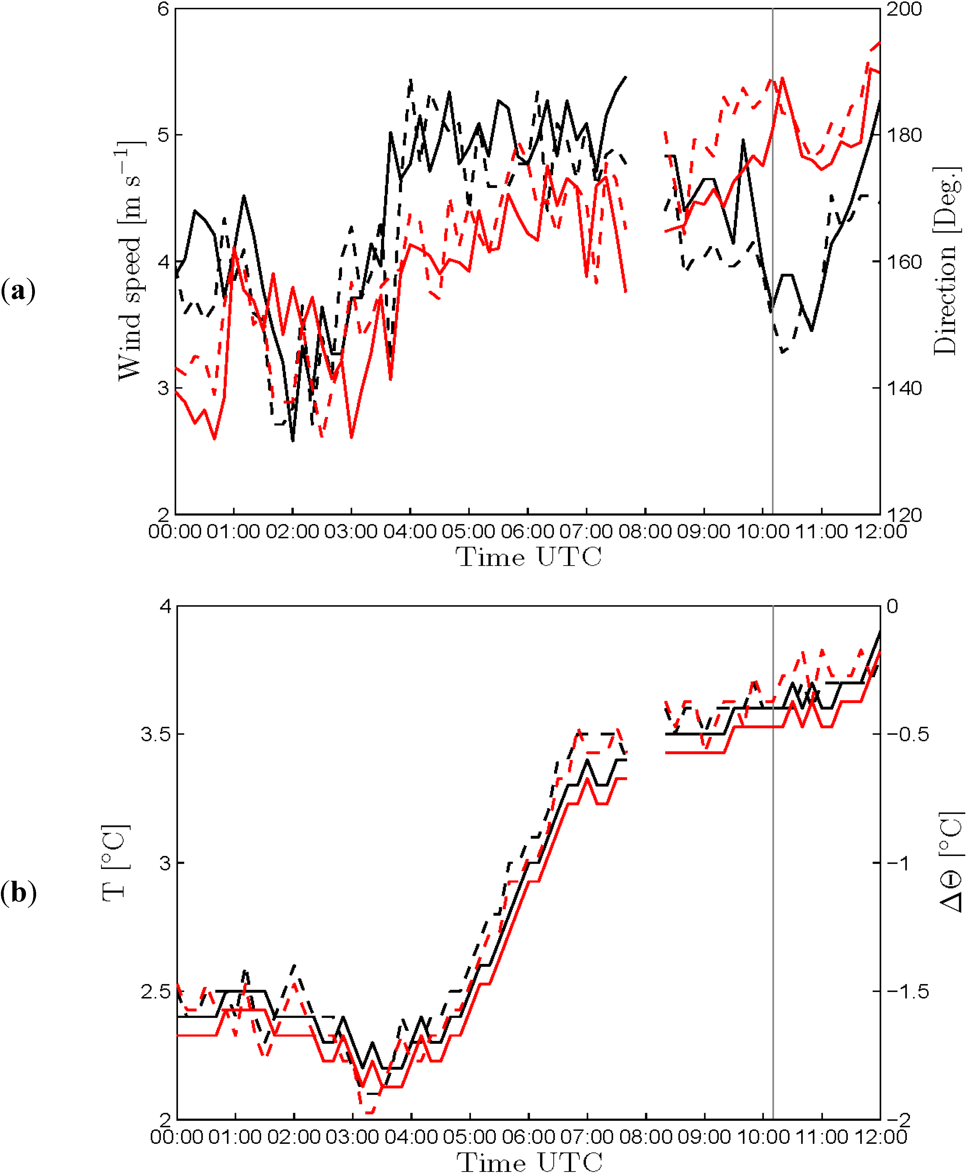
Figure 7 shows the wind speeds, wind directions, air temperatures, and the potential temperature difference from midnight to noon on 12 February 2008. The wind speeds are nearly constant and low, ~4–5 ms
−1, whereas the wind directions change from ~140° to ~190°. During the night the air temperatures are below 2.5 °C. From 5:00 to 7:00 UTC the temperatures increase one degree and thereafter the air temperatures are nearly constant ~3.5 °C. The water temperature at 3 m depth is constantly 4.7 °C (not shown) but the potential temperature difference between 64 m and −3 m is shown and the case is seen to be unstable. The pressure is ~1037 hPa and constant (not shown). For all parameters observed there are very little differences between observations from M6 and M7. At both masts air temperatures at 16 m are observed and the potential temperature difference between 64 m and 16 m is nearly constant ~0.2 °C before 6 a.m. and thereafter nearly constant ~0.1 °C (not shown). The local unstable conditions indicate that the stability decreases from a wet-adiabatic to a near dry-adiabatic layering. The fog that had covered the entire area is disappearing due to this change in the adiabatic situation. The thinning of the fog takes place from the top towards the bottom of the inversion. Only sea smoke in a shallow layer of 5 to 10 m near the ocean surface remained (
Figure 2). [
3] described the sea smoke as a result of a colder humid air advected over a warmer sea surface. This explanation is supported by the meteorological observations near the wind farm. During the entire morning the air temperature remained lower than the sea temperature, and vertical mixing to a certain height might easily be achieved. Selected data from M6 are listed in the
Appendix.
4. Wake Model Results from CFD DES
The distance in the turbine wakes at which the first condensation takes place is around 50 to 100 m downstream centered at the nacelle position (
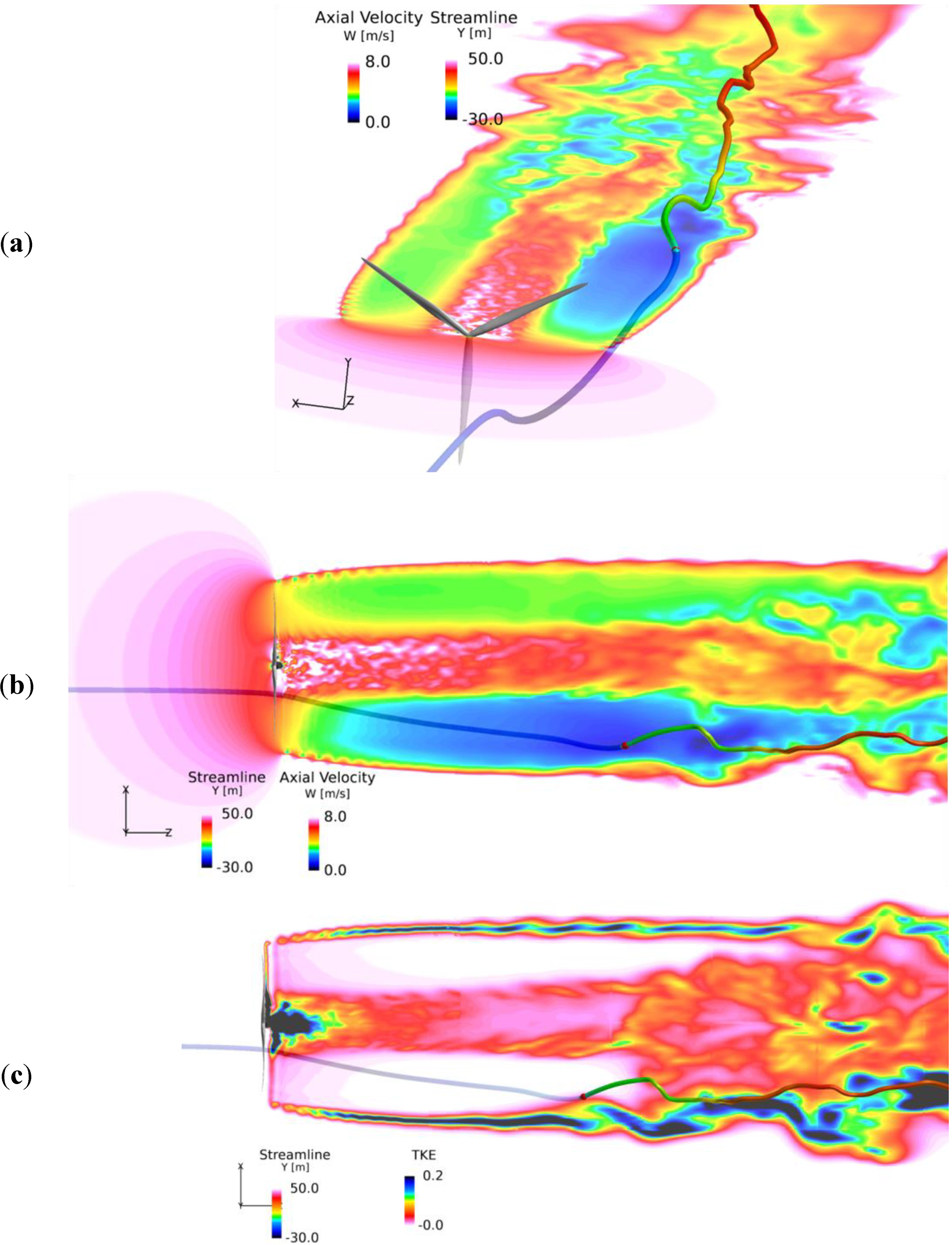
Figure 2). To gain further insight to the physical properties in the turbine wake field, CFD model results on axial velocity, turbulent kinetic energy (TKE), vertical velocity and pressure are investigated.
Figure 7.
Meteorological conditions observed at M6 and M7 during 12 h on 12 February 2008. (a) Upper panel: Wind speeds at M6 (––) at 70 m and M7 (- -) at 60 m. Wind directions: M6 () and M7 () both at 68 m; (b) Lower panel: Air temperatures at M6 (––) and M7 (- -) both at 64 m. Potential temperature difference between 64 m and −3 m at M6 () and M7 (). The thin vertical line indicates the time of the photographs. Data are from DONG Energy and Vattenfall.
The result on the axial velocity in the wake from the simulation with a full rotor DES (with an overset mesh method) of a NEG Micon NM80 turbine in clock-wise rotation with a velocity at hub height of 8 ms
−1 and with a vertical shear on the axial wind velocity is shown in
Figure 8. For more information about the simulation see the original article for which the simulation was carried out [
11]. The streamline visible shows how a mass of air located under the hub height of the rotor would be displaced to a higher position vertically due to the wake rotation.
Figure 8.
Wake development model results using Detached Eddy Simulation of a full rotor simulation in laminar inflow. The axial velocity and turbulent kinetic energy (TKE) are shown using a transparent color count in the plane. The streamline is centered at the maximum wake deficit and shows that the flow is following the wake rotation, bringing up air with lower velocities. (a) Upper panel: The axial velocity in the horizontal plane at hub height viewed in slant range from above; (b) Middle panel: The axial velocity in the horizontal plane at hub height viewed from nadir; (c) Lower panel: TKE in m2 s−2 viewed as in (b). The rotor is located to the left. The turbine rotates clockwise and the wake rotates counter-clockwise.
The axial velocity appears to be lower on one side of the wake compared to the other. This effect is due to the wake rotation. Wake rotation moves air parcels with a lower wind speed located in the lower part of the rotor swept area upwards and moves air parcels with a higher wind speed in the upper part of the rotor swept area downwards. The strongest rotation is in the central region of the wake [
Figure 8(a,b)].
TKE is also highest in the central region of the wake [
Figure 8(c)], but TKE decreases much more rapidly downwind than the axial velocity. Furthermore it may be noticed that TKE is high near the tip of blades and increases in strength and width downwind whereas the axial velocity shows a more constant development downwind at the tip of blades.
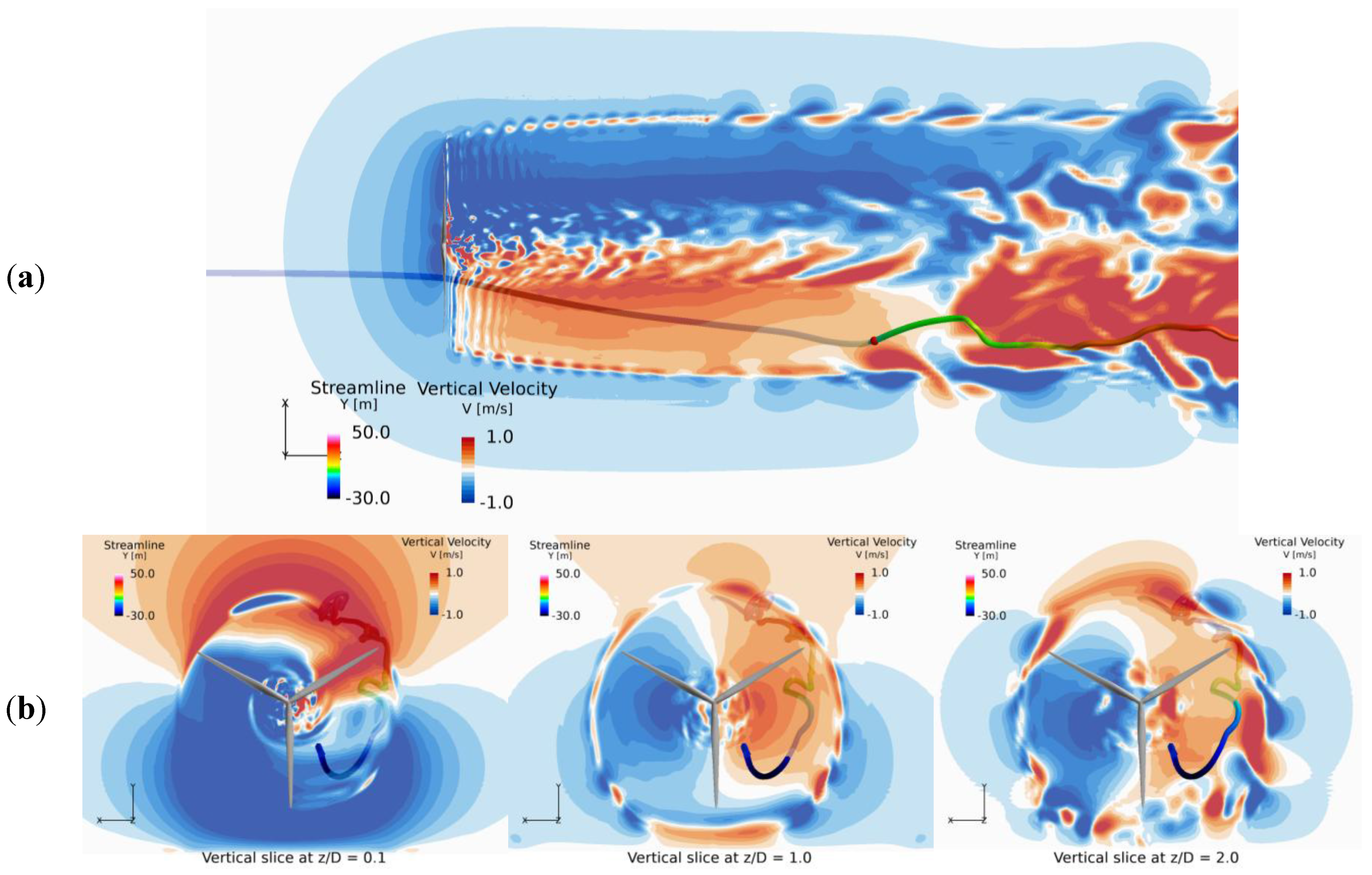
The graphics on vertical velocity (
Figure 9) show in which vertical direction the rotation is occurring. The three dimensional pattern is characterized by strong upward winds near the rotor at a distance of 0.1 rotor diameter (
i.e., 8 m downwind) above the horizontal hub height plane. Further downwind the upward velocity includes a much deeper layer of the rotor swept area even stretching out beyond the tip of blades. However, the turbulent structure also causes patches of downward winds to appear, in particular, in the outer regions of the wake.
Figure 9.
Wake model results from the full rotor DES model of the vertical velocity. The red color indicates air moving upwards while the blue color indicates air moving downwards. The streamline is centered at the maximum wake deficit. (a) Upper panel: The vertical velocity in the horizontal plane at hub height viewed from nadir. The rotor is located to the left; (b) Lower panel: The vertical velocities are shown in the vertical plane of the rotor swept area at three different downwind locations: Left at 0.1 rotor diameter distance, middle at 1 rotor diameter distance, and right at 2 rotor diameter distance. The turbine rotates clockwise and the wake rotates counter-clockwise.
At the distance of 1 rotor diameter (80 m) there is a near perfect symmetry with upward winds at the one side and downward winds at the other side with a gradual decrease in magnitude in winds from the centre of the hub towards the tip of blades. At the distance of two rotor diameters (160 m) the turbulence clearly erodes this symmetry and redistributes the air parcels to a more complex structure. The turbulent imprint to this large-scale wake structure is more pronounced further downwind.
The pressure drop in the wake from the DES simulation is found to have its maximum value very close to the rotor. The pressure increases downwind with the relatively lowest pressure remaining at hub height behind the nacelle but at a distance of 1 rotor diameter the pressure depression is modest. The pressure drop near the tip of blades is localized and the pressure quickly increases downwind (not shown).
In the wind turbine control regime below rated wind speed both the NM80 pitch controlled turbine and the Vestas V80 pitch controlled turbine at the Horns Rev 1 wind farm, would typically have a constant tip speed ratio (velocity of the tip of the blade divided by the incoming wind speed). Furthermore, for wind speeds lower than or equal to 8 ms−1 the thrust coefficient is nearly constant. It means that the wake deficit ratio will also be equivalent for velocities lower than 8 ms−1. These two parameters combined give us confidence that the state of the wake of the NM80 wind turbine simulated at 8 ms−1 is of similar nature as the wake of the V80 wind turbine at 4 ms−1.
5. Wind Farm Wake: Observations
The SCADA data from the Horns Rev 1 wind farm is used to identify the most likely time of the photographs during the morning of 12 February 2008. The sun angle appears to be slightly before noon as seen on the sunlight on the fog. It is noted in
Figure 2a that one wind turbine (“88”, see
Figure 10) in the southern row was not operating. The SCADA information reveals that this turbine “started/stopped” (a status where the wind turbine starts and stops one or more times within a period) in the interval between 10:00 UTC and 10:10 UTC and had this status during the following 50 min. In addition, checking the status of all other turbines in this 50 min time interval allowed the identification. For the first 10-min time interval only, all other turbines in the southern row were operating. SCADA information from turbine “48” is missing throughout.
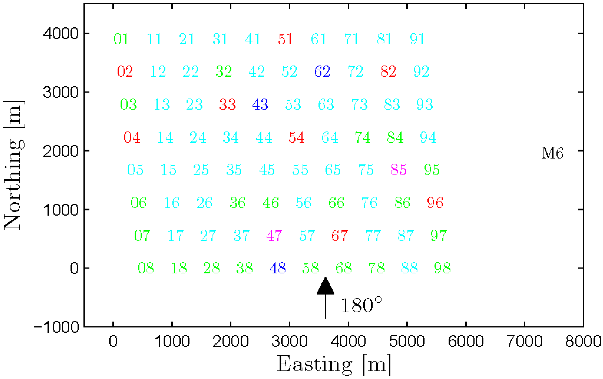
Figure 10 shows the status of all turbines at the relevant 10-min interval. The wind direction of 180.8° observed at M6 at 68 m confirms the wind direction near hub-height of all turbines in the southern row.
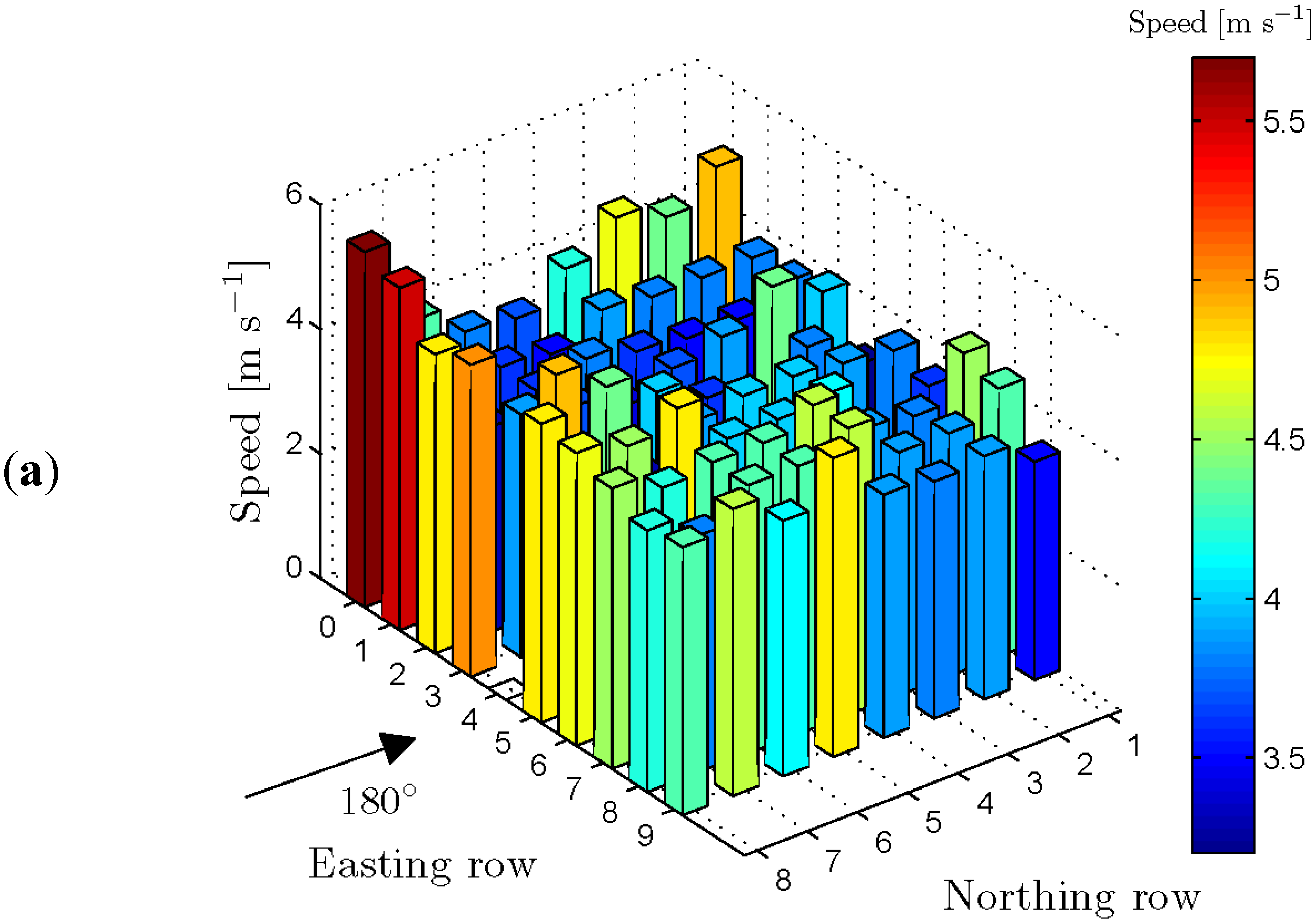
The wind speed observed at M6 at 70 m is 3.64 ms
−1. This is lower than the nacelle wind speed at all turbines in the southern row that all experience free stream velocity [see
Figure 11(a)]. The nacelle wind speeds in this row show a clear decrease from west to east and the low winds observed at M6 supports this general trend. In
Figure 11(a) it is clear that winds at turbines located north of “rotor stopped” turbines are relatively higher.
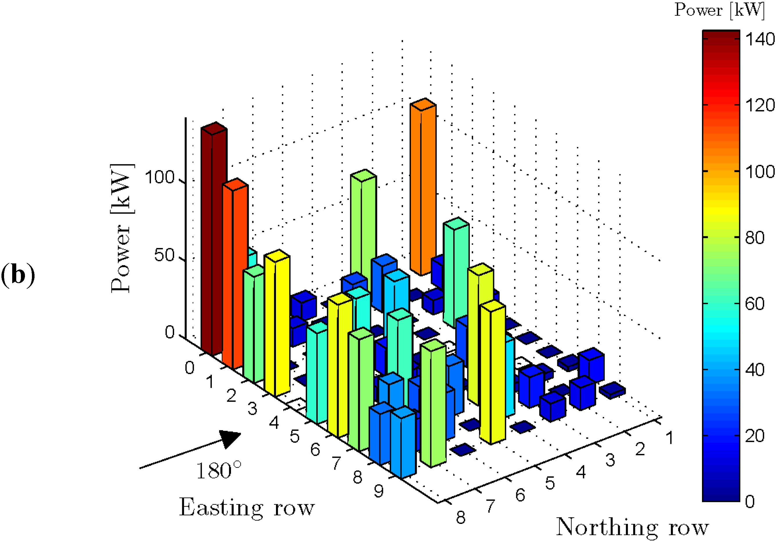
The turbines with relatively high production are those in the first row and turbines located downwind of stopped turbines [
Figure 11(b)]. Compared to the rated power of 2 MW, the amount of power of the turbines producing the highest, up to 140 kW, is very low. All turbines in the southern row operated at 13.5 revolutions per minute (RPM) except turbine “88” that was slowing down. No SCADA data on turbine “48” is available but seen from the photographs this wind turbine did operate. In contrast, most other turbines in the wind farm operated slower. Selected SCADA data are listed in the
Appendix.
Figure 10.
The Horns Rev 1 wind turbine layout with numbering and color identification for operating status at 10:10 UTC on 12 February 2008: Green: operating; Pale blue: start/stop; Red: rotor stopped; Magenta: faulty scan or power down-regulated; Dark blue: no SCADA information. The position of the meteorological mast M6 is also indicated. The first digit in the number indicates the west-east row and the second number indicates the north-south row. Data are from DONG Energy and Vattenfall.
Figure 11.
The Horns Rev 1 data from 12 February 2008 at 10:10 UTC from SCADA data. (a) Upper panel: Nacelle wind speeds; (b) Lower panel: Measured power. Data are from DONG Energy and Vattenfall.
Figure 11.
The Horns Rev 1 data from 12 February 2008 at 10:10 UTC from SCADA data. (a) Upper panel: Nacelle wind speeds; (b) Lower panel: Measured power. Data are from DONG Energy and Vattenfall.
6. Discussion
The fog formation at the Horns Rev 1 wind farm photographed from a helicopter in the late morning on 12 February 2008 is due to special atmospheric conditions. Light winds prevailed from the southeast for many hours; thus the radio-sounding observations from Schleswig 150 km southeast of the Horns Rev wind farm are used to assess the vertical air mass in regard to temperature, humidity, wind speed and direction at the upper levels.
Local observations from the wind farm are used to characterize the conditions at the lower levels at the specific time of the occurrence of the fog. The wind and temperature profiles reveal unstable conditions. The local turbulence intensity also indicates unstable conditions. The combined data allows us to conclude that a humid cold air mass is located above a warmer ocean surface and that adiabatic cooling takes place aloft. Earlier in the same day fog or low-laying clouds most likely covered the area but at the time of the photographs only the sea smoke persisted. The explanation for the fog formation in the wake of the wind turbines given by [
3] is that two vertical layers of saturated air masses with different temperatures are mixed. In our view the process for the fog formation is adiabatic cooling in the upper part of the swept rotor area. If so the assumption of two contributing air masses seems unnecessary.
The triggering condition for re-condensation into fog in the wake is due to the wind turbine operation. The turbines operate near the cut-in wind speed (4 ms−1). The rotors in the southern row of turbines operate at 13.5 RPM except turbine “88”. The operating rotors cause upward air movements of humid warm air from near the sea surface and downward movements of dry-adiabatically cooled air at the top of the rotor some distance downwind from the turbines. The fog appears to be mainly present in the downwind wake areas where the axial wind speed and turbulent kinetic energy are high as indicated by the CFD DES model results.
It can be noticed in the photos that the initial point for fog formation is approximately at hub-height and around 50 to 100 m downwind for each of the fully operating turbines. So apparently the axial rotation of winds needs to take place through a certain period of time (~22 s) before water droplets (fog) starts to form from the super-saturated water vapor enhanced by the rotating winds. The initial condensation seems to occur in the counter-rotating swirl generated by the rotor. In other words, the induced velocities perpendicular to the wind direction are largest at the root section of the blade and this means the flow is rotating most here. The counter-clockwise swirl is lifting up warm humid air from the lower parts of the rotor to a higher level, where it is cooled down and condensation is accelerated. There is also a pressure drop in this region but of rather low intensity so the turbulent mixing is probably the most important factor.
The area with fog expands downstream as the individual wakes spread in the vertical and transversal directions and the neighboring bands of fog blend at a distance of around 2 km downwind. According to [
12] the power deficit at Horns Rev 1 is found to be maximum at the range of wind speeds 3–5 ms
−1 and the wake expansion is large (29°).
In [
3] the fog structure is explained from the unstable temperature stratification of the air leading to the slightly bumpy nature of the wake clouds. In contrast, we find that the large-scale structure of the fog has a clear imprint from the wake flow dynamics with rotational spiraling bands. This is based on the axial velocities and turbulent kinetic energy development downwind from the CFD DES wake model results.
The SCADA data from Horns Rev 1 is used to identify the most likely time of the photographs. Furthermore, the SCADA data shows the production is low as the wind speed is near cut-in. The meteorological observation of wind speed at M6 is even lower. It has previously been documented that coastal wind speed gradients are found near Horns Rev using satellite synthetic aperture radar (SAR) wind maps and modeling [
13]. Also in [
14] and [
15] satellite and airborne SAR wind observations showed wind speed gradients locally in and near the Horns Rev 1 wind farm.
The Horns Rev 1 wind farm wake has previously been modeled successfully with wake engineering models in the wind speed ranges 8 ± 0.5 ms
−1 [
16] and down to 6 ms
−1 [
17]. The thrust coefficient is high in low winds [
12] and the resulting wake-disturbed wind speeds are sufficiently low to stop the downstream turbines. As the wake meanders downwind the start/stop phase of the turbines might happen several times during the 10-min period. This dynamical effect is pretty difficult to model.
The wake engineering models assume a constant wind speed over 10 min. Thus an engineering wake model cannot capture neither the wind speed gradient, nor the dynamical changes of meandering wakes. Furthermore, for a wind speed of 4 ms
−1 it will take around 15 min for the flow to pass the entire wind farm. The PARK model [
18] was run for the present case (the results are not shown) and the agreement with the produced power was not so good. The engineering wake models are calibrated for higher wind speeds where most wind farm power production takes place. This very special wake case may possibly be modeled in the future including stability effect. SCADA data for comparison to future model results are listed in the
appendix.
The photographs of the fog formation in the wake of the Horns Rev 1 wind farm are often shown at wind energy events. It is recommended to be cautious on the interpretation of this wake as it is in fact not a typical wind farm wake situation at all. Only few turbines within the wind farm operated normally. The wind speed was so low that only the wind turbines in the front (southern) row except turbine “88” rotated at 13.5 RPM. Turbine ‘88’ and most other turbines in the wind farm operated at less RPM. The fog is most likely caused mainly by the accelerated condensation in the counter-rotating wake swirl generated by the turbines in the front row.
7. Conclusions
The case of fog formation at the Horns Rev 1 wind farm that occurred 12 February 2008 at 10:10 UTC and was photographed from a helicopter is examined. The special atmospheric conditions are characterized by a layer of cold humid supersaturated air that re-condensates to fog in the wake of the turbines. The process is fed by humid warm air up-drafted from below and adiabatic cooled air down-drafted from above by the counter-rotating swirl generated by the rotors. The wind speed is near cut-in and most turbines produce very little power. The condensation appears to take place primarily in the wake regions with relatively high axial wind speed and high turbulent kinetic energy. The large-scale structure of the fog has an imprint of rotational spiraling bands similar to wake flow characteristics deduced from CFD DES modeling.

 ,
, 


