Development of a Transient Model of a Stirling-Based CHP System

Abstract

Although the Stirling engine was invented in 1816, this heat engine still continues to be investigated due to the variety of energy sources that can be used to power it (e.g., solar energy, fossil fuels, biomass, and geothermal energy). To study the performance of these machines, it is necessary to develop and simulate models under different operating conditions. In this paper, we present a one-dimensional dynamic model based on components from Trnsys: principally, a lumped mass and a heat exchanger. The resulting model is calibrated using GenOpt. Furthermore, the obtained model can be used to simulate the machine both under steady-state operation and during a transient response. The results provided by the simulations are compared with data measured in a Stirling engine that has been subjected to different operating conditions. This comparison shows good agreement, indicating that the model is an appropriate method for transient thermal simulations. This new proposed model requires few configuration parameters and is therefore easily adaptable to a wide range of commercial models of Stirling engines. A detailed analysis of the system results reveals that the power is directly related to the difference of temperatures between the hot and cold sources during the transient and steady-state processes.

1. Introduction

A cogeneration system simultaneously provides heat and power. Although these systems are extremely interesting for isolated circumstances, these configurations have become increasingly important during recent years because of the increases in their energetic efficiency and reliability. Thus, these systems will reduce carbon dioxide emissions into the atmosphere due to the improvement in fossil fuel utilization, reduction in energy transport losses, and waste heat recovery [1]. This system is expected to increase the performance and reduce the pollution of internal combustion engines (ICE) and micro-turbines [2].

Stirling engines (SEs) are reciprocating external combustion devices that can operate using almost any type of heat source. There have been significant efforts to develop SEs activated by solar energy [1,3] or any other type of renewable energy, such as biomass [4] and biodiesel. SE work independently of the heat source because the internal gas runs within a thermodynamic cycle as long as the temperature difference between the hot and cold sources is maintained.

SEs normally use hydrogen, nitrogen, helium, or air as the working fluid for the heat exchange within the regenerative thermodynamic cycle [1]. The selection of the fluid will principally depend on the operating temperature ratio of the hot and cold sources, the required power output, and the working pressure [1].

Other advantages of the SE are its noiselessness compared with ICE or micro-turbines and the possibility of its use in residential buildings because this combined heat and power (CHP) system presents an output power that is appropriate for typical family homes during winter periods. This overview confirms that SEs will continue to be developed and investigated to attain new renewable and distributed generation capacities.

Some ICE devices also present trigeneration capacities [5,6], incorporating a heat pump system that can generate cooling during summer periods. Depending on the weather and building conditions, different CHP systems will be required.

As more investigations have focused on micro-cogeneration devices, different validation models have been proposed in the literature [4,7,8]. Most of the models were developed under steady-state conditions, as in our previous work [9], but transient responses are needed and useful for real HVAC simulations because the heating and domestic hot water systems are frequently turned on and off throughout the year.

The annual efficiency of an SE installation can be estimated using steady-state models. However, a heating system generally operates under dynamic conditions with controllers that switch the system on and off, provoking different starts and stops depending on the external operating conditions. Therefore, dynamic models are more appropriate for certain types of simulations, although they present disadvantages that depend on the type of SE being modeled and must be developed for each type of SE.

Existing models usually simulate specific models of the SE, as in [4,8], or use the Annex 42 model [10]. This method was developed by the International Energy Agency (IEA) and is used to simulate cogeneration devices integrated in building simulation tools [7] starting from empirical data and parametric analysis to obtain the output data, which is implemented in different simulation tools. Another method involves the development of an easily customizable model using information obtained from different experiments [11].

More exhaustive analyses study the dynamic behavior of the machine and search for an optimum design base from a thermodynamic point of view [12,13], taking into account the different mechanical and thermodynamic losses associated with the dead volume and the non-ideal regeneration principle [14,15].

The necessity of the model proposed below arises from the fact that defining a more complex model usually requires a thorough analysis of design parameters that are often unknown, such as the heat exchange surfaces, heat transfer coefficients, and manufacturing material properties, causing the use of these models to be limited. Furthermore, simple models are easier to port between different engines, which reduces the calibration requirements [16].

Thus, the new functional model was easily calibrated without time-consuming invasive techniques, as described in the following sections. The software GenOpt 3.1.0 was used to perform the optimization because it minimizes the cost function calculated using a different simulation program [17].

Using lumped-mass transient models, different SE operating parameters have been evaluated, and their influence on the behavior of the engine was investigated [16,18]. These lumped parameter models are a valid method [19] to successfully simulate the transient performance of different thermal machines.

Therefore, this paper presents an optimized lumped model that simulates the transient performance of SE devices while taking into account the start-up and shutdown periods within the software simulation environment.

2. Experimental Apparatus

The validation of the proposed lumped model was conducted in a commercial SE device. The manufacturer is Whisper Tech Limited (Wellington, New Zealand), and the unit is a Whispergen DC personal power station, model PPS16-24MD, a double-acting alpha-type four-cylinder SE. This engine runs on diesel and was originally built as a battery charger, although similar engines are sold as substitutes for condensing boilers in residential homes. Although both heating systems present similar efficiencies, the SE configuration produces extra electrical energy.

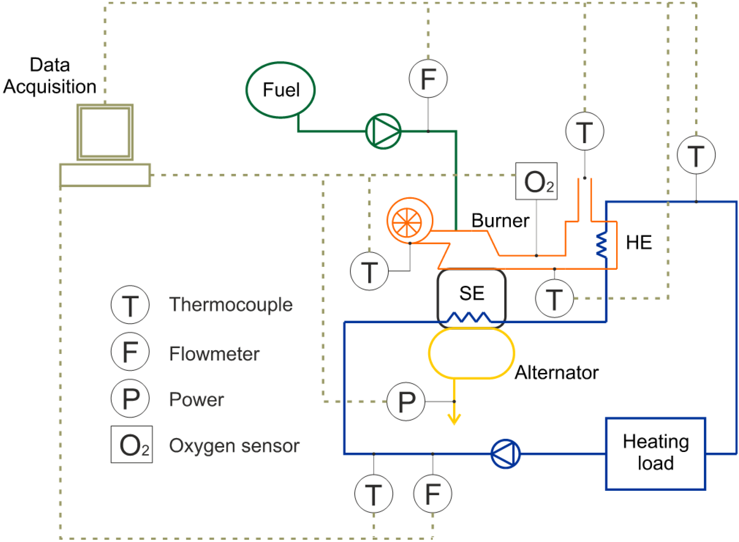
The engine has a block with four interconnected cylinders filled with nitrogen at a maximum pressure of 28 bars at 70 °C. The continuous compression and expansion of the nitrogen displaces the cylinders up and down, and this movement is converted into rotational movement via a wobble-yoke mechanism. To test the engine, an experimental plant was constructed. This cogeneration system incorporates different interconnected components, primarily including a burner, an alternator, a four-cylinder SE, and an exhaust heat exchanger. Furthermore, the SE experimental apparatus contains different sensors spread over the plant, as shown in Figure 1.

Figure 1. Data acquisition from different sensors in the experimental plant.

Figure 1. Data acquisition from different sensors in the experimental plant.

The software program Micromon V1.0 was used to collect the data produced by the SE. An interface programmed in LabVIEW recorded the information from the PT100 temperature sensors distributed throughout the installation. The water flow rate and the temperature of the water flowing into the SE and out of the heat exchanger (HE) were measured using a Sensonic II heat meter. This system combines a volumetric flow meter through an electronic impeller wheel scanner and temperature sensors. The data from the sensors were collected each minute during the entire test.

This SE is a thermal machine in which the combustion chamber acts as the heat source and the water from the heating system corresponds to the cold source. A water pump and air blower maintain circulation of the water and gases, respectively. The heating load is simulated by a radiator and a fan coil with a variable speed control blower that maintains the temperature of the cold source below a preset value. This value can be modified between 45 and 70 °C to enable the cogeneration system to be adapted to different heating configurations.

3. Working Principle

The performance of the SE is principally controlled via the air flow and the quantity of fuel entering the combustion chamber.

A temperature sensor and an oxygen sensor are placed between the engine’s burner and exhaust HE, as is represented in Figure 1. This oxygen sensor measures the O₂ content in the exhaust gases. This information is used to continuously adjust the fuel pump to maintain the fuel-air ratio around a prefixed set point, as is explained in Farra et al. [20].

Furthermore, the temperature sensor indicates whether the set point temperature of 480 °C is reached. The air blower speed is constantly adjusted to reach the prefixed set point temperature, which was calibrated at the factory. When steady-state operation is achieved during the experiments, the air blower runs at maximum speed (rpm) trying to reach the set point temperature. Due to the air blower capacity, the burner temperature during steady state increases to 460 °C, and the prefixed set point is not reached.

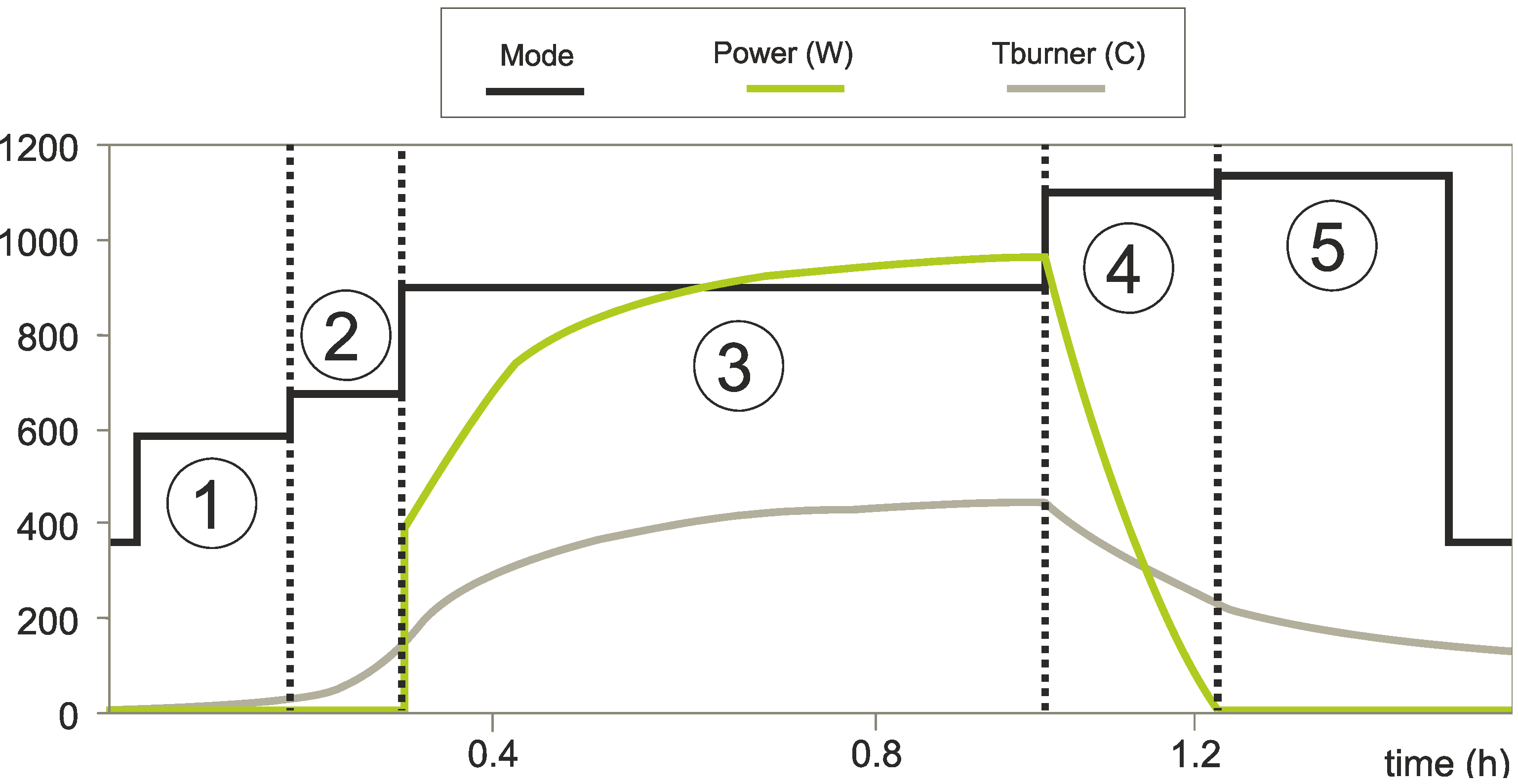
The SE starting, running, and stopping modes follow a methodological process in which the switching points are determined by time or temperature set points. The most representative modes are illustrated in Figure 2. During mode 1, the SE examines the different instrumentation from the cogeneration system and turns on a glow plug to preheat the combustion chamber. In mode 2, the fuel starts to feed the combustion chamber. When the temperature from the burner reaches 145 °C, the mode changes to mode 3, and the SE starts to turn. During this mode, the SE operates in the running mode, and power and heat are obtained from the fuel. Mode 4 starts when the stop button is pressed and the fuel supply is cut off. The alternator still produces power during this mode, but the rpms are drastically reduced. When the engine stops turning, it starts mode 5, and the SE dissipates the remaining heat within the block.

Figure 2. Operating modes.

Figure 2. Operating modes.

4. Modeling

4.1. Lumped Model

A lumped capacitance model with two lumps is used to represent the thermal behavior of the different parts of the SE. To calculate the changing temperature over time, Equation (1) is solved:

$$\mathsf{\rho }·\text{V}·\text{c}·\frac{dT}{dt}=\dot{\text{E}}-\text{h}·\text{A}·({\text{T}}_{\text{lump}}-{\text{T}}_{\text{amb}})$$

(1)

where ρ is the density; V is the volume; A is the area; and c is the specific heat of the body. The energy input $\dot{\text{E}}$ is used to take into account the energy absorbed or transferred by the combustion chamber or the engine’s block. The convection term on the right side of Equation (1) represents heat losses to the environment.

4.2. SE Model Description

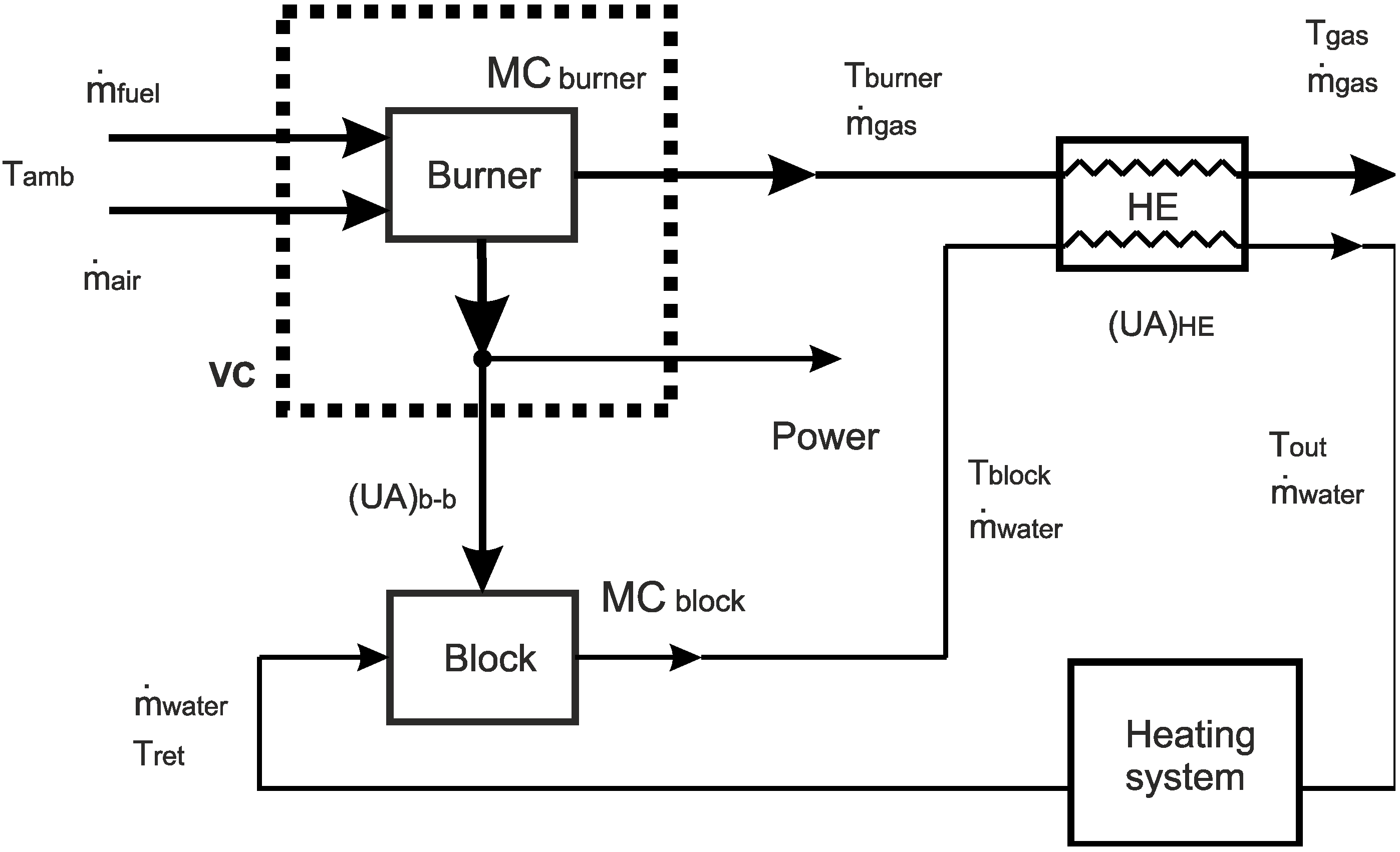
The principal participant energy and mass flows inside the SE cogeneration system are depicted in Figure 3. According to this figure, the global system can be subdivided into three principal parts differentiating a lumped burner model, a lumped block model, and an exhaust heat exchanger.

As shown in Figure 3, air and fuel flow into the combustion chamber of the SE, which is then heated by the combustion of the fuel. This fuel is diesel with an LHV of 11.89 kWh/kg. In the burner outlet, a mass flow of combustion gases ṁ_gas at temperature T_burner is obtained. These gases heat the cylinder heads and consequently the nitrogen inside the block. The group formed by the burner and nitrogen is simulated via a lumped mass, which is represented in Figure 3 with a dashed line. The bottoms of the cylinders are cooled by the water that circulates around the heating circuit. This part represents the engine block and is simulated by an additional lumped mass. When the difference in temperature between the cylinder heads and the bottom is high enough, the SE starts to turn. An additional exhaust heat exchanger between the burner output and the block output is used to recover heat from the exhaust gases.

Figure 3. SE diagram.

Figure 3. SE diagram.

Attending to the thermal domain, the various heat flows inside the SE can be related, with the diesel combustion responsible for the generated heat and the ambient air corresponding to the heat sink:

$${\dot{m}}_{gas}={\dot{m}}_{air}+{\dot{m}}_{fuel}$$

(2)

$$M{C}_{burner}\frac{d{T}_{burner}}{dt}={\dot{m}}_{fuel}LHV-{\dot{m}}_g{c}_{p_{gas}}\left(T_{og}-T_{ig}\right)-{\left(UA\right)}_{b-b}\left(T_{burner}-T_{block}\right)-Power$$

(3)

$$M{C}_{block}\frac{d{T}_{block}}{dt}={\left(UA\right)}_{b-b}\left(T_{burner}-T_{block}\right)-{\dot{m}}_{water}{c}_{p_{water}}\left(T_{block}-T_{ret}\right)$$

(4)

4.3. Trnsys Simulation

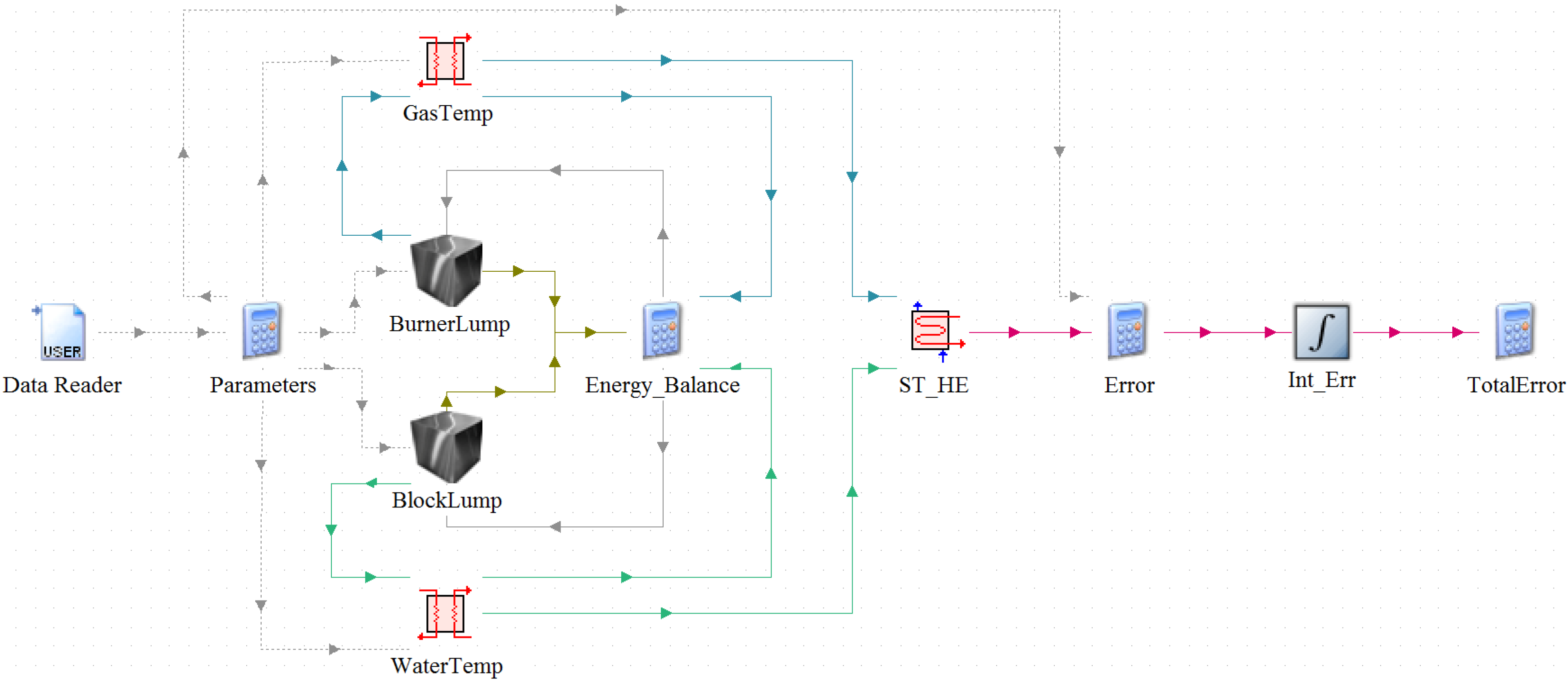
Consequently, a simple model based on components from the standard library of Trnsys was developed. First, a lumped mass was used to model the temperature changes produced by the entire engine during starting and stopping. A more exhaustive analysis showed that a lumped model with two lumps better simulates the behavior of the cogeneration device. These two lumped masses model a virtual temperature variation corresponding to the burner and block. The hot combustion gases heat the lump that models the burner, and the return water cools the lump that models the block through two separate heat exchangers. In addition, because the engine recovers heat from the exhaust gases, a shell and tube heat exchanger is used in the output, as shown in Figure 4. Finally, to complete the adjustment of the behavior model, three equations are used, in which the parameters are interpreted, energy balances are calculated, and errors are evaluated. Due to the simplicity of these components, implementing this model in other simulation tools, such as EnergyPlus or ESP-r, will be easy.

The lumped mass is modeled with Trnsys type 963, following Equation (1). The first lump models the burner temperature, which increases when the fuel is combusted. The second lump models the water block, which absorbs the burner energy and transfers it to the heating water. Finally, the shell and tube heat exchanger used to recover the heat from the exhaust gases is modeled with the corresponding Trnsys type 5, a zero-capacitance sensible heat exchanger.

Figure 4. Layout of the Trnsys simulation combining the three submodels.

Figure 4. Layout of the Trnsys simulation combining the three submodels.

Figure 4 presents a visual illustration of the Trnsys simulation developed in Simulation Studio. A data reader is used to supply the mass flow rates, the air and water temperatures, and the fuel supply. Two Trnsys equations are used to compute Equations (2) to (4).

By combining the different equations with the flows represented in Figure 3, Equations (5) and (6) are obtained:

$$Q_{comb}={\dot{m}}_{gas}·c_{p\_gas}·(T_{burner}-T_{amb})$$

(5)

$$Q_{water} = {\dot{m}}_{water}·c_{p\_ water}·(T_{block}-T_{ret})$$

(6)

4.4. Power Output Simulation

The model is completed by calculating the power produced in the alternator. Analyzing the thermodynamic cycle of an SE [21], the total work produced by an imperfect-regeneration SE with dead volumes during a cycle is defined in Equation (7):

$$W_{net}=mR\left[T_3\text{ln}\left(\frac{V_1+K{T}_3}{V_2+K{T}_3}\right)-T_1\text{ln}\left(\frac{V_1+K{T}_1}{V_2+K{T}_1}\right)\right]$$

(7)

where m is the mass of nitrogen; R is the constant of ideal gases; and K is a function of the dead volumes. As the dead volumes in our SE model are one- and two-orders of magnitude lower than the expansion and compression volumes, respectively, KT is negligible compared with V1 or V2, and the previous expression (7) can be reduced to Equation (8):

$$W_{net}=mR\text{ln}\left(\frac{V_1}{V_2}\right)(T_3-T_1)$$

(8)

Using engine speed n (Hz), the electric power can be calculated with expression (9):

$$Power=W_{net}·n$$

(9)

The engine heat exchangers from our SE were designed to work efficiently at a fixed value of revolutions per minute. This engine speed is controlled by varying the excitation electricity in the regulator, obtaining practically constant revolutions during the starting and stationary modes.

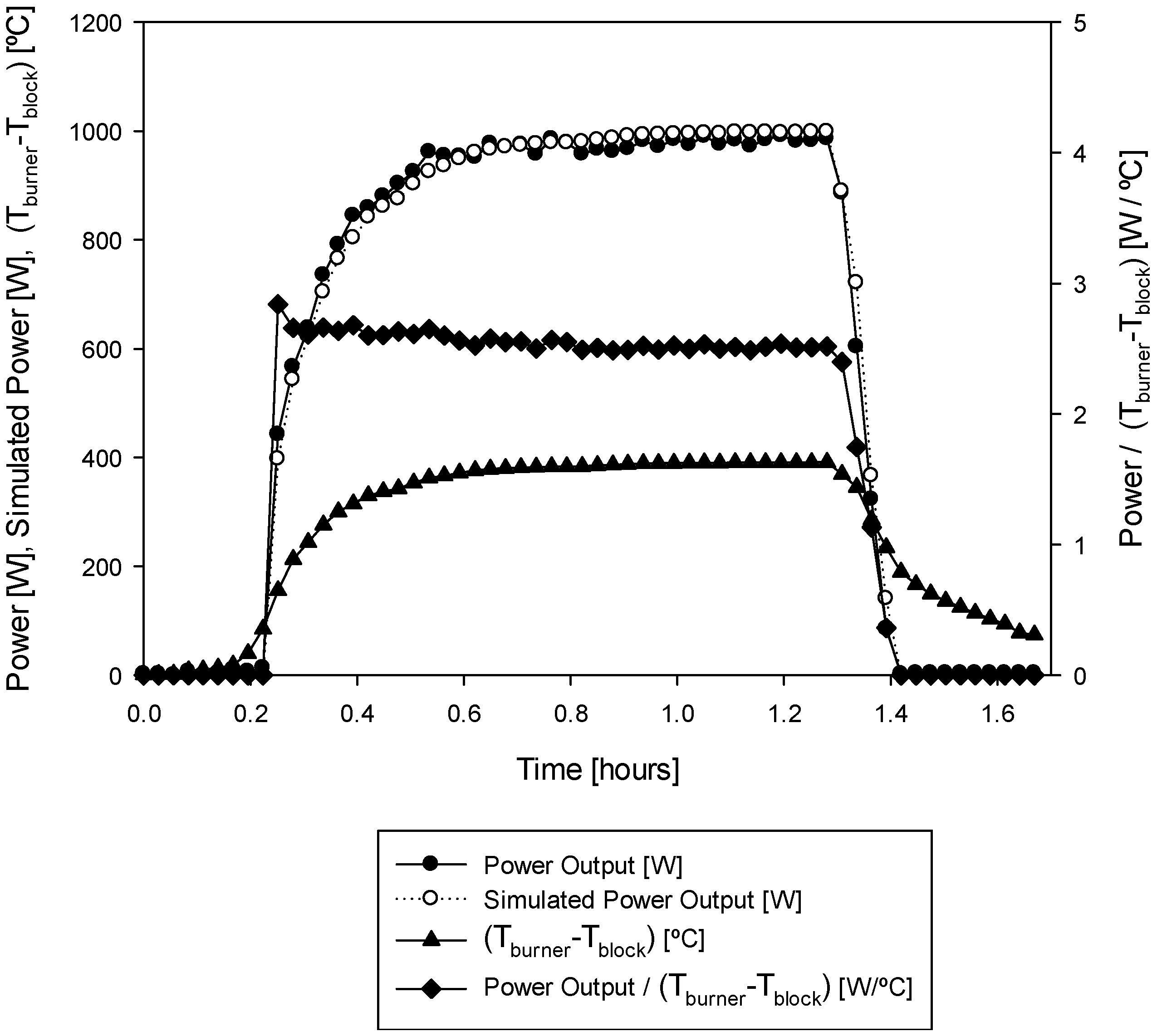
As demonstrated by the theoretical equations, the obtained electrical energy is experimentally shown to be directly proportional to the difference in the temperatures between the hot and cold sources. According to the experimental data, this relationship is 2.55, as represented in Figure 5. This relationship was maintained during the starting and stationary modes in the different experiments independently of the block temperature.

Figure 5. Simulated and experimental power output.

Figure 5. Simulated and experimental power output.

Furthermore, the shutdown process was simulated by interpolation between the power value when the shutdown button is pressed and zero when the temperature difference between the hot and cold sources is less than 190 °C; below this value, the engine stops turning. This approximation is used because the shutdown process is short and linear. Equation (10) was introduced in Trnsys to simulate the power production:

$$\begin{gathered} Power=gt\left({\dot{m}}_{fuel},0\right)*gt\left(T_{burner},150\right)*(T_{burner}-T_{block})*2.55+ \\ + eq\left({\dot{m}}_{fuel},0\right)*gt\left((T_{burner}-T_{block}),190\right)*\left(2.55*\frac{\left((T_{burner}-T_{block})-190\right)}{190}\right)*(T_{burner}-T_{block}) \end{gathered}$$

(10)

5. Experimental Data

A series of tests within the SE experimental apparatus was performed with the objective of comparing the results with the data obtained from the Trnsys simulation environment. Three tests with different set point temperatures for the cold source were performed. Because the CHP system allows the water temperature to be set between 45 and 70 °C, temperatures of 45, 60, and 70 °C were selected. The hot source temperature corresponds to the temperature of the burner and is preset to 480 °C. During the tests, the temperature of the hot source never reaches this value because as explained above, the control system regulates the fuel inlet according to the percentage of oxygen at the burner outlet. When the machine reaches steady state, the air supply fan is at 100% of its capacity, and the oxygen sensor and the pulse frequency of the fuel supply reach steady values, stabilizing the hot source temperature at approximately 460 °C.

Temperature, flow, and power data are measured with a sample rate of one minute, and the different tests have a total length of 90 min to ensure that steady state is reached.

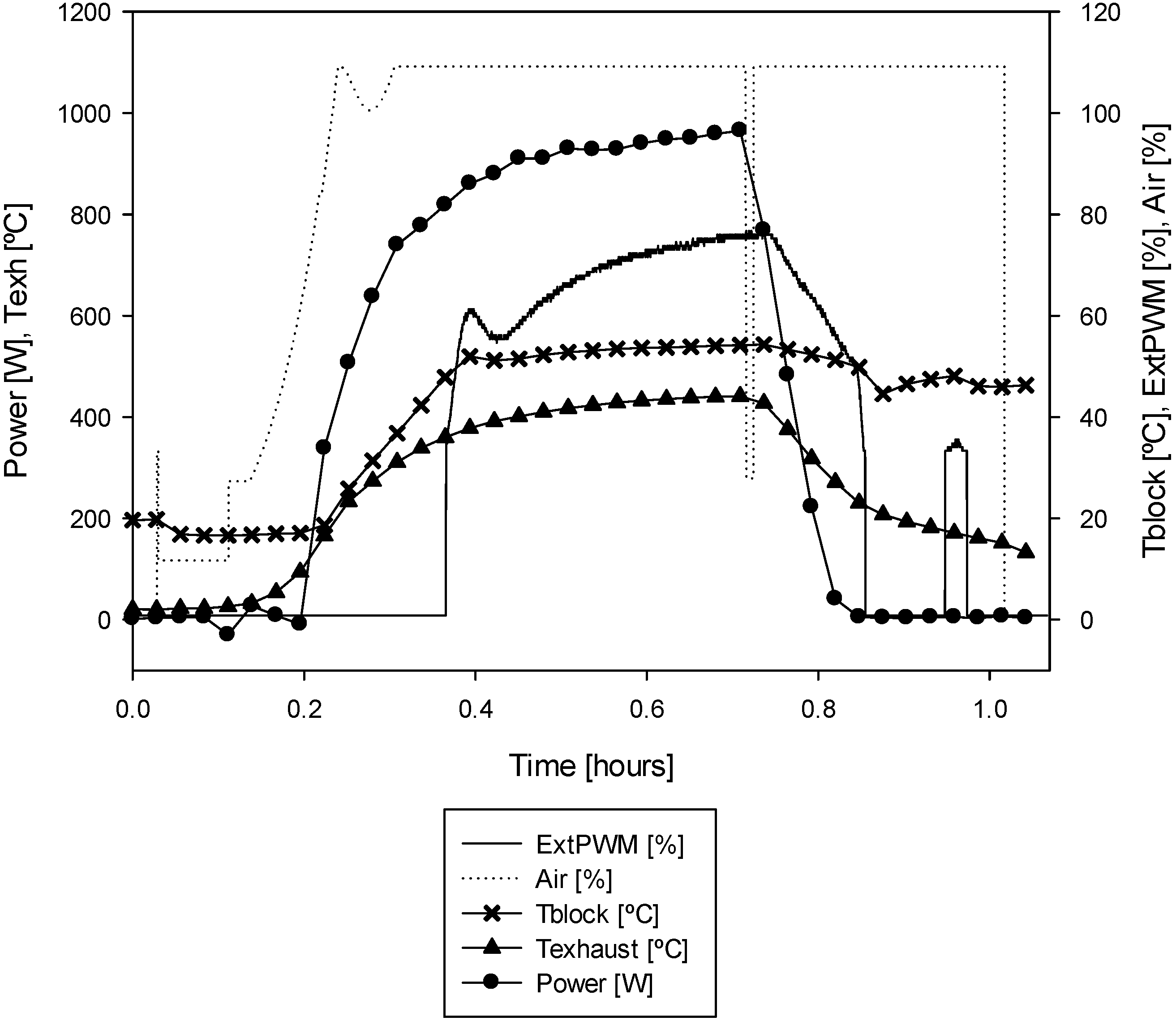
Figure 6 shows the various parameters collected with the Micromon software, which can be used to appreciate how the system regulates the water inlet temperature to the SE via the variable speed power control ExtPWM (external pulse width modulation) to maintain the preset block temperature set point. Thus, the difference in temperature between the cold and hot sources is maintained, and the smooth operation of the engine and the required temperature to supply the heating or DHW systems are ensured.

Figure 6. Obtained data from the SE.

Figure 6. Obtained data from the SE.

Moreover, at the time of SE shutdown, the air flow is interrupted for 30 s. This brief stop is translated as a temperature drop in the flue gas temperature sensor at the outlet of the burner.

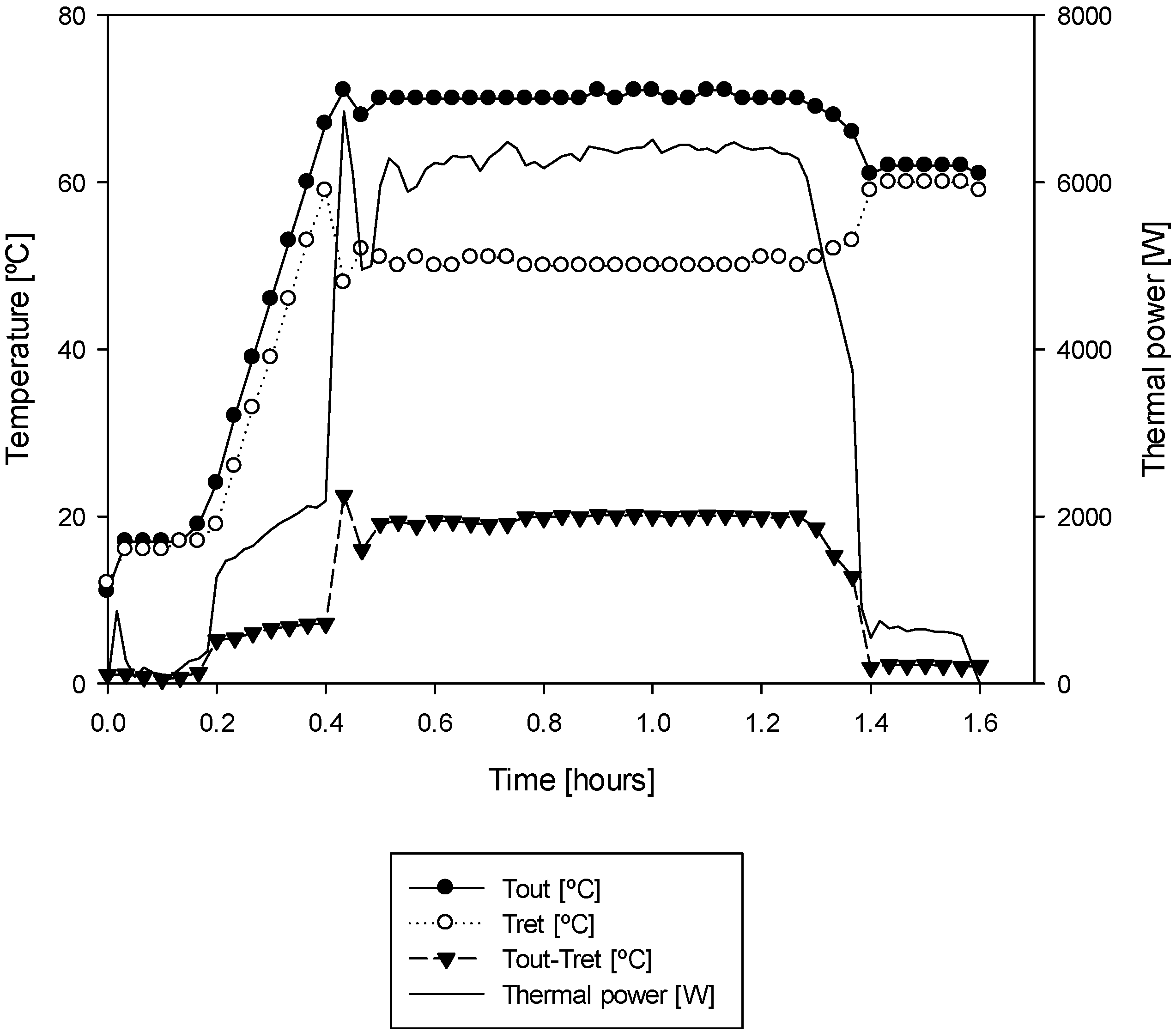
Figure 7 shows the input and output temperatures of the water in the SE. For approximately 10 min, the fuel is not injected into the combustion chamber, and the temperature of the heating water does not increase. From the moment at which combustion is initiated, the ramp in the increasing temperature lasts for 16 min, after which point steady state is reached and a thermal power of 6.14 kW on average is generated.

Figure 7. Thermal power and input and output water temperatures.

Figure 7. Thermal power and input and output water temperatures.

6. Model Calibration

The software GenOpt is a generic optimization program that minimizes the user-supplied cost function using a specific algorithm. Moreover, it is a single objective optimization program that can be run with almost any simulation software.

To optimize the cost function, GenOpt varies a certain number of variables. These variables within the study can be either continuous or discrete. To obtain the best result, an appropriate optimization algorithm and an adequate optimization function should be selected.

When the optimization process is started, GenOpt initializes the variables under study, and as the results of the function to be optimized are obtained, the program adjusts the values of different parameters within the established limits to achieve an optimal value for the function under study. GenOpt uses different text files that define the parameters that can vary, their preset limits, the location of the function to be optimized, and the search algorithm suitable for our model. 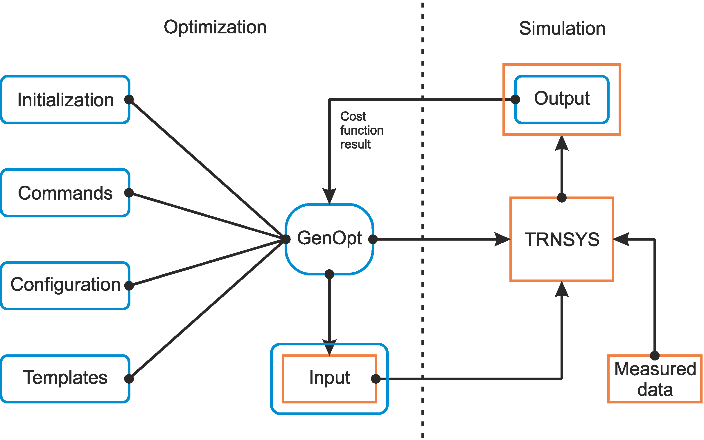Figure 8 shows the architecture and the logic diagram established between GenOpt and Trnsys.

Through this relationship, GenOpt iteratively calls Trnsys, and the objective function is calculated as the design parameters are modified.

In this work, the GPS implementation of the Hooke-Jeeves algorithm is used to minimize the root mean square error (RMSE) of the objective function. This algorithm is a hybrid global optimization algorithm in which a pattern search optimization is combined with the constrictions established by the Hooke-Jeeves algorithm. This method first runs an arbitrary search and then constrains the results using the Hooke-Jeeves algorithm to obtain better accuracy within the results. This hybrid algorithm reaches the global minimum faster than other available algorithms because during the first arbitrary search, it approximates the solution more quickly.

Figure 8. The linking scheme for GenOpt and Trnsys.

Figure 8. The linking scheme for GenOpt and Trnsys.

Cost Function

Equation (11) represents the RMSE equation selected as the objective function to minimize within the GenOpt software:

$$RMSE=\sqrt{\frac{1}{n}·{\displaystyle \sum }_{i=1}^n{\left(T_{sim}-T_{exp}\right)}^2}$$

(11)

In Equation (11), T_sim represents the simulated temperatures, and T_exp is the experimental temperature measured at the SE unit. A similar expression is used to evaluate the error in the produced power. The coefficient of variation of the RMSE, commonly known as CV(RMSE) (12), is defined as the normalized value of the RMSE:

$$CV(RMSE)=\frac{RMSE}{\left|{\overline{T}}_{exp}\right|}$$

(12)

The total error (13) is calculated as the sum of CV(RMSE) for the water outlet temperature, exhaust gases temperature, and power.

$$TOTAL ERROR= \text{CV}{\left(\text{RMSE}\right)}_{Tout}+\text{CV}{\left(\text{RMSE}\right)}_{Texh}+\text{CV}{\left(\text{RMSE}\right)}_{Power}$$

(13)

Thus, combining the GenOpt software with the Trnsys simulation software, the different capacitance values and transfer coefficients that best fit the experimental data while minimizing the TOTAL ERROR are obtained.

The mean bias error MBE is calculated using Equation (14):

$$MBE=\frac{{\displaystyle \sum }\left(T_{sim}-T_{exp}\right)}{n}$$

(14)

7. Results and Discussion

The simulations were conducted using three different block set point temperatures: 45 °C, 60 °C, and 70 °C. First, the optimization was performed independently for these three cases, yielding different values for the capacitances and coefficients of transference.

Table 1 (first three columns) shows the parameter values for the lumped capacitance and heat transfer coefficients for the three set temperatures. All the values show good agreement. Although these values have a physical interpretation, they are not meant to be equal to the actual values. They are simply the values that minimize the cost function. The difference between the first three columns in Table 1 depends on factors such as the time step, the length of the experiment, or errors in the data acquisition. Thus, the third experiment has values similar to the previous ones, except for MC_Block, which is significantly higher. This could be explained by the fact that the third experiment was 30 min shorter than the others and therefore the SE did not spend as long at steady state as it did in the other two experiments.

Table 1. Values of MC_Block, MC_burner, (U·A)_b-b, and (U·A)_HE after model calibration for the three T_set temperatures. Values of MC_Block, MC_burner, (U·A)_b-b, and (U·A)_HE after model calibration for the three simultaneous T_{set, 3T} temperatures.

Parameter	Tset = 45 °C	Tset = 60 °C	Tset = 70 °C	Tset, 3T
$M{C}_{Block}$ (kJ/K)	62.69	61.68	119.94	94.00
$M{C}_{Burner}$ (kJ/K)	12.75	12.94	13.69	12.88
(U·A)b-b (W/K)	10.49	10.64	10.33	38.25
(U·A)HE (W/K)	19.05	19.77	18.91	69.56

Table 1. Values of MC_Block, MC_burner, (U·A)_b-b, and (U·A)_HE after model calibration for the three T_set temperatures. Values of MC_Block, MC_burner, (U·A)_b-b, and (U·A)_HE after model calibration for the three simultaneous T_{set, 3T} temperatures.

Parameter	Tset = 45 °C	Tset = 60 °C	Tset = 70 °C	Tset, 3T
$M{C}_{Block}$ (kJ/K)	62.69	61.68	119.94	94.00
$M{C}_{Burner}$ (kJ/K)	12.75	12.94	13.69	12.88
(U·A)b-b (W/K)	10.49	10.64	10.33	38.25
(U·A)HE (W/K)	19.05	19.77	18.91	69.56

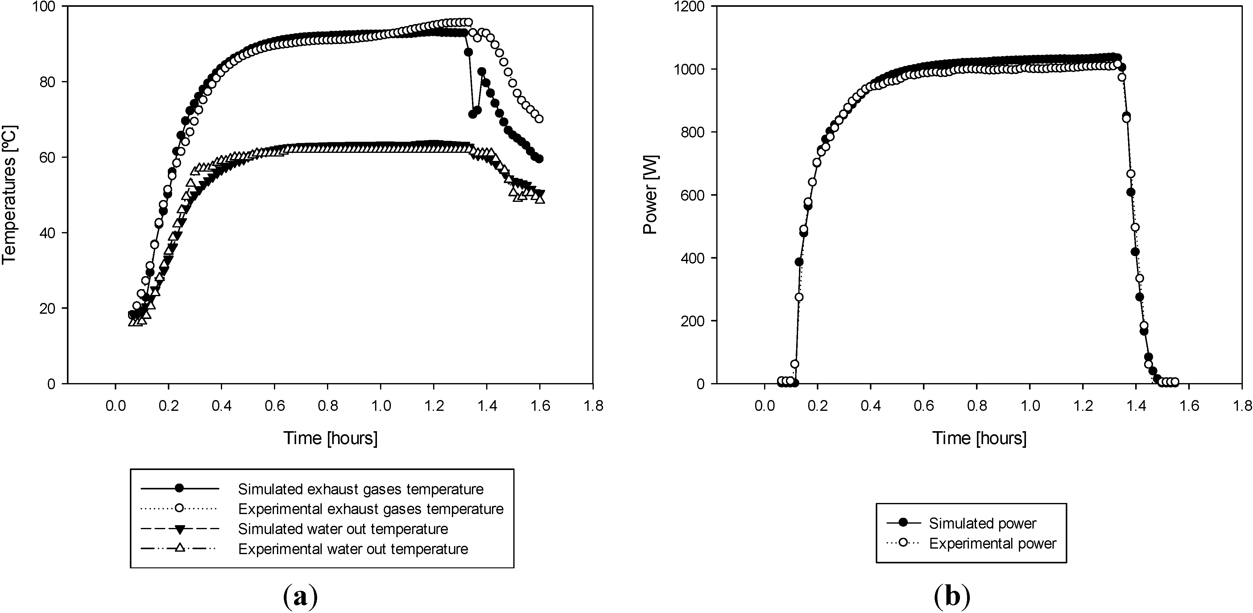
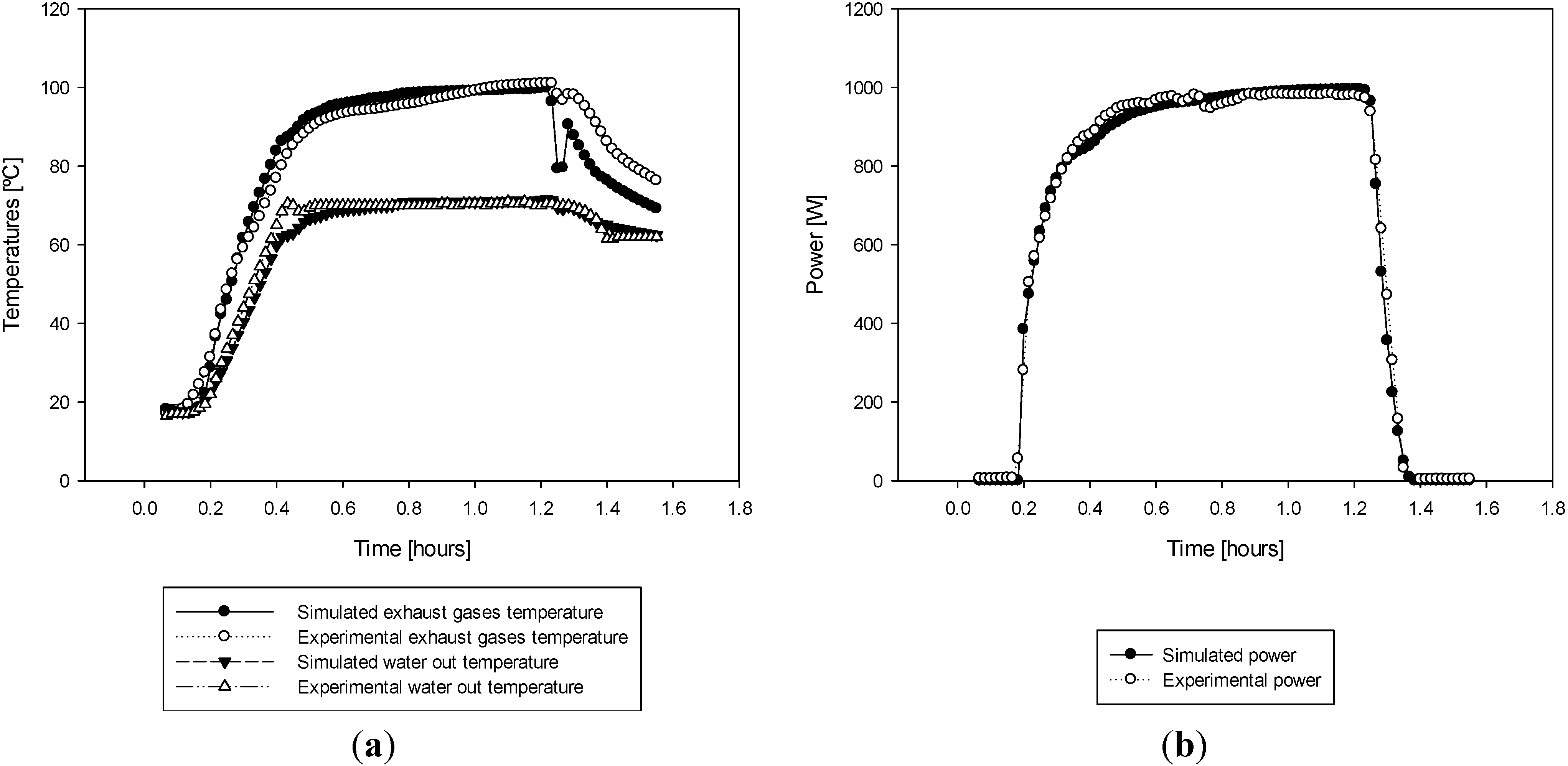
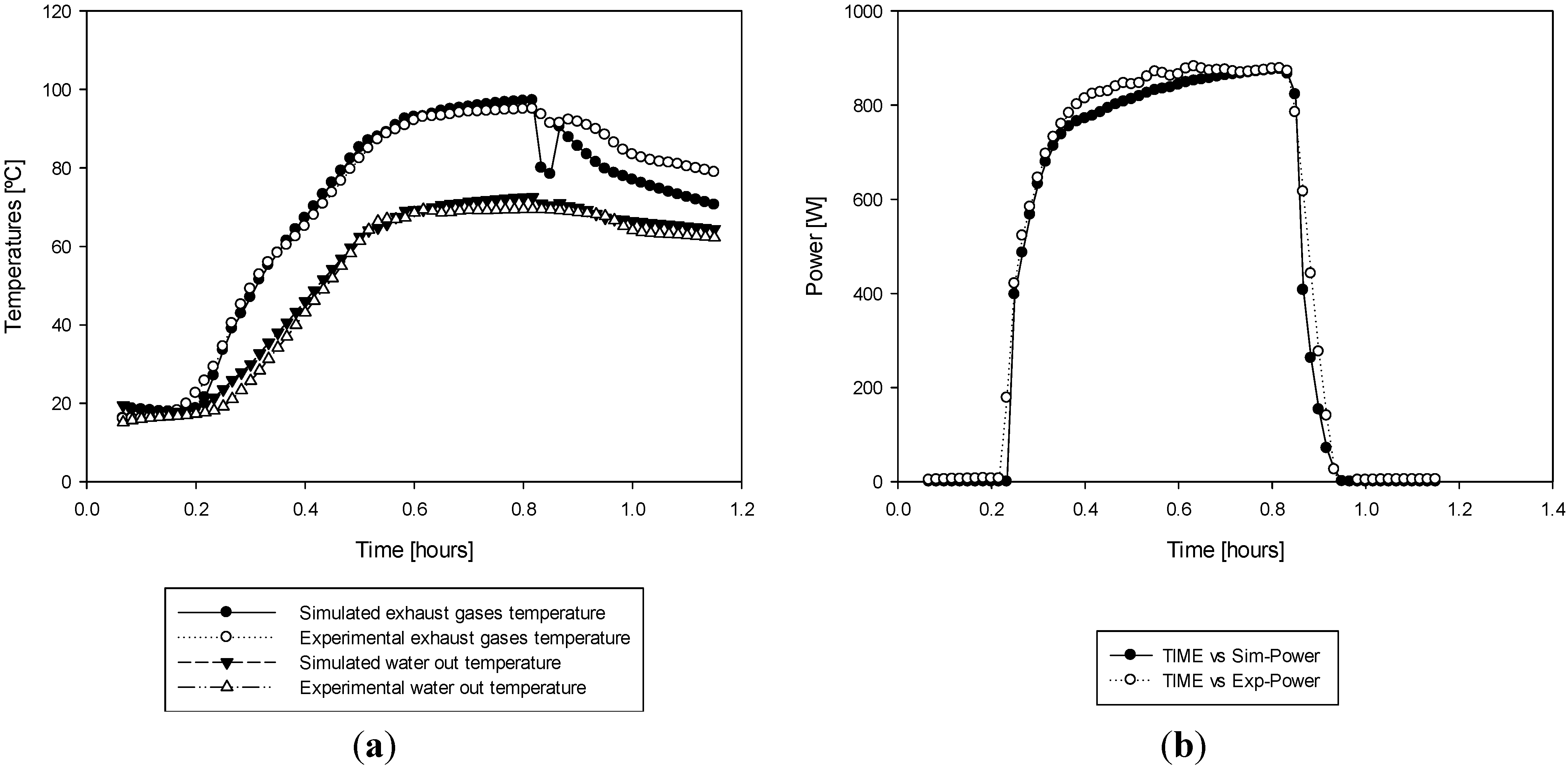
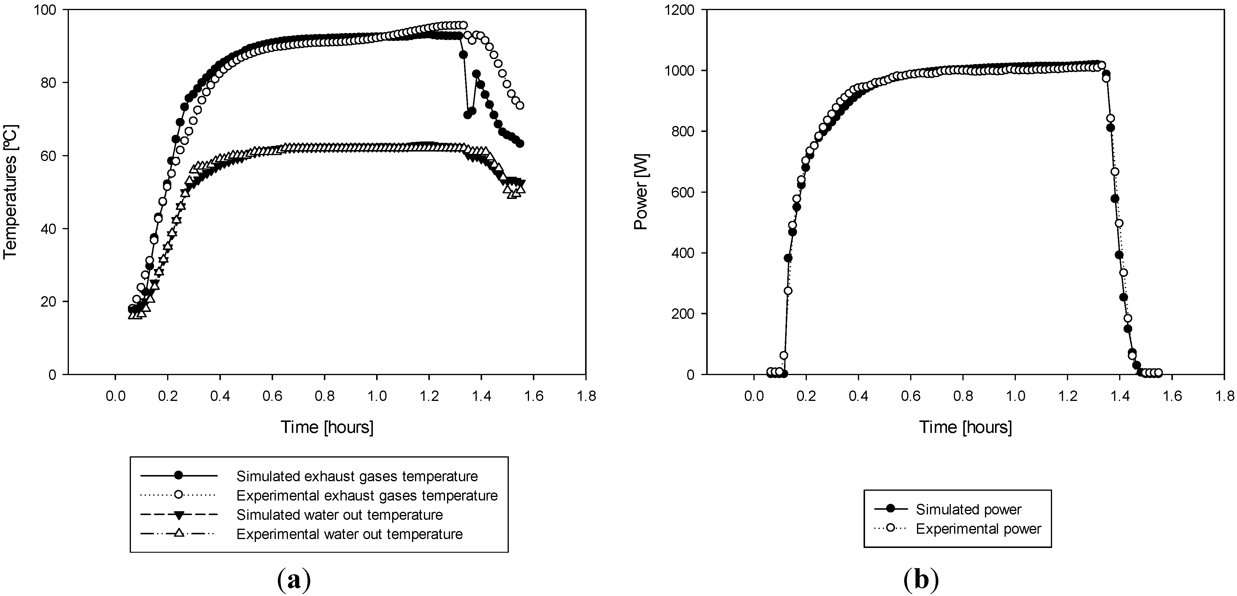
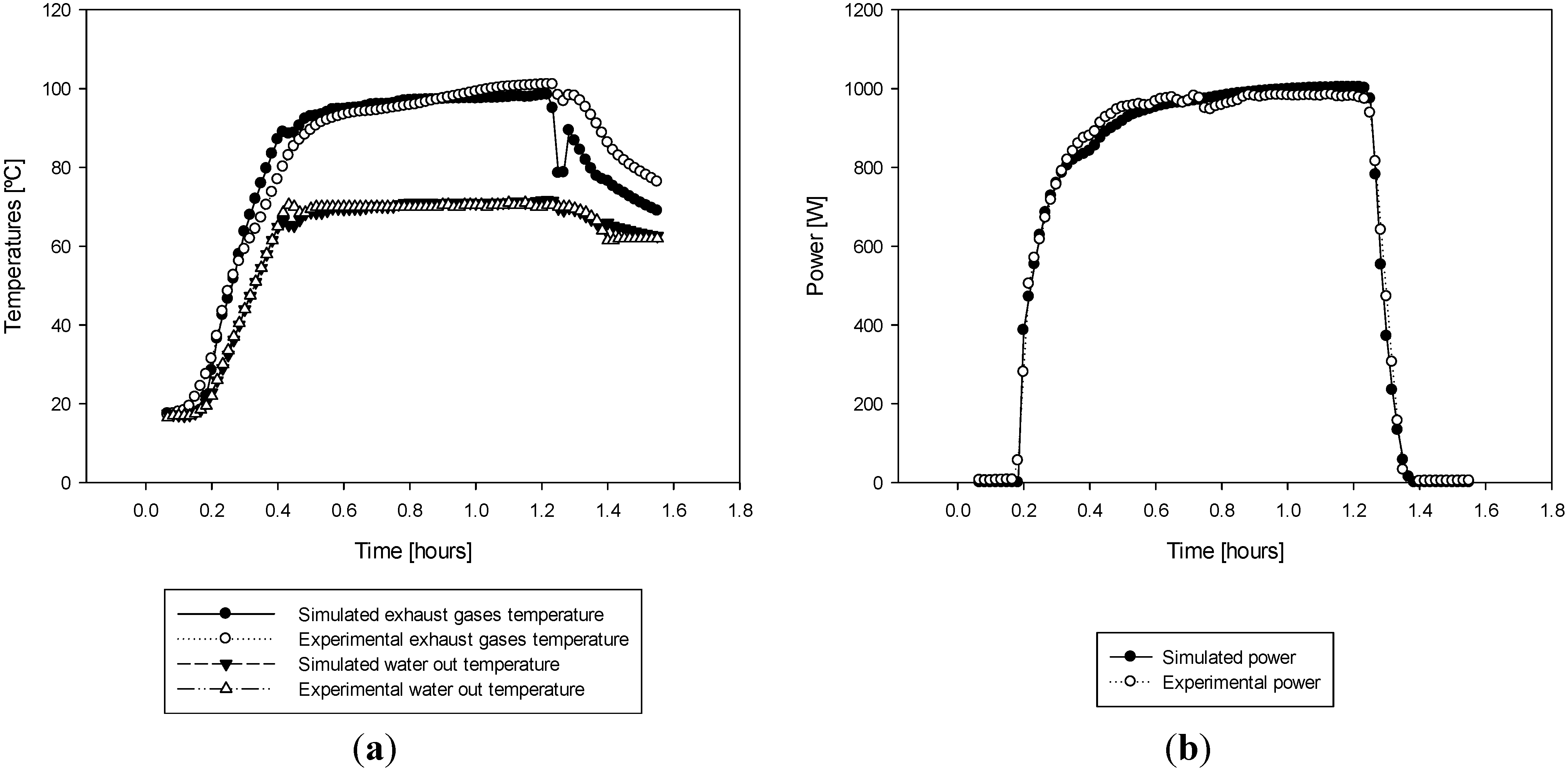
Figure 9a, Figure 10a and Figure 11a show the simulated and experimental data for the exhaust gases temperature and water output temperature. It is shown that the proposed model follows the experimental data. In mode 4, the SE stops the air supply for 30 seconds, which causes the Trnsys model to experience a sudden drop in temperature due to the null capacitance of the heat exchanger model. This behavior is reflected in all graphs and explains why the rest of the values of the simulated temperatures in modes 4 and 5 are less than the logged data. To avoid this sudden dip, a possible improvement in the model could be to add a third lump to provide thermal inertia to the shell and heat exchanger.

The water outlet temperature better matches the real data because there was no stop in the water flow. Additionally, Figure 9b, Figure 10b and Figure 11b show the simulated and experimental power generated. The concordance is even greater.

Table 2 summarizes the errors. The third experiment shows higher values for both RMSE and MBE because this experiment was 30 min shorter and steady state had not yet been reached.

Another optimization process was performed by summing the errors of the simulations for the three temperature set points to validate the lumped capacitance model for all three data sets. Table 1 (last column) provides the results of this optimization. Comparing these values with those given by Table 1, there is a significant variation in the two values of UA, although they have the same order of magnitude.

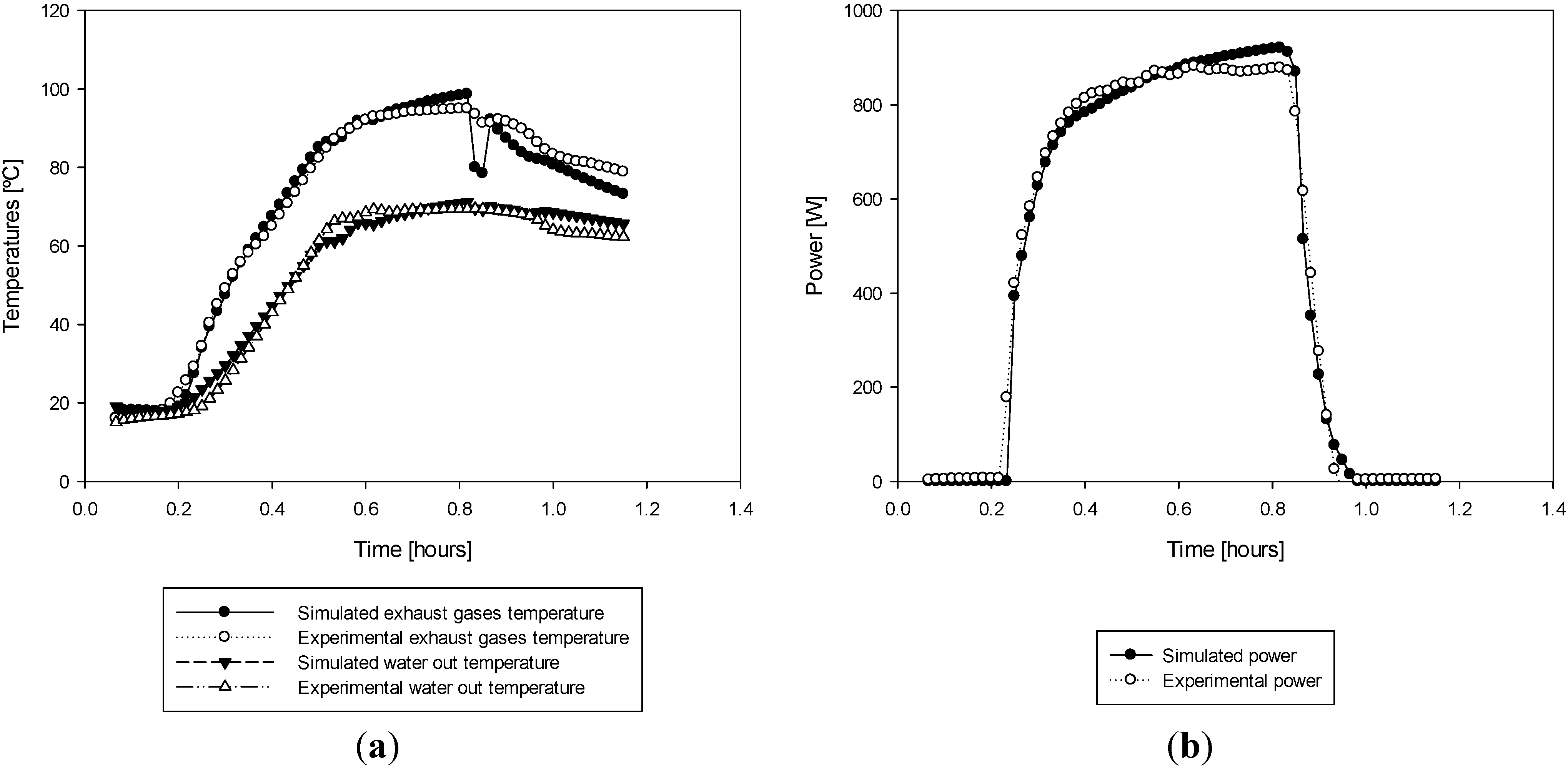
As shown in Figure 12, Figure 13 and Figure 14, the results are still valid. The errors given in Table 3 are higher than those given in Table 2, but the percentage error confirms that the simulations provide the correct values. Indeed, for a set point temperature of 60 °C, the RMSE is 3.56% for the power and 0.45% for the MBE, whereas for the other temperatures, these values are higher but still permissible errors in the energy simulations. Thus, the model is valid for transient simulations without the need to optimize the values of the capacitance and heat transfer coefficients for each operating point. The usefulness and versatility of this solution is demonstrated by the obtained results.

Figure 9. (a) Simulated and experimental outlet water temperature and exhaust gases temperature for T_set = 45 °C; (b) Simulated and experimental power for T_set = 45 °C.

Figure 9. (a) Simulated and experimental outlet water temperature and exhaust gases temperature for T_set = 45 °C; (b) Simulated and experimental power for T_set = 45 °C.

Figure 10. (a) Simulated and experimental outlet water temperature and exhaust gases temperature for T_set = 60 °C; (b) Simulated and experimental power for T_set = 60 °C.

Figure 10. (a) Simulated and experimental outlet water temperature and exhaust gases temperature for T_set = 60 °C; (b) Simulated and experimental power for T_set = 60 °C.

Figure 11. (a) Simulated and experimental outlet water temperature and exhaust gases temperature for T_set = 70 °C; (b) Simulated and experimental power for T_set = 70 °C.

Figure 11. (a) Simulated and experimental outlet water temperature and exhaust gases temperature for T_set = 70 °C; (b) Simulated and experimental power for T_set = 70 °C.

Figure 12. (a) Simulated and experimental outlet water temperature and exhaust gases temperature for T_set = 45 °C; (b) Simulated and experimental power for T_set = 45 °C. The capacitance and heat transfer coefficient values are given in Table 1 (last column).

Figure 12. (a) Simulated and experimental outlet water temperature and exhaust gases temperature for T_set = 45 °C; (b) Simulated and experimental power for T_set = 45 °C. The capacitance and heat transfer coefficient values are given in Table 1 (last column).

Figure 13. (a) Simulated and experimental outlet water temperature and exhaust gases temperature for T_set = 60 °C; (b) Simulated and experimental power for T_set = 60 °C. The capacitance and heat transfer coefficient values are given in Table 1 (last column).

Figure 13. (a) Simulated and experimental outlet water temperature and exhaust gases temperature for T_set = 60 °C; (b) Simulated and experimental power for T_set = 60 °C. The capacitance and heat transfer coefficient values are given in Table 1 (last column).

Figure 14. (a) Simulated and experimental outlet water temperature and exhaust gases temperature for T_set = 70 °C; (b) Simulated and experimental power for T_set = 70 °C. The capacitance and heat transfer coefficient values are given in Table 1 (last column).

Figure 14. (a) Simulated and experimental outlet water temperature and exhaust gases temperature for T_set = 70 °C; (b) Simulated and experimental power for T_set = 70 °C. The capacitance and heat transfer coefficient values are given in Table 1 (last column).

Table 2. Values of CV(RMSE) and MBE for T_exh, T_out, and Power for the three T_set temperatures.

Type of error	Tset = 45 °C	Tset = 60 °C	Tset = 70 °C
CV(RMSE) tgas	7.33%	6.94%	4.34%
MBE tgas	−0.93 (1.18%)	−1.16 (1.47%)	−0.85 (1.26%)
CV(RMSE) twater_out	2.31%	2.35%	5.71%
MBE twater_out	0.13 (0.23%)	0.25 (0.42%)	1.23 (2.49%)
CV(RMSE) power	2.88%	3.87%	7.39%
MBE power	−0.98 (0.13%)	−0.67 (0.10%)	−4.48 (0.99%)

Table 2. Values of CV(RMSE) and MBE for T_exh, T_out, and Power for the three T_set temperatures.

Type of error	Tset = 45 °C	Tset = 60 °C	Tset = 70 °C
CV(RMSE) tgas	7.33%	6.94%	4.34%
MBE tgas	−0.93 (1.18%)	−1.16 (1.47%)	−0.85 (1.26%)
CV(RMSE) twater_out	2.31%	2.35%	5.71%
MBE twater_out	0.13 (0.23%)	0.25 (0.42%)	1.23 (2.49%)
CV(RMSE) power	2.88%	3.87%	7.39%
MBE power	−0.98 (0.13%)	−0.67 (0.10%)	−4.48 (0.99%)

Table 3. Values of CV(RMSE) and MBE for T_exh, T_out, and Power for the three T_{set, 3T} temperatures.

Type of error	Tset = 45 °C	Tset = 60 °C	Tset = 70 °C
CV(RMSE) tgas	6.78%	6.32%	6.43%
MBE tgas	−1.39 (1.76%)	−0.71 (0.90%)	−1.79 (2.65%)
CV(RMSE) twater_out	3.55%	4.10%	4.99%
MBE twater_out	0.20 (2.57%)	−0.68 (1.16%)	2.05 (4.13%)
CV(RMSE) power	3.57%	3.56%	8.30%
MBE power	16.06 (2.16%)	−2.85 (0.45%)	−22.23 (4.93%)

Table 3. Values of CV(RMSE) and MBE for T_exh, T_out, and Power for the three T_{set, 3T} temperatures.

Type of error	Tset = 45 °C	Tset = 60 °C	Tset = 70 °C
CV(RMSE) tgas	6.78%	6.32%	6.43%
MBE tgas	−1.39 (1.76%)	−0.71 (0.90%)	−1.79 (2.65%)
CV(RMSE) twater_out	3.55%	4.10%	4.99%
MBE twater_out	0.20 (2.57%)	−0.68 (1.16%)	2.05 (4.13%)
CV(RMSE) power	3.57%	3.56%	8.30%
MBE power	16.06 (2.16%)	−2.85 (0.45%)	−22.23 (4.93%)

8. Conclusions

This article proposes a dynamic model of an SE with 0.92 kW of electric power and 6 kW of thermal power. This model is based on two lumps and a heat exchanger. Using these components, a series of simulations were conducted in Trnsys, and the validity of the model was evaluated by comparing the experimentally obtained data with the data obtained from the simulation. Furthermore, the model calibration was performed using GenOpt, reducing the RMSE through the variation of basic parameters from the model.

The model was shown to faithfully reflect reality, with errors on the order of 1% or less, and it was also proven to predict the behavior of an SE under steady state and to follow the start-up and shutdown curves. This model is applicable to Whispergen DC PPS16-24MD personal power station, but it could be extended to other SEs, which would require a new calculation of MC_Block, MC_burner capacitances, and the overall heat transfer coefficients (U·A)_b-b and (U·A)_HE. These results indicate that the MC_Block value is approximately eight times the value of MC_burner, which explains the quick drop in the temperature of the exhaust gases compared with the drop in water temperature output once the SE has been powered off.

Based on the system results and by analyzing the geometry of the SE, it has been demonstrated that during start-up and steady state, the system power is directly proportional to the temperature difference between the burner and the block.

The simulated electrical power output also fits the experimental logged data, demonstrating that this model is appropriate for dynamic simulations because all the important outputs are well generated. In this way, the obtained model can be introduced directly in a simulation environment to explore its application in different buildings or locations throughout an entire year, taking into account the different transient responses. Finally, a calibration using three dataset values was performed to provide a model that would be valid across the range of outlet water temperatures. Using these parameters, the simulation also provided acceptable results.

Future works will analyze the behavior of this micro-CHP system at different operating points, modifying the T_burner set point and air supply conditions to analyze the performance and the variations in the efficiency of the SE cogeneration device.