Harmonic Propagation and Interaction Evaluation between Small-Scale Wind Farms and Nonlinear Loads

Abstract

Distributed generation is a flexible and effective way to utilize renewable energy. The dispersed generators are quite close to the load, and pose some power quality problems such as harmonic current emissions. This paper focuses on the harmonic propagation and interaction between a small-scale wind farm and nonlinear loads in the distribution grid. Firstly, by setting the wind turbines as P – Q(V) nodes, the paper discusses the expanding Newton-Raphson power flow method for the wind farm. Then the generalized gamma mixture models are proposed to study the non-characteristic harmonic propagation of the wind farm, which are based on Gaussian mixture models, improved phasor clustering and generalized Gamma models. After the integration of the small-scale wind farm, harmonic emissions of nonlinear loads will become random and fluctuating due to the non-stationary wind power. Furthermore, in this paper the harmonic coupled admittance matrix model of nonlinear loads combined with a wind farm is deduced by rigorous formulas. Then the harmonic propagation and interaction between a real wind farm and nonlinear loads are analyzed by the harmonic coupled admittance matrix and generalized gamma mixture models. Finally, the proposed models and methods are verified through the corresponding simulation models in MATLAB/SIMULINK and PSCAD/EMTDC.

1. Introduction

Following the depletion of fossil energy, renewable energy generation is a fast growing area nowadays. With the increasing installed wind power generation capacity, we need to find more effective ways to utilize wind energy.

Different for large-scale wind farms integrated into the regular high voltage transmission line [1,2], dispersed wind generators are more flexible. Small-scale wind farms usually consist of several dispersed wind generators, which are directly connected to a medium or low voltage distribution grid [3]. This allows the effective utilization of the limited wind resource in cities or suburbs and shortens the transmission distance. The small-scale wind farm is however quite close to the load, which can pose some power quality problems such as voltage fluctuation and harmonic current emissions.

The system impedance in the distribution grid is highly resistive, and the voltage fluctuation at the Point of Common Coupling (PCC) is strongly affected by wind power smoothing level [4,5]. Wind power data are non-stationary random signals because of the variable wind speed and wind energy conversion systems [6,7,8]. At the same time, the fluctuating fundamental power can affect the controller of conversion systems and induce harmonics, so the harmonic current emissions of wind generators are analyzed by stochastic assessment. New models and methods for harmonic propagation and interaction issues can be verified in several simulation systems, such as MATLAB/SIMULINK, PSCAD/EMTDC and HYPERSIM [9,10,11].

Harmonic current emissions of wind generators consist of characteristic and non-characteristic harmonics. Characteristic harmonics are affected by the topology structure of converters and the switch control strategy of converter valves, whereas non-characteristic harmonics are induced by the inherent slot harmonics of wind turbines, nonsinusoidal distributions of the stator and rotor windings, and operating conditions of converters and the outside power grids [12,13]. Non-characteristic harmonics of different wind turbines are almost independent low-order harmonics, even for the doubly fed induction generator and direct-drive permanent magnet generator.

In order to analyze the complex harmonic current emissions, Generalized Gamma Mixture Models (GGMM) are proposed in this paper. GGMM consists of Gaussian mixture models, improved phasor clustering and generalized Gamma models. GGMM divide the complicated probability distribution functions (pdfs) of harmonic sources for the harmonic propagation and interaction study. On the other hand, the port characteristics of nonlinear devices in the distribution gird become variable due to the installed wind generation. Power electronic devices are normally nonlinear [14,15], and the AC/DC converter is important for them. The DC side part can be a linear load, battery, and motor drives with DC/AC inverters [16,17]. These nonlinear loads generate several kinds of harmonic emissions into the power grid, and iterative harmonic analysis is the common way to study harmonic power flow [18]. In order to analyze the harmonic power flow, accurate harmonic source modeling is necessary. The predetermined and harmonic–voltage dependent current source models are both defective [14,18]. Reference [15] proposes a harmonic admittance matrix to reflect the relationship between the AC side harmonic voltages and currents of a rectifier. The harmonic coupled admittance matrix model is strictly deduced and adjusted for the harmonic interaction in this paper.

Therefore this paper focuses on the harmonic propagation and interaction between a small-scale wind farm and nonlinear loads in the distribution grid. Harmonic emissions of nonlinear loads become random and fluctuant due to the non-stationary wind power, meanwhile wind harmonic emissions make it more complex. In this paper, first the power flow expanding model of wind turbines based on P − Q(V) characteristic is studied, and GGMM of harmonic current are proposed and described in detail. The switching harmonic currents produced by the grid-side and rotor-side converters of are also analyzed in depth. Then the harmonic admittance matrix models of nonlinear loads combined with the wind farm are established to analyze the harmonic propagation and interactions. Finally, the proposed models and methods are verified through a simulation model in MATLAB/SIMULINK and PSCAD/EMTDC.

2. Power Flow and Harmonic Source Modeling of Wind Farm

2.1. Power Flow Modeling of Wind Farm

When a small-scale wind farm is installed in the distribution grid, the port characteristics of nonlinear loads will become more complex. Compared to the variable loads, the small-scale wind farm induces a fluctuating negative power flow, and supplies voltage to the distribution grid.

The most common forms of wind generation contain asynchronous generators (AGs), doubly-fed induction generators (DFIGs) and direct-drive generators. In this paper, the DFIG is modeled to study the harmonic propagation in the distribution grid. The topological diagram of the small-scale wind farm is shown in Figure 1.

The steady state circuit model of DFIG is shown in Figure 2 [19]. The term ω_e is the nominal angular speed, ω_s, ω_r, ω_m are the stator, rotor, and rotating angular speed, and N = ±1 represents the positive and negative circuit. When the fundamental power flow is studied, ω_s = ω_e, N = 1, $slip=s=\frac{{\omega }_e-{\omega }_m}{{\omega }_e}$.

Figure 1. The topological diagram of the small-scale wind farm.

Figure 1. The topological diagram of the small-scale wind farm.

Figure 2. The steady state circuit model of DFIG.

Figure 2. The steady state circuit model of DFIG.

The reactive power of DFIG is affected by the bus voltage, which is different from the normal PQ or PV node in the power flow study, so the expanding Newton-Raphson power flow method is utilized to study the fundamental power flow, in which the wind generations are set as P − Q(V) nodes [20,21]. The Q − V relationship is given by Equation (1), and the output active power is affected by wind speed:

(1)

where X_ss = X_s + X_m; $a=\frac{r_r^{\prime }{X}_{ss}^2}{X_m^2{\text{sin}}^2\phi }$; $b=\frac{2r_r^{\prime }{X}_{ss}}{X_m^2}+\frac{1-s}{\text{tan }\phi }$; $c=\frac{r_r^{\prime }}{X_m^2}$; d = P; cos φ is the power factor, ${\dot{V}}_s$ represents the stator voltage; ${\dot{I}}_s$ represents the stator current; ${\dot{V}}_r^{\prime }$ represents the rotator voltage; ${\dot{I}}_r$ represents the rotator current; r_s and X_s represent the stator resistance and reactance respectively; $r_r^{\prime }$ and X_r represent the rotator resistance and reactance respectively; X_m is the excitation reactance; slip = s is the slip ratio.

Define P_is as the active power, P − Q(V) nodes are used to represent the wind power nodes, and their corresponding power equations in the expanding Newton-Raphson models are given by Equation (2):

(2)

where:

2.2. Harmonic Source Modeling of Wind Farm

In order to analyze the harmonic emissions of DFIG more accurately, a detailed model is established in MATLAB/SIMULINK. The back to back converter is typically based on a two-level voltage source. The electrical control strategies of the rotor and grid side converters are based on reference [22]. Pulse Width Modulation (PWM) is used to reduce the harmonic emissions and the topological diagram of DFIG is shown in Figure 3.

The harmonic emissions of DFIG mainly consist of three parts: (i) the inherent harmonics; (ii) the switching harmonics; and (iii), the harmonics induced by the unbalance conditions or the background harmonic voltage.

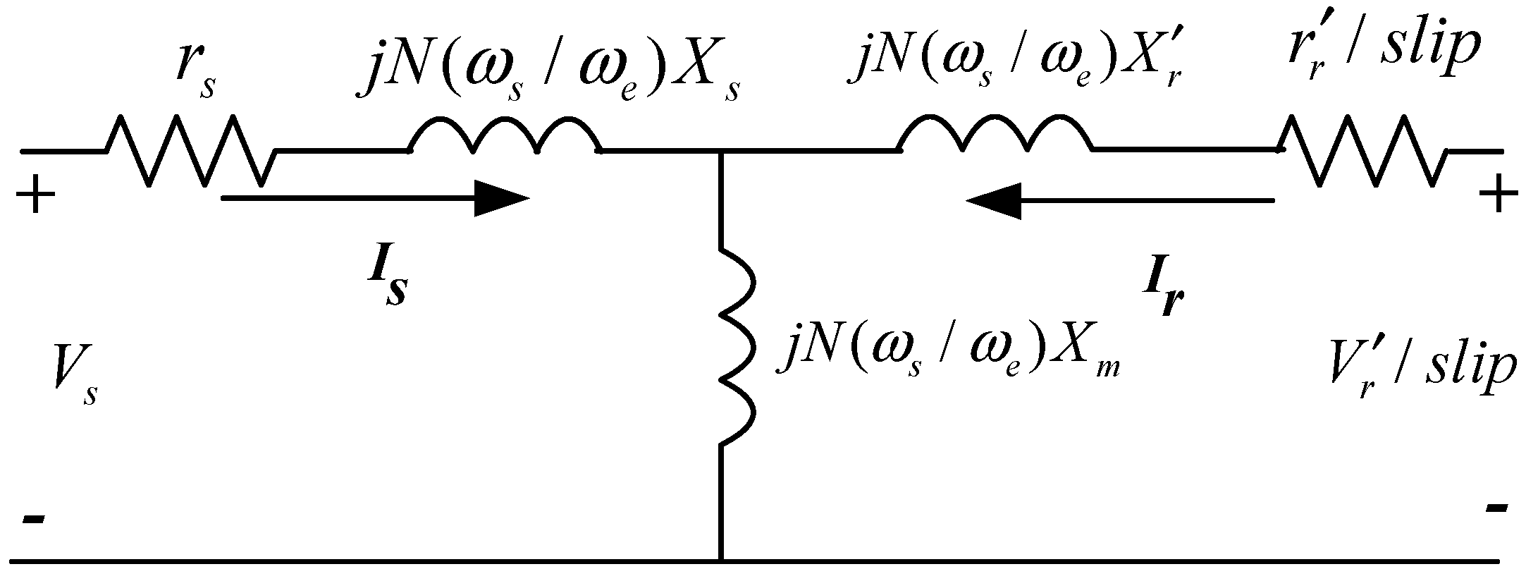
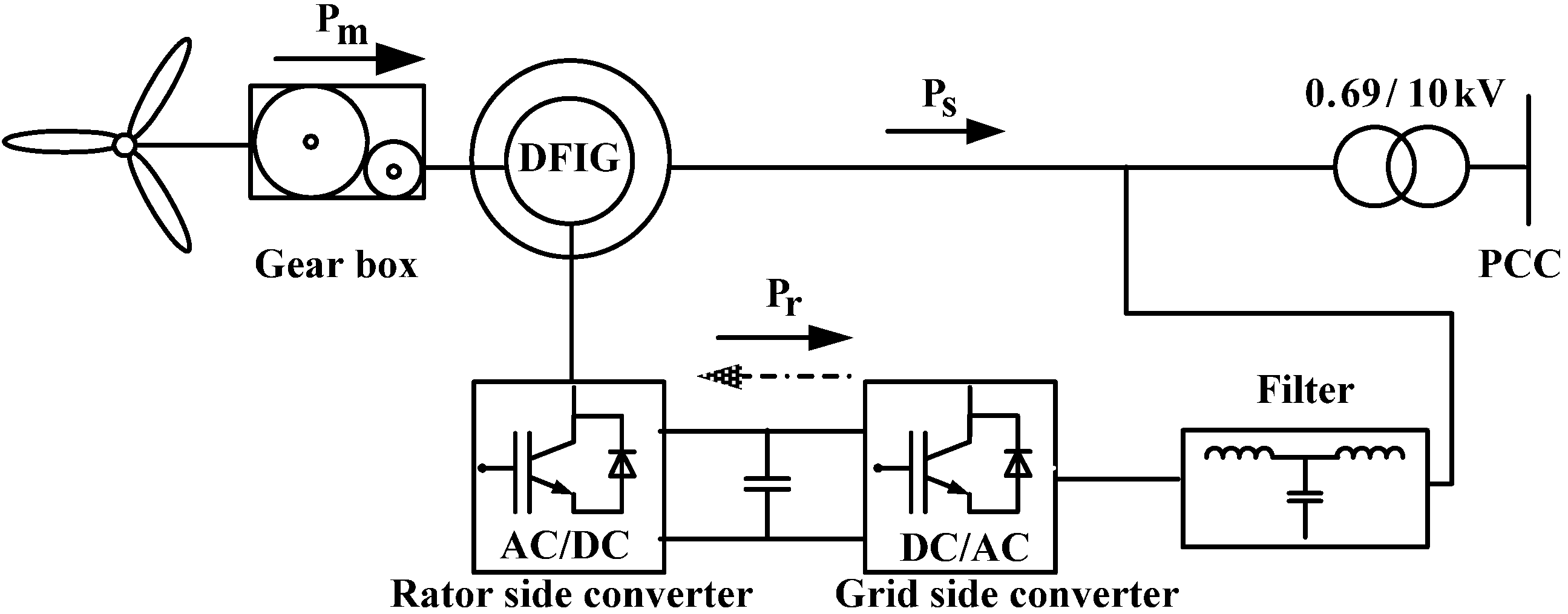
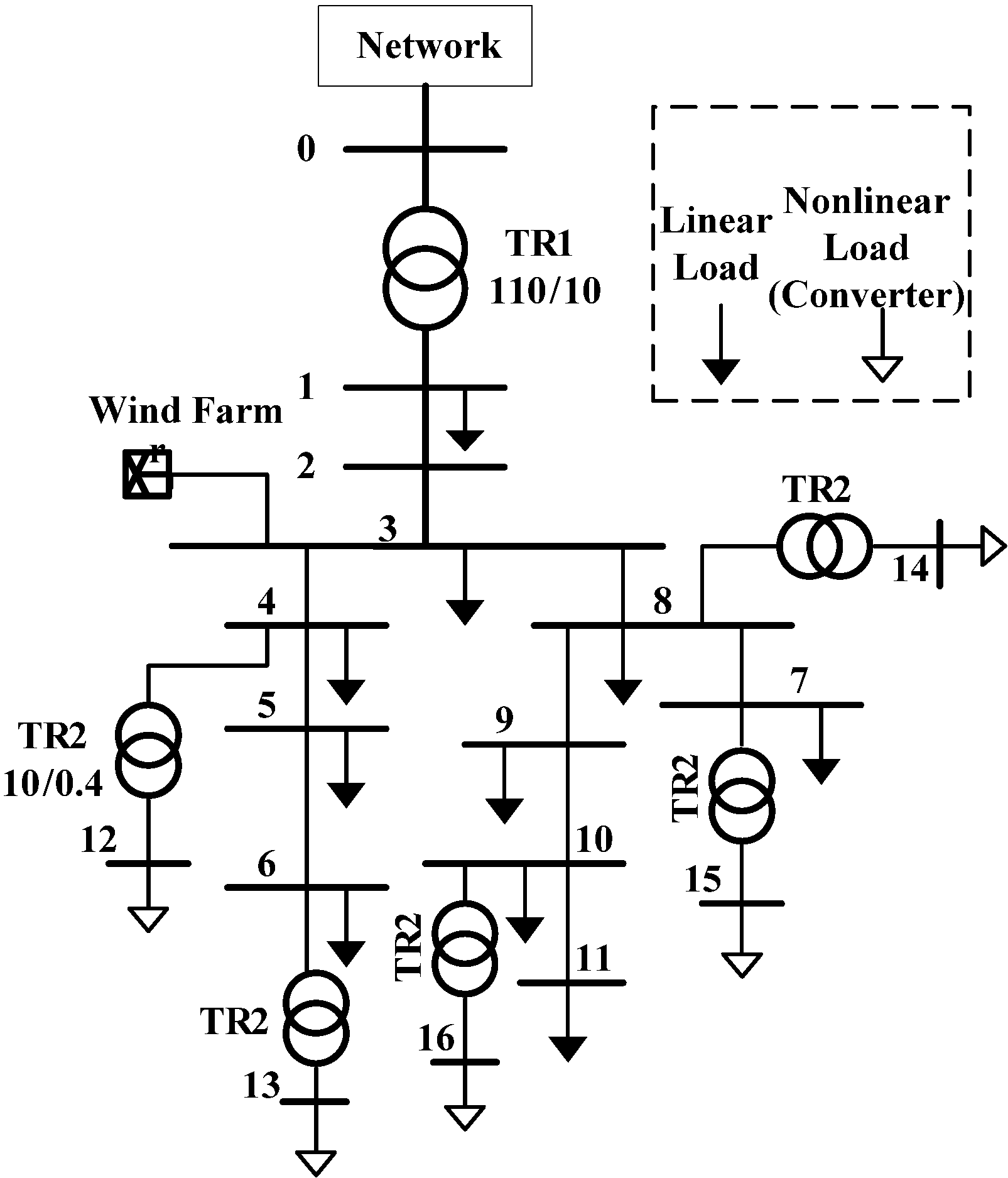
Figure 3. The topological diagram of DFIG.

Figure 3. The topological diagram of DFIG.

The inherent harmonics are from a mechanism such as the induction machine. Slot harmonics produced by variation in the reluctance due to the slots are typical inherent harmonics [23,24]. Nonsinusoidal distributions of the stator and rotor windings generate the Magnetic Motive Force (MMF) space harmonics [11,24,25].

The switching harmonics are produced by the rotor and grid side converters, and different switching strategies and frequencies cause different harmonic emission levels [26,27,28].

The disturbed operation conditions also induce harmonic DFIG emissions, such as the background harmonic voltage, the nonsinusoidal rotor injection, the unbalanced stator load scenario, and the unbalanced grid-connected operation [10,29,30].

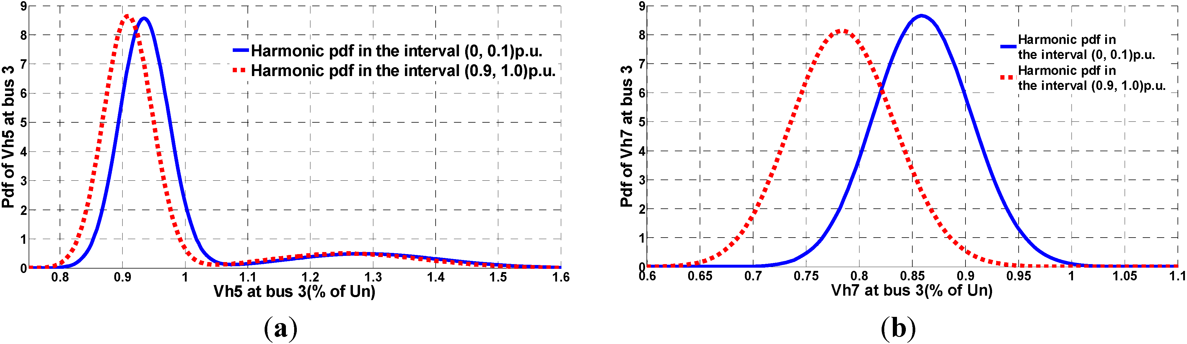
The harmonics emissions named non-characteristic harmonics and caused by nonsinusoidal distribution and disturbed operation conditions, are nonlinear and variable. Papathanassiou, Tentzerakis and Sainz studied the harmonic emissions of practical wind turbines in references [12,13,31], and drew two important conclusions: (i) the influence of a wind farm operating point on harmonic current is small, and the pdfs of h_th harmonic currents do not change significantly from one power level to another; (ii) the fifth and seventh harmonics are the dominant components, and the total harmonic current distortion mainly depends on them, so the low order harmonics are the main components of non-characteristic harmonics. In this paper the fifth and seventh harmonics are researched in depth, and the proposed models are also valid for other low order harmonic emissions. This paper focuses on the evaluation of the non-characteristic and switching harmonic emissions of a small-scale wind farm. The orders of the non-characteristic harmonics are the fifth and seventh, and the order of the switching harmonic is affected by the switching frequency.

2.2.1. Low Order Non-Characteristic Harmonics

When the fifth harmonic current is analyzed, the steady state circuit of DFIG is in negative sequence. The parameters in Figure 2 are calculated as follows: N = −1, ω_s = 5ω_e, f_s = 5f_e, f_r = f_s + f_m = 5f_e + (1 − s)f_e = (6 − s)f_e, $slip=\frac{f_s+f_m}{f_s}=\frac{6-s}{5}$.

When the seventh harmonic current is analyzed, the steady state circuit of DFIG is in positive sequence. The parameters in Figure 2 are calculated as follows: N = 1, ω_s = 7ω_e, f_s = 7f_e, f_r = f_s − f_m = 7f_e − (1 − s)f_e = (6 + s)f_e, $slip=\frac{f_s+f_m}{f_s}=\frac{6+s}{5}$.

s = (f_e − f_m)/f_e > 0 represents sub-synchronous operating status; s = (f_e − f_m) / f_e < 0 represents super-synchronous operating status.

Due to the stochastic and variable non-characteristic harmonic emissions, the probability methodology is utilized. ${\overline{I}}_h=I_h\angle {\varphi }_h=X_h+j{Y}_h$ is set as a random harmonic phasor. If the pdfs of X_h and Y_h can be approximated by Gaussian distributions, the joint probability distribution functions of X_h and Y_h will agree with Equation (3):

(3)

where: , r_XhYh is the correlation coefficient of X_h and Y_h, μ_Xh and μ_Yh are the mean values, σ_Xh and σ_Yh are the standard deviation values.

The pdfs of I_h and ϕ_h are given by Equation (4):

(4)

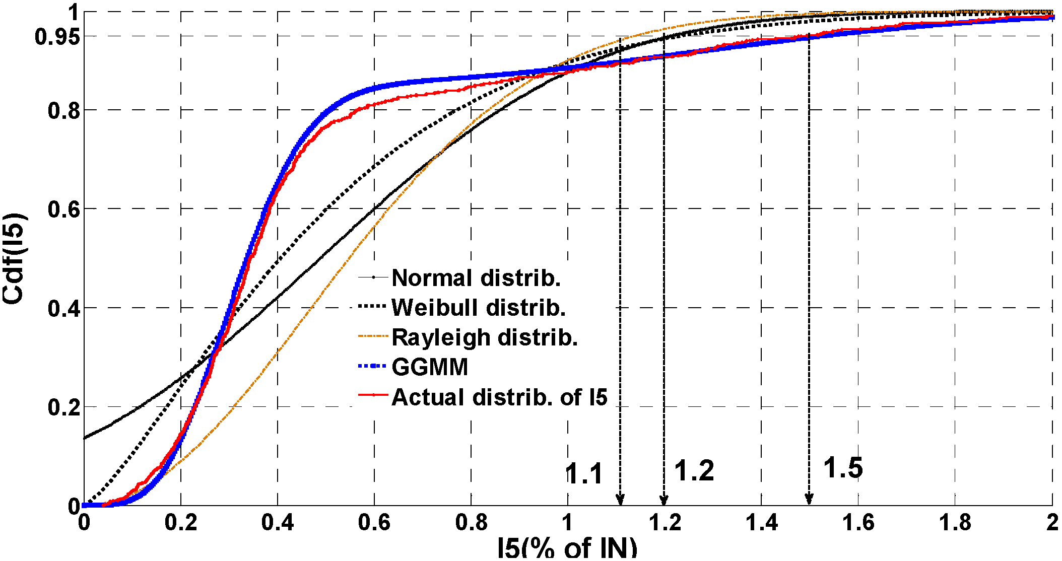
Traditional Rayleigh distribution, Bessel function, and Rician distribution are all derived from Equation (4), in the hypothesis that the pdfs of X_h and Y_h can be approximated by Gaussian distributions [32]. The hypothesis is important to study the harmonic propagation and summation [33].

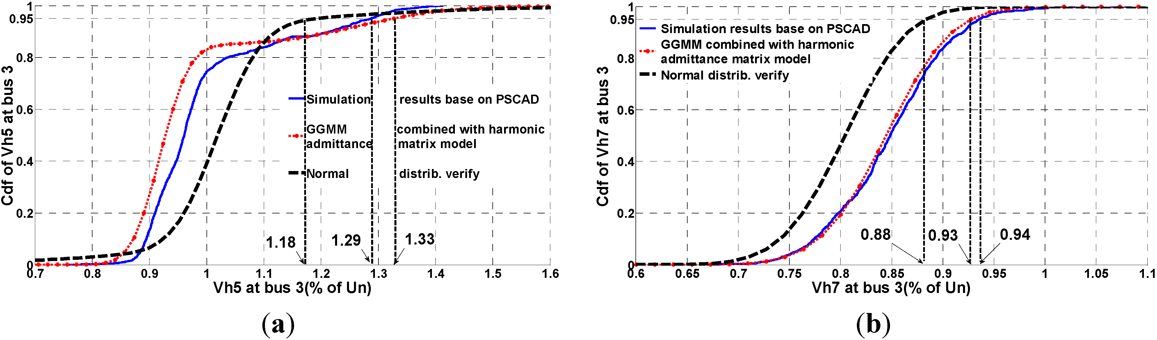
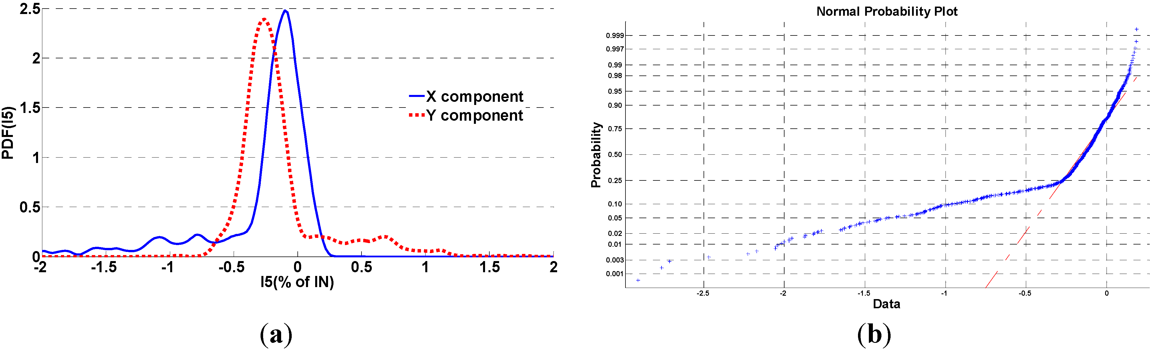
For a large-scale wind farm, the number of wind power generators is large enough to ensure the Gaussian hypotheses of X_h and Y_h based on the central limit theorem, but for a small-scale wind farm, the number of wind power generators is limited, and the probability distribution of the non-characteristic low order harmonic may not be the normal distribution [13,31].

If the probability distribution function (pdf) of the harmonic emission becomes complex, the harmonic propagation and interaction analysis will be difficult. In this paper, Generalized Gamma Mixture Models are proposed to study the probability distributions of non-characteristic harmonics. And GGMM consist of the Gaussian mixture models, improved phasor clustering and generalized Gamma models.

(i) Gaussian mixture models

Gaussian mixture models (GMMs) can accurately approach the non-negative Riemann integral functions such as different pdfs by dividing the complicated pdfs into several simplified Gaussian distributions [34]. GMMs are fitted with Equation (5):

$$f_M(x)={\displaystyle \sum _{m=1}^M}{\epsilon }_m{\varphi }_m(x)$$

(5)

where: ${\displaystyle \sum _{m=1}^M}{\epsilon }_m=1$; and M is the order of GMM; ε_m is the weighted coefficient; ϕ_m(x) is the m-th Gaussian distribution with mean value μ_m and variance value ${\sigma }_m^2$. $\theta =\{{\epsilon }_1,\dots ,{\epsilon }_M;{\mu }_1,\dots ,{\mu }_M;{\sigma }_1^2,\dots ,{\sigma }_M^2\}$ are the parameters of GMM, and can be estimated by expectation maximization (EM) method [35,36].

(ii) Improved phasor clustering models

After step (i), the pdfs of X_h and Y_h can be divided into several Gaussian components:

(6)

But the pdf of harmonic phasor amplitude is determined by X_h, Y_h and their correlation coefficient. If r_XhYh = 0, the pdf of harmonic phasor amplitude can be given by Equation (7):

(7)

But if r_XhYh ≠ 0, Equation (7) is not adequate. The optimal phasor clustering method which can obtain the inherent characteristic of harmonic phasors is proposed to solve the correlation problem. Reference [3] divides the harmonic phasors based on the shortest distance away from the central phasors. In this paper, the harmonic phasors are clustered by the whole distribution characteristic.

Firstly, the central phasors are defined as (μ_xm, μ_yn) based on Cartesian axes, and their dimension is m × n. μ_xm and μ_yn are the mean values of X_h and Y_h based on step (i).

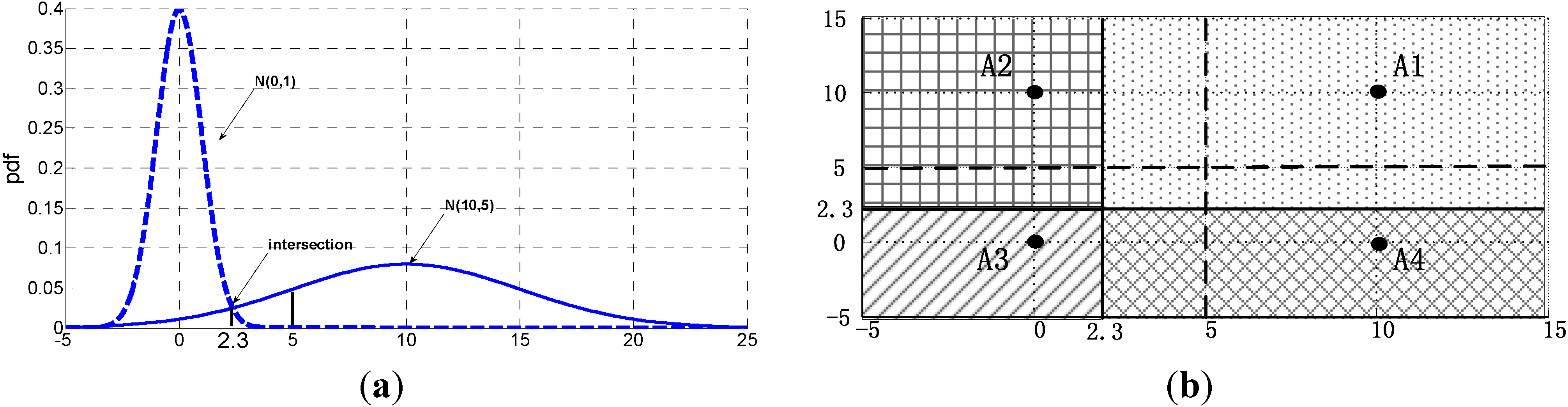
Then the vector space is divided into several regions according to the statistical properties of the Gaussian components in step (i). If the division rule is the shortest distance away from the central phasors, the variance characteristic will be ignored, so the optimal phasor clustering method divides the vector space by the intersection among the Gaussian components.

For example, the pdf of a phasor’s X component is combined by two Gaussian functions, N(0,1) and N(10,5). The intersection point is (2.3, 0.025), as shown in Figure 4a. x = 2.3 is set as the first division axis. The pdf of Y component is just the same, and y = 2.3 is the second division axis. x = 5 and y = 5 are the division axis under the shortest distance rule. The harmonic phasors between x = 2.3 and x= 5 should belong to the N(10,5) part, so the shortest distance rule is not adequate. Furthermore, the divided regions are presented in Figure 4b. The optimal phasor clustering method contains the whole probability property of harmonic phasors.

After phasor clustering, the pdfs of X_h and Y_h in each cluster can be approximated by Gaussian distribution. So if r_XhYh ≠ 0, the pdf of harmonic phasor amplitude based on phasor clustering can be given by Equation (8):

(8)

Figure 4. Verification of the optimal phasor clustering. (a) Pdf and division axis of X component; (b) Comparison of two clustering method.

Figure 4. Verification of the optimal phasor clustering. (a) Pdf and division axis of X component; (b) Comparison of two clustering method.

(iii) Generalized Gamma models

After step (i) and (ii), the pdf of harmonic currents can be given by Equations (7,8). And the complicated pdf is divided into the ideal functions like f_m,n(x + jy) or f_k(x + jy) which can be approximated by GGD due to the pdfs of X_h and Y_h in each cluster agree with Gaussian distributions.

GGD with two parameters is given by Equation (9):

(9)

where: ; $\beta =\sqrt{{\mu }_{X_h}^2+{\mu }_{Y_h}^2+{\sigma }_{X_h}^2+{\sigma }_{Y_h}^2}$; $C=4r_{X_h{Y}_h}{\sigma }_{X_h}^2{\sigma }_{Y_h}^2(2{\mu }_{X_h}{\mu }_{Y_h}+r_{X_h{Y}_h}{\sigma }_{X_h}^2{\sigma }_{Y_h}^2)$.

According to the above three steps, any kind of pdfs of harmonic phasors can be approximated by GGMM. And if the pdfs of X and Y are just fitted with Gaussian distribution, GGMM will be directly modeled by step (iii).

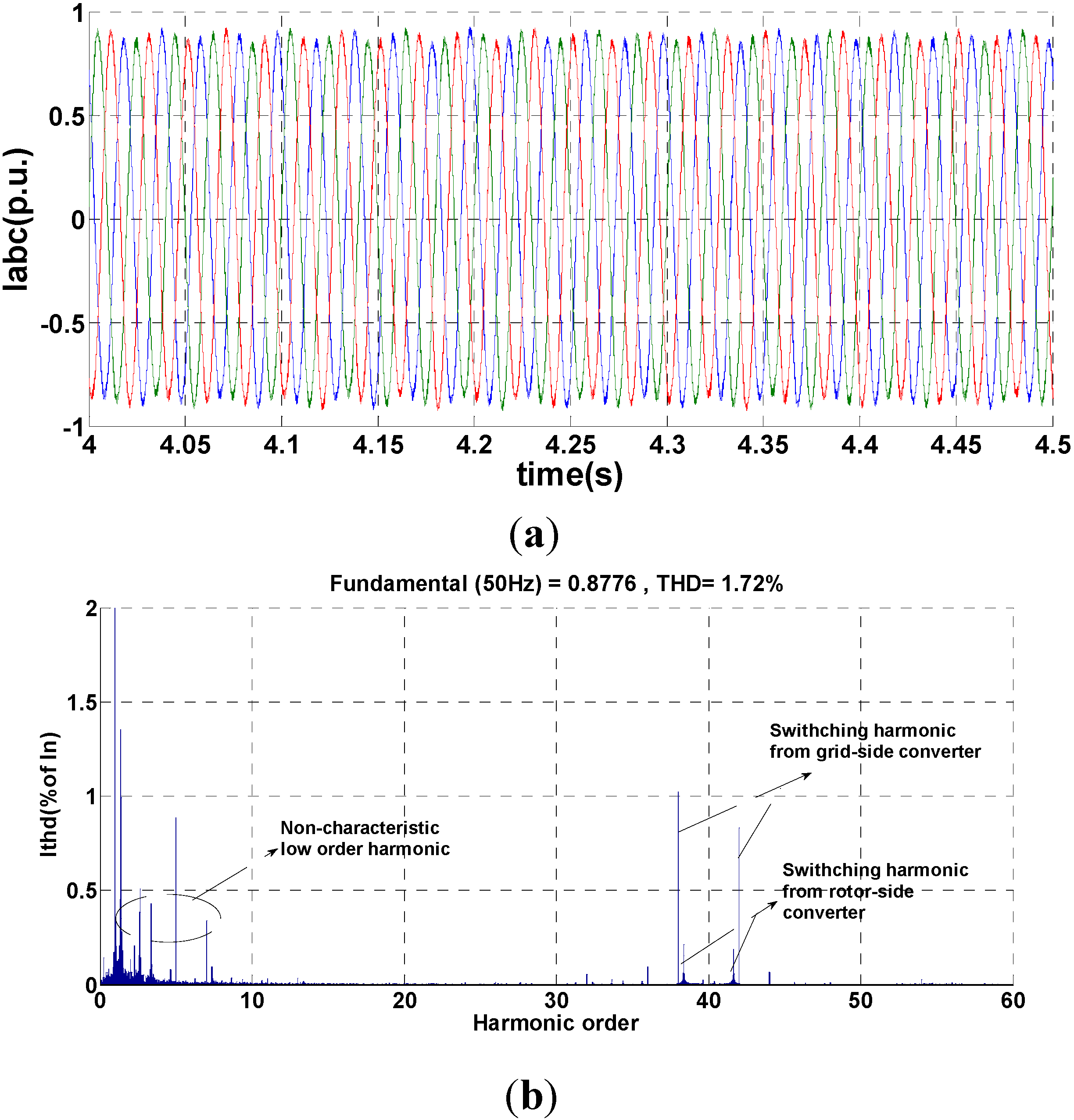
2.2.2. High Order Switching Harmonics

High order switching harmonics of DFIG with PWM controllers consist of two parts: the harmonic emission of the grid-side converter is directly injected into the grid system; the harmonic produced by the rotor-side converter intertwine through the electromagnetic coupling between the stator and rotor, and then is injected into the power grid through the stator.

The switching frequencies of the rotor-side and grid-side converters are set as f_rc and f_gc. And the harmonic voltage of the grid-side converter is calculated by Equation (10) [37]:

(10)

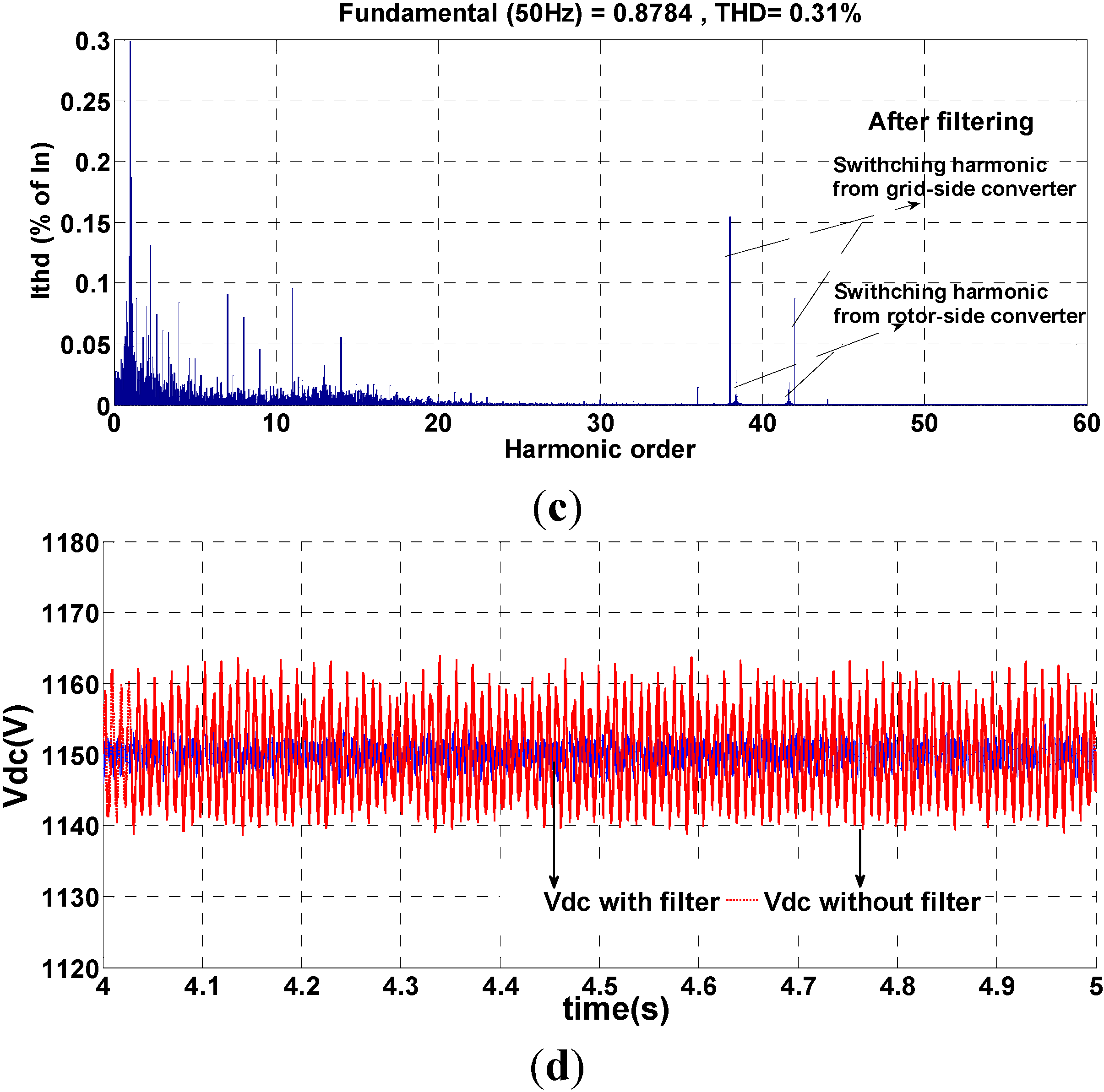
where M is the modulation index amplitude; and V_dc is the DC side voltage. Normally, V_dc is constant by the optimal control strategy of the grid-side converter. Then the amplitude of the output harmonic voltage is determined by M.

As the fundamental frequency of the grid-side converter is f_e = 50 Hz, the switching harmonic orders of the grid-side converter contain: f_gc ± 2f_e, f_gc ± 4f_e, 2f_gc ± f_e, 2f_gc ± 5f_e, 2f_gc ± 7f_e, 3f_gc ± 2f_e, 3f_gc ± 4f_e… [38,39]. When the switching frequency is quite high (thousands of Hz), f_gc ± 2f_e is the only harmonic order we need to consider. Other switching frequencies are ignored due to their small amplitude.

On the other hand, the control strategy of DFIG is constant frequency with variable speed. The reference frequency of the rotor-side converter is |sf_e|. Then the switching harmonic emissions of the rotor-side converter are injected into the grid through the air gap magnetic field between the stator and rotor.

Similar to the harmonic emissions of the grid-side converter, the switching harmonic order of the rotor-side converter is f_rc ± 2|sf_e|.

If f_rc ± 2|sf_e| = (6m + 1)|sf_e|,

f_s = f_r + f_m = f_rc ± 2|sf_e| + (1 − s)f_e, $slip=\frac{f_s-f_m}{f_s}=\frac{f_{rc}\pm 2\left|s{f}_e\right|}{f_{rc}\pm 2\left|s{f}_e\right|+(1-s)f_e}$;

If f_rc ± 2|sf_e| = (6m − 1)|sf_e|,

f_s = f_r − f_m = f_rc ± 2|sf_e| − (1 − s)f_e, $slip=\frac{f_s+f_m}{f_s}=\frac{f_{rc}\pm 2\left|s{f}_e\right|}{f_{rc}\pm 2\left|s{f}_e\right|-(1-s)f_e}$.

According to the steady state of DFIG in Figure 2, V_sh = 0 if there aren’t any background harmonics, the switching harmonic current emissions are affected by $V_r^{\prime }$, $\frac{{\omega }_s}{{\omega }_e}=\frac{f_{rc}\pm 2\left|s{f}_e\right|\pm (1-s)f_e}{f_e}$ and slip. But the switching harmonic current emissions of the grid-side converter are only related to the output harmonic voltage.

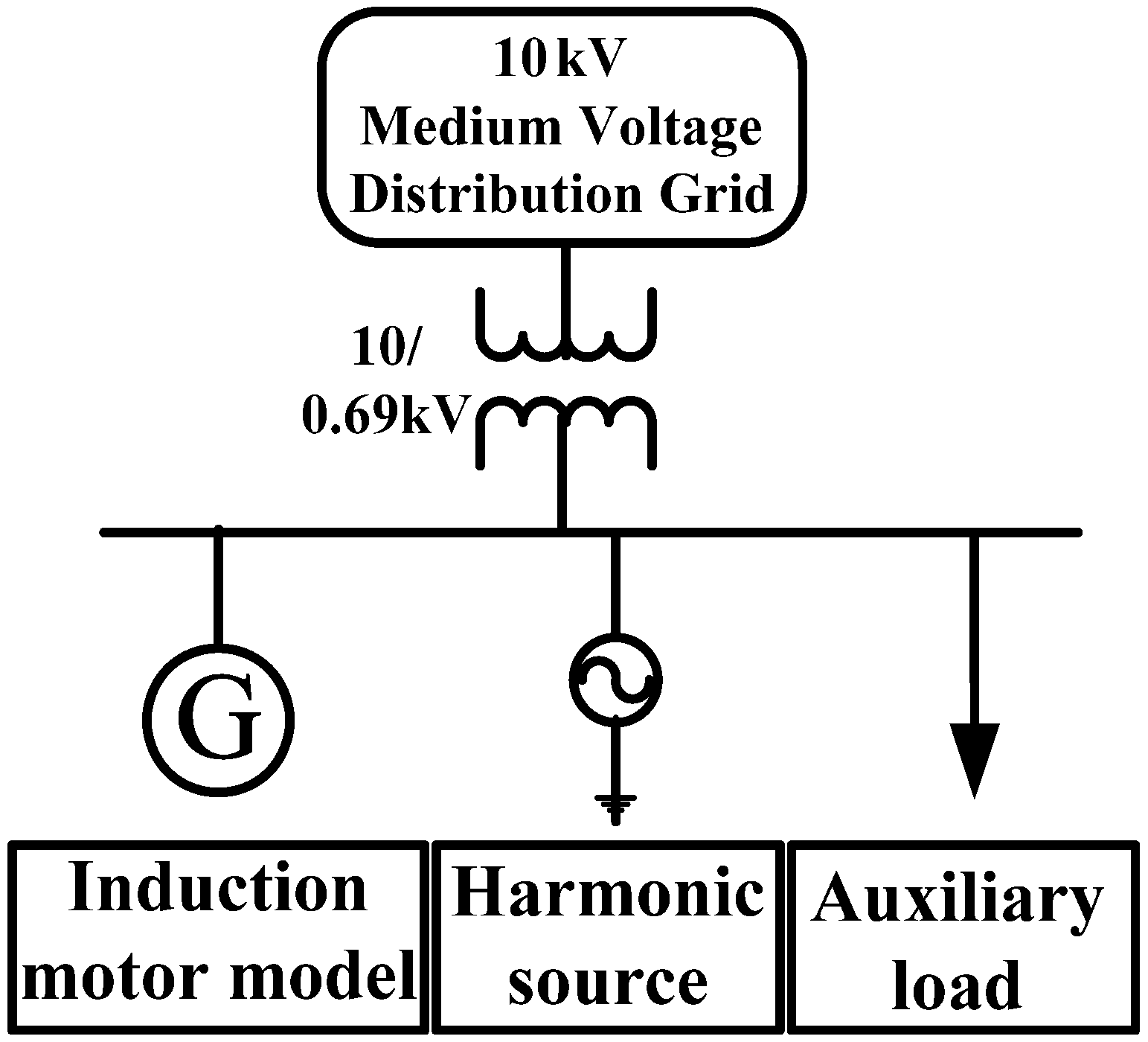
Non-characteristic and switching harmonic emissions of DFIG are discussed in this section. In order to study the harmonic propagation, the harmonic source model of DFIG is given in Figure 5. It consists of three parts: induction motor model is based on Figure 2; harmonic source part is the non-characteristic or switching harmonic emissions; auxiliary load is the supply load in the wind farm, and it can also be compensation devices.

Figure 5. The diagram of the harmonic source model of DFIG.

Figure 5. The diagram of the harmonic source model of DFIG.

3. Harmonic Source and Power Flow Modeling

3.1. Harmonic Admittance Matrix Model of Nonlinear Loads

In this paper, AC/DC converters installed in the distribution grid are the nonlinear harmonic sources. The harmonic coupled admittance matrix models are utilized to analyze the harmonic emissions of AC/DC converters [15]. The matrix models are adjusted to calculate the harmonic propagation and integration between the integrated wind farm and nonlinear loads.

The topological diagram of AC/DC converter with the equivalent load is shown in Figure 6. E_dc is the equivalent voltage source on the DC side; R_dc is the equivalent resistance; L is the DC side smoothing inductance, commutation angle and inductance are μ and L_C; α is the thyristor firing angle; I_dc is the DC current mean value; V_dc is the DC voltage mean value; V_ac is the DC side phase voltage.

Figure 6. The circuit diagram of AC/DC converter with the equivalent load.

Figure 6. The circuit diagram of AC/DC converter with the equivalent load.

Five converters are studied in this paper, the active and reactive power of each converter can be calculated by Equation (11):

(11)

where Uⁱ is the mean value of fundamental phase voltage at bus i, (i =1,..,5); L_ic and μ_i are the commutation inductance and angle of the number i converter; and α_i is the thyristor firing angle.

When the active and reactive powers of five converters are set as constant values, α_i and μ_i can be solved by Equation (11) based on the Newton-Raphson method. And the DC equivalent voltage source E_idc is given by Equation (12):

$$E_{idc}=\frac{3\sqrt{6}{U}^i}{2\pi }[\text{cos }{\alpha }_i+\text{cos}({\alpha }_i+{\mu }_i)]-\frac{\sqrt{6}{U}^i}{2\omega L_{idc}}[\text{cos }{\alpha }_i-\text{cos}({\alpha }_i+{\mu }_i)]R_{dc}$$

(12)

The harmonic admittance matrix of the converter is given by Equation (13), which establishes the frequency-domain linear relationship between harmonic voltage and current on the AC side [15]:

(13)

where ; the subscript i means the number i converter, the matrix parameters $Y_{Ah,k}^{+}$, $Y_{Ah,k}^{-}$ are given by Equations (14–16):

(14)

(15)

(16)

where A = 1, if h = 1,7,13,19,…; A = −1, if h = 5,11,17,23,…; B = 1, if h = 7,13,19,…; B = −1, if h = 5,11, 17,23,…; C = 1, if h = 1,7,13,19,…; C = −1, if h = 5,11,17,23,…; T₁ and T₂ are integers, T₁ = h/6, T₂ = h/6+1.

3.2. Harmonic Power Flow Modeling with Wind Farm and Nonlinear Load

Fundamental voltage phase angle and magnitude of power flow are the basis of the parameter evaluation of the admittance matrix of converters. According to Section 2, the wind generation is set as P − Q(V) node, and the converters are set as PQ nodes in the fundamental power flow. V_iAl∠φ_iAl is calculated from the fundamental power flow, and α_i, μ_i, E_idc are given by Equations (11) and (12). Then the harmonic coupled admittance matrix is built based on Equation (13). The other devices in the network are linear, and the node admittance matrix is shown in Equation (17):

(17)

The harmonic power flow results are given by Equation (18) which reflects the admittance matrix of the distribution network, nonlinear converters and wind farm:

(18)

where and I_{h_wind} reflect the harmonic characteristic of nonlinear converters and wind farm.

Define D = Y⁺ − Y_h = D_X + jD_Y, and then Equation (18) is transformed into Equation (19):

(19)

The result of Equation (19) is given by Equation (20):

(20)

where .

4. Harmonic Propagation and Interaction between Wind Farm and Nonlinear Loads in the Simulation Network

4.1. Introduction of the Simulation Network

In order to verify the proposed models and method, a medium voltage distribution network is built based on the network benchmarks of CIGRE Task Force C6.04.02 [40]. The network benchmarks have been used in some European projects [41]. In this paper, the average voltage is set as 10 kV, and five converters are connected to the medium voltage network by the 10/0.4 transformers, as shown in Figure 7. The simulation system is established in PSCAD/EMTDC. The linear load and line parameters of the simulation system are given in reference [41]. A small-scale wind farm is installed at bus 3 to study the harmonic propagation between wind turbines and nonlinear loads. The wind farm consists of 3 × 1.5 MW DFIG wind turbines connected to the medium voltage grid by the 10/0.69 kV transformers, and the parameter values of DFIG are given in Table 1.

Table 1. The parameters of DFIG.

Rs (p.u.)	Ls (p.u.)	$R_r^{\prime }$ (p.u.)	$L_r^{\prime }$ (p.u.)
0.016	0.125	0.011	0.111
Lm (p.u.)	Vdc (V)	fg (Hz)	frc (Hz)
2.013	1150	2000	2000

Table 1. The parameters of DFIG.

Rs (p.u.)	Ls (p.u.)	$R_r^{\prime }$ (p.u.)	$L_r^{\prime }$ (p.u.)
0.016	0.125	0.011	0.111
Lm (p.u.)	Vdc (V)	fg (Hz)	frc (Hz)
2.013	1150	2000	2000

Figure 7. The simulation network with the small-scale wind farm and nonlinear loads.

Figure 7. The simulation network with the small-scale wind farm and nonlinear loads.

4.2. Harmonic Evaluation of Nonlinear Loads in Different Conditions

The harmonic coupled admittance matrix model in Section 3 is used to evaluate the harmonic emissions of the AC/DC converters’ nonlinear load. When there is no wind farm installed in the distribution network, the nonlinear loads are set as PQ nodes in the fundamental power flow. The fundamental voltage value of each nonlinear load is 400 V, and the active and reactive power values of the five nonlinear loads at different buses are given in Table 2. According to Equations (11) and (12), the parameters of nonlinear loads are calculated, as shown in Table 3.

Table 2. The power values of five nonlinear loads.

Power	Bus12	Bus13	Bus14	Bus15	Bus16
P (kW)	147	58	105	163	67
Q (kW)	91	36	65	101	42

Table 2. The power values of five nonlinear loads.

Power	Bus12	Bus13	Bus14	Bus15	Bus16
P (kW)	147	58	105	163	67
Q (kW)	91	36	65	101	42

Table 3. The parameter values of nonlinear loads without wind farm.

Bus No.	Magnitude of voltage (p.u.)	Phase angle of voltage (°)	α (°)	μ (°)	Edc (V)
12	0.995	−124.454	31.473	0.614	405.039
13	0.991	−124.278	31.207	0.885	404.200
14	0.993	−124.387	31.140	1.172	405.696
15	0.990	−124.507	31.329	0.742	403.936
16	0.991	−124.291	31.384	0.748	403.671

Table 3. The parameter values of nonlinear loads without wind farm.

Bus No.	Magnitude of voltage (p.u.)	Phase angle of voltage (°)	α (°)	μ (°)	Edc (V)
12	0.995	−124.454	31.473	0.614	405.039
13	0.991	−124.278	31.207	0.885	404.200
14	0.993	−124.387	31.140	1.172	405.696
15	0.990	−124.507	31.329	0.742	403.936
16	0.991	−124.291	31.384	0.748	403.671

Based on the equivalence parameters of nonlinear loads, the harmonic coupled admittance matrix model is built by Equations (13–16). According to Equations (17–20), the harmonic emissions of nonlinear loads in the simulation network are calculated in MATLAB. In order to verify the harmonic coupled admittance matrix model, the harmonic emissions of the nonlinear loads are collected from the time-domain simulation in PSCAD/EMTDC. The comparison results are shown in Figure 8.

The V_thd values of each nonlinear load in MATLAB and PSCAD/EMTDC are almost the same, as shown in Figure 8, so the harmonic admittance matrix model established in MATALB can accurately evaluate the harmonic distortion of nonlinear power electronic loads.

Furthermore, when the small-scale wind farm is installed in the distribution grid, the fundamental power flow becomes fluctuant, and the equivalence parameters of nonlinear loads are not constant.

The capacity of the small-scale wind farm is P_{wind_total} = 3 × 1.5 MW = 4.5 MW, and P_{wind_total} is set as the fundamental value of wind farm. Ten initial wind power values are from 0 to 1 p.u. in intervals of 0.1 p.u. The fundamental voltage value of each nonlinear load is 400 V.

The small-scale wind farm is set as P – Q(V) node, and the expanding Newton-Raphson power flow method is applied in the fundamental power flow calculation. And then the parameter evaluations of converters at different buses are given by Equations (11–16). The final results of the fundamental voltage, parameter evaluation and harmonic emission at bus 12 are shown in Table 4.

Figure 8. The comparison of V_thd values of five nonlinear loads between harmonic coupled admittance matrix model and simulation results.

Figure 8. The comparison of V_thd values of five nonlinear loads between harmonic coupled admittance matrix model and simulation results.

Table 4. The parameters and harmonic distortion level of the nonlinear load at bus 12.

Pwind (p.u.)	Magnitude of voltage (p.u.)	Phase angle of voltage (°)	α (°)	μ (°)	Edc (V)	Vthd (%)
0	0.995	−124.454	31.473	0.614	405.039	4.2
0.1	1.001	−124.081	31.477	0.607	408.296	4.1
0.2	1.008	−123.708	31.481	0.599	411.506	4.1
0.3	1.014	−123.338	31.484	0.592	414.685	4.0
0.4	1.020	−122.966	31.490	0.584	417.837	4.0
0.5	1.026	−122.596	31.495	0.577	420.941	3.9
0.6	1.032	−122.226	31.500	0.571	424.019	3.9
0.7	1.038	−121.694	31.505	0.564	427.057	3.8
0.8	1.044	−121.487	31.510	0.558	430.072	3.8
0.9	1.050	−121.118	31.514	0.551	433.052	3.7
1	1.056	−120.751	31.519	0.545	435.997	3.7

Table 4. The parameters and harmonic distortion level of the nonlinear load at bus 12.

Pwind (p.u.)	Magnitude of voltage (p.u.)	Phase angle of voltage (°)	α (°)	μ (°)	Edc (V)	Vthd (%)
0	0.995	−124.454	31.473	0.614	405.039	4.2
0.1	1.001	−124.081	31.477	0.607	408.296	4.1
0.2	1.008	−123.708	31.481	0.599	411.506	4.1
0.3	1.014	−123.338	31.484	0.592	414.685	4.0
0.4	1.020	−122.966	31.490	0.584	417.837	4.0
0.5	1.026	−122.596	31.495	0.577	420.941	3.9
0.6	1.032	−122.226	31.500	0.571	424.019	3.9
0.7	1.038	−121.694	31.505	0.564	427.057	3.8
0.8	1.044	−121.487	31.510	0.558	430.072	3.8
0.9	1.050	−121.118	31.514	0.551	433.052	3.7
1	1.056	−120.751	31.519	0.545	435.997	3.7

From Table 4, it is found that the parameters of the nonlinear load vary with different wind power values. The differences among the thyristor firing angle α values are quite small, and the phase angle of voltage and commutation angle μ change a little. The fluctuant wind power induces the variable fundamental voltage, and then the harmonic emissions of nonlinear loads change, as shown in Table 4. And the V_thd value of the nonlinear load at bus 12 changes from 4.2% to 3.7%.

4.3. Harmonic Source Modeling of the Small-Scale Wind Farm

4.3.1. High Order Switching Harmonic Analysis

In order to analysis the switching high order harmonic emissions, a detailed model of the small-scale wind farm is built in MATLAB/SIMULINK. PWM control strategies of the rotor and grid side converters are based on reference [22]. The parameter values of DFIGs are given in Table 1.

Due to the sinusoidal distributions of the stator and rotor windings in the detailed model, the switching harmonics are the main components. When the output power of the small-scale wind farm is 4.5 MW, the current emission without filter is shown in Figure 9a.

From Figure 9b,c, the switching harmonic emissions of the grid-side converter are higher than the rotor-side converter. The harmonic orders of the grid-side converter are 42 Hz and 38 Hz. The harmonic orders of the rotor-side converter are 40 ± 1.63 Hz. These harmonic orders conform to the deduction in Section 2.2. Comparing the Figure 9b,c, it is found that the low pass filter reduces the high order switching harmonic effectively. In Figure 9d, the ripple of the DC voltage is apparently repressed by the filter, and then the low order harmonics are reduced.

Figure 9. Switching harmonic simulation. (a) Currents of the small-scale wind farm without filter; (b) I_thd without filter; (c) I_thd with filter; (d) Comparison of V_dc with and without filter.

Figure 9. Switching harmonic simulation. (a) Currents of the small-scale wind farm without filter; (b) I_thd without filter; (c) I_thd with filter; (d) Comparison of V_dc with and without filter.

After using the filter, the high order switching harmonic currents are small enough to merge into the grid. Because wind power varies with the random wind speed, the rotor speed and slip are both variable. In Table 5, five different wind speeds are calculated in the model and the relationship between the switching harmonics and slips are studied. It is found that the slip s changes from −0.21 to 1.8 and the switching harmonic orders of the rotor-side converter are changed. Because the switching harmonic currents from the rotor-side converter are too small, only the switching harmonic currents of the grid-side converter are of interest in this paper.

Table 5. The comparison of two kinds of switching harmonics with different slips.

Vw (m/s)	P (MW)	S	I1 (A)	Ir-sh order	|Ir-sh| (A)	Ih_grid order	|Ih_grid| (A)
5	0.23	0.18	192.45	40 + 0.46	0.71	40 + 2	3.08
				40 − 0.46	0.75	40 − 2	5.39
7	0.86	0.12	715.41	40 + 0.64	0.36	40 + 2	3.15
				40 − 0.64	0.43	40 − 2	5.51
9	1.80	−0.02	1506.13	40 + 1.02	0	40 + 2	3.19
				40 − 1.02	0	40 − 2	5.57
11	3.22	−0.17	2692.63	40 + 1.5	0.58	40 + 2	3.28
				40 − 1.5	0.87	40 − 2	5.79
13	4.5	−0.21	3765.33	40 + 1.63	0.68	40 + 2	3.29
				40 − 1.63	1.054	40 − 2	5.81

Table 5. The comparison of two kinds of switching harmonics with different slips.

Vw (m/s)	P (MW)	S	I1 (A)	Ir-sh order	|Ir-sh| (A)	Ih_grid order	|Ih_grid| (A)
5	0.23	0.18	192.45	40 + 0.46	0.71	40 + 2	3.08
				40 − 0.46	0.75	40 − 2	5.39
7	0.86	0.12	715.41	40 + 0.64	0.36	40 + 2	3.15
				40 − 0.64	0.43	40 − 2	5.51
9	1.80	−0.02	1506.13	40 + 1.02	0	40 + 2	3.19
				40 − 1.02	0	40 − 2	5.57
11	3.22	−0.17	2692.63	40 + 1.5	0.58	40 + 2	3.28
				40 − 1.5	0.87	40 − 2	5.79
13	4.5	−0.21	3765.33	40 + 1.63	0.68	40 + 2	3.29
				40 − 1.63	1.054	40 − 2	5.81

In practice, a wind generator may not comprise a neutral conductor or a ground return path, and the transformer windings are delta connected, so the wind farm will not inject zero-sequence harmonic currents into the grid [42]. The 42th switching harmonic currents can’t be injected into the grid, so only the 38th switching harmonic currents are analyzed. From Table 5, the 38th switching harmonic current changes from 5.39 to 5.81 A, the difference is small. At the same time, the harmonic emissions of nonlinear loads are low orders, and there is little interaction between the 38th switching harmonic current and nonlinear loads, so the 38th harmonic voltage at bus 3 is directly calculated by the harmonic admittance matrix, V_38thd = 0.7%. Though the amplitude of the high order switching harmonic is not high, it may induce large fluctuant when the resonance occurs at higher frequency.

4.3.2. Non-Characteristic Low Order Harmonic Analysis

Due to the random wind speed and variable environment, the real output power data of the small-scale wind farm are fluctuant and non-stationary. In Figure 10, the active power data of the small-scale wind farm in a month is collected with a ten minute sampling interval.

The scatter plots of the fifth and seventh harmonic current X-Y projections are shown in Figure 11. The reference value is the percentage of rated current I_N, and I_N = 245 A. Accord to the scatter plots, the pdfs of the X and Y components of the seventh harmonic currents can be fitted with Gaussian distribution and the parameters are r_X7Y7 = 0.18, μ_X7 = −0.025, μ_Y7 = −0.085, σ_X7 = 0.35, σ_Y7 = 0.29.

Figure 10. Wind power data in 31 days with 10 min intervals.

Figure 10. Wind power data in 31 days with 10 min intervals.

Figure 11. Scatter plots of wind farm harmonic current X-Y projections. (a) The fifth harmonic currents; (b) The seventh harmonic currents.

Figure 11. Scatter plots of wind farm harmonic current X-Y projections. (a) The fifth harmonic currents; (b) The seventh harmonic currents.

Different from the seventh harmonic currents, the pdfs of X and Y components of the fifth harmonic current can’t be approximated by Gaussian distribution, as shown in Figure 11a. And the correlation coefficient of the fifth harmonic current is r_XsYs = −0.746. The pdf of X components of the fifth harmonic current is verified by the Normal probability plot which can graphically assess whether the data could be fitted with Normal distribution. The pdf is not fitted with a Normal distribution because the plot in Figure 12b is not linear.

Figure 12. Pdfs of the fifth harmonic current and Normal verification. (a) Pdfs of X and Y components; (b) The Normal probability verification plot.

Figure 12. Pdfs of the fifth harmonic current and Normal verification. (a) Pdfs of X and Y components; (b) The Normal probability verification plot.

Due to the complicated distribution of the fifth harmonic currents, the common distributions like Weibull, Rayleigh and Gaussian distributions are unsuitable, so GGMM are proposed to analyze the fifth harmonic propagation of wind generators.

(i) GMM of X and Y components

The parameters of GMM are estimated by EM method, and the observed data are the fifth harmonic current emissions of wind generators, as shown in Figure 11a. The GMM order is set as M = 2, and the divided results of the fifth harmonic current are given in Table 6.

Table 6. The divided results of the fifth harmonic current.

Reference axis	Coefficient	Mean value (μ)	Standard deviation (σ)
X	εx1 = 0.774	μx1 = −0.098	σx1 = 0.117
	εx2 = 0.226	μx2 = −0.944	σx2 = 0.576
Y	εy1 = 0.794	μy1 = −0.268	σy1 = 0.129
	εy2 = 0.206	μy2 = 0.339	σy2 = 0.467

Table 6. The divided results of the fifth harmonic current.

Reference axis	Coefficient	Mean value (μ)	Standard deviation (σ)
X	εx1 = 0.774	μx1 = −0.098	σx1 = 0.117
	εx2 = 0.226	μx2 = −0.944	σx2 = 0.576
Y	εy1 = 0.794	μy1 = −0.268	σy1 = 0.129
	εy2 = 0.206	μy2 = 0.339	σy2 = 0.467

(ii) Clustering the Gaussian components of the fifth harmonic currents

Due to the fact that r_XsYs = −0.746, I_x5 and I_y5 are statistically dependent. Four central phasors are defined as μ_xm + jμ_yn, (m, n = 1, 2). The fifth harmonic current phasors are divided into four clusters according to the optimal phasor clustering method, and the division axis are X = −0.4 and Y = 0.041, as shown in Table 7.

Table 7. The clustering results of the optimal phasor clustering method.

Coefficient	Mean value	Standard deviation	Mean value	Standard deviation
εx = 0.788	μx1 = −0.098	σx1 = 0.117	μy1 = −0.273	σy1 = 0.131
ε2 = 0.148	μx2 = −1.164	σx2 = 0.518	μy2 = 0.552	σy2 = 0.333
ε3 = 0.051	μx1 = −0.755	σx1 = 0.374	μy2 = −0.233	σy2 = 0.174
ε4 = 0.011	μx2 = −0.182	σx2 = 0.129	μy1 = 0.223	σy1 = 0.241

Table 7. The clustering results of the optimal phasor clustering method.

Coefficient	Mean value	Standard deviation	Mean value	Standard deviation
εx = 0.788	μx1 = −0.098	σx1 = 0.117	μy1 = −0.273	σy1 = 0.131
ε2 = 0.148	μx2 = −1.164	σx2 = 0.518	μy2 = 0.552	σy2 = 0.333
ε3 = 0.051	μx1 = −0.755	σx1 = 0.374	μy2 = −0.233	σy2 = 0.174
ε4 = 0.011	μx2 = −0.182	σx2 = 0.129	μy1 = 0.223	σy1 = 0.241

It can be found that the first and second part are the main components, and their correlation coefficients are r₁ = 0.07 and r₂ = −0.44.

(iii) Generalized Gamma distribution

Based on GMM and phasor clustering, the observed data of the fifth harmonic currents are clustered into four Gaussian components. Each component can be approximated by GGD, so GGMM of the fifth harmonic current emissions are given by Equation (21):

(21)

The parameters in Equation (21) are from Table 7, and the first two parts can accurately approximate the pdfs due to their bigger weighted coefficients. Then the cdf of the fifth harmonic current is approximated by Rayleigh, Weibull, Normal distributions and GGMM, as shown in Figure 13.

The 95% value of the fifth harmonic voltages is defined as an index, CP₉₅, which is used to compare the different distributions. In Figure 13, CP₉₅ of GGMM and the actual data distribution are both 1.5 p.u., but CP₉₅ of Normal distribution, Weibull and Rayleigh distributions are 1.1 and 1.2 p.u., so the cdf of the fifth harmonic current can be more accurately approximated by the GGMM.

Figure 13. Cdf of the fifth harmonic current approximated by different distributions.

Figure 13. Cdf of the fifth harmonic current approximated by different distributions.

4.4. Harmonic Interaction between the Wind Farm and Nonlinear Loads

When a small-scale wind farm is installed in the distribution grid, the fundamental power flow changes with the fluctuating wind power, and then the equivalence parameters of nonlinear loads become variable, as shown in Table 4. At the same time, stochastic harmonic emissions are calculated in the harmonic power flow analysis based on Equations (11–14). Because the influence of the wind farm operating point on harmonic current is small, the power level and harmonic emissions of the wind farm are analyzed independently.

First, the fluctuating wind power values are divided into ten intervals which are from 0 to 1 p.u. with intervals of 0.1 p.u. In Table 4, the changes of the parameter values and V_thd of the nonlinear load in each interval are quite small, so the parameters of nonlinear loads are set as fixed values in each interval. Then the probability value of random wind power in each interval is set as the weighted coefficient. Based on the real wind power data in Figure 10, the weighted coefficient in each interval is calculated and shown in Table 8.

Table 8. The weighted coefficient in each interval.

Interval	(0, 0.1) p.u.	(0.1, 0.2) p.u.	(0.2, 0.3) p.u.	(0.3, 0.4.) p.u	(0.4, 0.5) p.u.
weighted coefficient	0.416	0.147	0.114	0.087	0.056
Interval	(0.5, 0.6.) p.u	(0.6, 0.7) p.u.	(0.7, 0.8) p.u.	(0.8, 0.9) p.u.	(0.9, 1.0) p.u.
weighted coefficient	0.049	0.029	0.032	0.027	0.042

Table 8. The weighted coefficient in each interval.

Interval	(0, 0.1) p.u.	(0.1, 0.2) p.u.	(0.2, 0.3) p.u.	(0.3, 0.4.) p.u	(0.4, 0.5) p.u.
weighted coefficient	0.416	0.147	0.114	0.087	0.056
Interval	(0.5, 0.6.) p.u	(0.6, 0.7) p.u.	(0.7, 0.8) p.u.	(0.8, 0.9) p.u.	(0.9, 1.0) p.u.
weighted coefficient	0.049	0.029	0.032	0.027	0.042

In Table 8, the bigger weighted coefficients are in the smaller wind power interval. And the parameter values of nonlinear loads in each interval are from Table 4. For example, α in (0, 0.1 p.u.) is the average value while P_wind = 0 and P_wind = 0.1 p.u..

Due to the independent relationship between wind harmonic emission and power level, the same pdf of wind harmonic emission is utilized in each interval. According to the results in Section 4.3, the pdfs of the fifth and seventh harmonic current of wind power are both accurately approximated by GGMM.

Then the harmonic interaction between the wind farm and nonlinear loads are analyzed by Equations (17–20). I_s in Equation (20) reflects the harmonic characteristic of nonlinear load, and I_{h_wind} represents the wind harmonic current emissions. And Equation (20) is changed into Equation (22):

(22)

where represents the harmonic propagation of nonlinear loads, represents the wind harmonic propagation.

In each interval the parameters of the harmonic admittance matrix are fixed, and the probability function of ${\dot{V}}_{h\_wind}$ is the linear combination of I_{h_wind} which consists of the fifth and seventh harmonic emissions.

Based on the above complete formula derivation, statistical characteristic of each bus voltage is analyzed and reflected by the generalized gamma mixture models. For example, the statistical results of the nonlinear load at bus 3 in the first interval (0, 0.1 p.u.), in which s = 0.2, are given in the Table 9.

Table 9. Statistical characteristic of harmonic voltage at bus 3.

Harmonic order	Coefficient (εm)	Rectangular components	Mean value (μ)	Standard deviation (σ)	Correlation coefficient (r)
5	ε1 = 0.8	VX	−0.9212	0.0405	−0.1084
		VY	−0.2454	0.0391
	ε2 = 0.2	VX	−1.1793	0.1327	0.5812
		VY	−0.4918	0.1479
7	ε1 = 0.8	VX	0.4343	0.0363	0.2992
		VY	0.6935	0.04662
	ε2 = 0.2	VX	0.4354	0.0363	0.2998
		VY	0.6956	0.04666
11	ε1 = 0.8	VX	0.6340	0.0006	−1
		VY	−0.2703	0.0002
	ε2 = 0.2	VX	0.6340	0.0014	−1
		VY	−0.2706	0.0006

Table 9. Statistical characteristic of harmonic voltage at bus 3.

Harmonic order	Coefficient (εm)	Rectangular components	Mean value (μ)	Standard deviation (σ)	Correlation coefficient (r)
5	ε1 = 0.8	VX	−0.9212	0.0405	−0.1084
		VY	−0.2454	0.0391
	ε2 = 0.2	VX	−1.1793	0.1327	0.5812
		VY	−0.4918	0.1479
7	ε1 = 0.8	VX	0.4343	0.0363	0.2992
		VY	0.6935	0.04662
	ε2 = 0.2	VX	0.4354	0.0363	0.2998
		VY	0.6956	0.04666
11	ε1 = 0.8	VX	0.6340	0.0006	−1
		VY	−0.2703	0.0002
	ε2 = 0.2	VX	0.6340	0.0014	−1
		VY	−0.2706	0.0006

According to Table 9, the probability distribution of the fifth harmonic voltage at bus 3 in (0, 0.1 p.u.) is combined by two GGD parts of which the coefficients are ε₁ = 0.8 and ε₂ = 0.2. This is mainly caused by the GGMM of the fifth harmonic current emissions of the wind farm. Different from the fifth harmonic voltage, the characteristics of the seventh harmonic voltage with two coefficients are almost the same. This means that the mixture pdfs of the fifth harmonic current emissions of wind farm mainly affect the fifth harmonic voltage. Furthermore, the standard deviation of the eleventh harmonic voltage is very close to zero which means that the eleventh harmonic voltage is almost constant.

So the fifth and seventh harmonic voltages at bus 3 are analyzed by probability distribution models. The higher order harmonic voltages at bus 3 are nearly constant and directly solved. There are ten intervals for the harmonic propagation and interaction evaluation, and all of them are calculated. The probability characteristics of the fifth and seventh harmonic voltage in (0, 0.1 p.u) and (0.9 p.u., 1.0 p.u.) are compared, in Figure 14.

Figure 14. Pdfs of the harmonic voltages at bus 3 in different intervals. (a) The fifth harmonic voltage magnitude; (b) The seventh harmonic voltage magnitude.

Figure 14. Pdfs of the harmonic voltages at bus 3 in different intervals. (a) The fifth harmonic voltage magnitude; (b) The seventh harmonic voltage magnitude.

The pdf of the fifth harmonic voltage at bus 3 is approximated by GGMM, and the pdfs in (0, 0.1 p.u) and (0.9 p.u., 1 p.u.) are shown in Figure 14a (real line) and Figure 14a (dashed line). Then the pdf of the seventh harmonic voltage at bus 3 is shown in Figure 14b. The harmonic voltage distribution in the higher interval is closer to zero because the wind power in the higher interval is larger. Larger wind power improves the fundamental voltage, and then the voltage harmonic distortion level is reduced.

The index CP₉₅ is used to evaluate the cdfs of the harmonic voltages at bus 3, and the cdfs of harmonic voltages are shown in Figure 15. CP₉₅ of the fifth harmonic voltage in (0, 0.1 p.u) and (0.9 p.u., 1.0 p.u.) are 1.32% and 1.35%. The difference of CP₉₅ between the two intervals is quite small. Based on the Figure 14a, the main part of the pdf of the fifth harmonic voltage is closer to zero when the interval value is bigger. But the other part between 1.1% and 1.5% changes a little. The different CP₉₅ values reflect the final harmonic distortion level, and each part of the generalized gamma mixture models is important.

Different from the fifth harmonic voltage, V_X and V_Y of the seventh harmonic voltage at bus 3 are approximated by one Gaussian distribution. And the pdf of the seventh harmonic voltage is fitted with GGD which is the simplified type of GGMM. CP₉₅ of the seventh harmonic voltage in (0, 0.1 p.u) and (0.9 p.u., 1.0 p.u.) are 0.88% and 0.94%, as shown in Figure 15b.

Similar to the harmonic analysis in (0, 0.1 p.u) and (0.9 p.u., 1.0 p.u.), pdfs and cdfs of harmonic voltage at different buses are analyzed. Then the final pdf and cdf of the harmonic voltage are the linear combination of ten intervals with different weighted coefficients. The comparison of the cdfs of the harmonic voltages at bus 3 between GGMM and simulation results in PSCAD/EMTDC is shown in Figure 16.

Figure 15. Cdfs of the harmonic voltages at bus 3 in different intervals. (a) The fifth harmonic voltage magnitude; (b) The seventh harmonic voltage magnitude.

Figure 15. Cdfs of the harmonic voltages at bus 3 in different intervals. (a) The fifth harmonic voltage magnitude; (b) The seventh harmonic voltage magnitude.

Figure 16. Cdfs of the harmonic voltages at bus 3 approximated by GGMM, Gaussian distribution and simulation results. (a) The fifth harmonic; (b) The seventh harmonic.

Figure 16. Cdfs of the harmonic voltages at bus 3 approximated by GGMM, Gaussian distribution and simulation results. (a) The fifth harmonic; (b) The seventh harmonic.

In Figure 16a, CP₉₅ of the fifth harmonic voltage based on the simulation results is 1.29%, and CP₉₅ based on the proposed GGMM combined with the harmonic admittance matrix model is 1.33%. The difference between the proposed model and simulation result is quite small. Then CP₉₅ of the seventh harmonic voltage based on the proposed models and simulation results are 0.93% and 0.94%. If the pdf of the fifth harmonic current is directly approximated by Gaussian distribution, the CP₉₅ values of the fifth and seventh harmonic voltage are 1.18% and 0.88%. The error is quite big, and it can’t guarantee the high power quality level. Compared with the Gaussian distribution, the GGMM combined with the harmonic admittance matrix model simulate and evaluate the propagation and interaction between the small-scale wind farm and nonlinear loads more accurately.

5. Conclusions

The integration of a small-scale wind farm in the distribution grid brings about some challenges to the system safety and reliability. Non-stationary wind power induces a fluctuating fundamental power flow, and the non-characteristic harmonic currents of the wind farm interact with the harmonic emissions of nonlinear loads. In this paper, the fundamental power flow is calculated by the expanding Newton-Raphson method due to the P – Q(V) characteristic of wind turbines. Generalized gamma mixture models are proposed to approximate the pdf of harmonic emissions, which are more effective than general distributions such as the Gaussian, Rayleigh and Weibull ones. Then the voltage harmonic distortion level of nonlinear loads combined with the wind farm is accurately evaluated by the harmonic admittance matrix model. The harmonic interaction between the wind farm and nonlinear loads are calculated by the proposed models. The final results in MATLAB and PSCAD/EMTDC reveal that the generalized gamma mixture and harmonic admittance matrix models accurately evaluate the harmonic propagation and interaction between the small-scale wind farm and nonlinear loads in the distribution grid.

References

1. Poul, S.; Nicolaos, A.C. Power fluctuations from large wind farms. IEEE Trans. Power Syst. 2007, 22, 958–965. [Google Scholar] [CrossRef]
2. Vittal, E.; Keane, A.; O’Malley, M. Varying Penetration Ratios of Wind Turbine Technologies for Voltage and Frequency Stability. In Proceeding of the 2008 IEEE Power and Energy Society General Meeting—Conversion and Delivery of Electrical Energy in the 21st Century, Pittsburgh, PA, USA, 20–24 July 2008; pp. 1–6.
3. Xie, G.L.; Zhang, B.H. Probabilistic harmonic analysis of wind generators based on generalized gamma mixture models. Mod. Phys. Lett. B 2013, 27, 1–12. [Google Scholar]
4. Kasem, A.H.; EI-Saadany, E.F.; EI-Tamaly, H.H. Ramp Rate Control and Voltage Regulation for Grid Directly Connected Wind Turbines. In Proceedings of the 2008 IEEE Power and Energy Society General Meeting—Conversion and Delivery of Electrical Energy in the 21st Century, Pittsburgh, PA, USA, 20–24 July 2008; pp. 31–36.
5. Wu, Y.C.; Ding, M. Simulation study on voltage fluctuations and flicker caused by wind farms. Power Syst. Technol. 2009, 33, 125–130. [Google Scholar]
6. Huang, N.E.; Shen, Z.; Steven, R.L. The empirical mode decomposition and the Hilbert spectrum for nonlinear and non-stationary time series analysis. Proc. R. Soc. 1998, 454, 903–995. [Google Scholar] [CrossRef]
7. Xu, Y.L.; Asce, M.; Chen, J. Characterizing non-stationary wind speed using empirical mode decomposition. J. Struct. Eng. 2004, 130, 912–920. [Google Scholar] [CrossRef]
8. Moreno, C.V.; Duarte, H.A.; Garcia, J.U. Propagation of flicker in electric power networks due to wind energy conversions systems. IEEE Trans. Energy Convers. 2002, 17, 267–272. [Google Scholar] [CrossRef]
9. Bradt, M.; Badrzadeh, B.; Camm, E. Harmonics and Resonance Issues in Wind Power Plants. In Proceedings of the 2011 IEEE Power and Energy Society General Meeting, San Diego, CA, USA, 24–29 July 2011; pp. 1–8.
10. Novanda, H.; Regulski, P.; Stanojevic, V. Assessment of frequency and harmonic distortions during wind farm rejection test. IEEE Trans. Sustain. Energy 2013, 4, 698–705. [Google Scholar] [CrossRef]
11. Larose, C.; Gagnon, R.; Homme, P.P. Type-III wind power plant harmonic emissions field measurements and aggregation guidelines for adequate representation of harmonics. IEEE Trans. Sustain. Energy 2013, 4, 797–804. [Google Scholar] [CrossRef]
12. Papathanassiou, S.A.; Papadopoulos, M.P. Harmonic analysis in a power system with wind generation. IEEE Trans. Power Deliv. 2006, 21, 2006–2016. [Google Scholar] [CrossRef]
13. Tentzerakis, S.T.; Papathanassiou, S.A. An investigation of the harmonic emissions of wind turbines. IEEE Trans. Energy Convers. 2007, 22, 150–158. [Google Scholar] [CrossRef]
14. Bonner, A.; Grebe, T.; Hopkins, L. Modeling and simulation of the propagation of harmonics in electric power networks. Part I: Concepts, models and simulation techniques. IEEE Trans. Power Deliv. 1996, 11, 452–465. [Google Scholar] [CrossRef]
15. Sun, Y.Y.; Zhang, G.B.; Xu, W. A harmonically coupled admittance matrix model for AC/DC converters. IEEE Trans. Power Syst. 2007, 22, 1574–1582. [Google Scholar] [CrossRef]
16. Liang, X.D.; Luy, Y.; Don, O.K. Investigation of Input Harmonic Distortions of Variable Frequency Drives. In Proceedings of the Industrial & Commercial Power Systems Technical Conference (ICPS 2007), Edmonton, Canada, 6–11 May 2007; pp. 1–11.
17. Verma, V.; Singh, B.; Chandra, A. Power conditioner for variable-frequency drives in offshore oil fields. IEEE Trans. Ind. Appl. 2010, 46, 731–739. [Google Scholar] [CrossRef]
18. Sharma, V.; Fleming, R.J.; Niekamp, L. An iterative approach for analysis of harmonic penetration in the power transmission networks. IEEE Trans. Power Deliv. 1991, 6, 1698–1706. [Google Scholar] [CrossRef]
19. Hu, W.H.; Wang, W.; Wang, Y.L.; Xiao, H.B. Power flow analysis in electrical power system including wind farms. North China Electr. Power 2006, 10, 12–15. [Google Scholar]
20. Li, Y.; Luo, Y.L.; Zhang, B.H.; Mao, C.X. A Modified Newton-Raphson Power Flow Method Considering Wind Power. In Proceedings of the 2011 Asia-Pacific Power and Energy Engineering Conference (APPEEC), Wuhan, China, 25–28 March 2011; pp. 1–5.
21. Feijoo, A.E.; Cidras, J. Modeling of wind farms in the load flow analysis. IEEE Trans. Power Syst. 2000, 15, 110–115. [Google Scholar] [CrossRef]
22. Miller, N.W.; Sanchez-Gasca, J.J.; Price, W.W. Dynamic Modeling of GE 1.5 and 3.6 MW Wind Turbine-Generators for Stability Simulations. In Proceedings of the IEEE Power Engineering Society General Meeting, Toronto, Canada, 13–17 July 2003; Volume 3, pp. 1977–1983.
23. Lindholm, M.; Ramussen, T.W. Harmonic Analysis of Doubly Fed Induction Generators. In Proceedings of the Fifth International Conference on Power Electronics and Drive Systems (PEDS 2003), Singapore, 17–20 November 2003; Volume 2, pp. 837–841.
24. Zhong, W.; Sun, Y.Z.; Li, G.J.; Li, Z.G. Stator current harmonics analysis of doubly-fed induction generator. Electr. Power Autom. Equip. 2010, 30, 1–5. [Google Scholar]
25. Fan, L.L.; Yuvarajan, S.; Kavasseri, R. Harmonic analysis of a DFIG for a wind energy conversion system. IEEE Trans. Energy Convers. 2010, 25, 181–189. [Google Scholar] [CrossRef]
26. King, R.; Ekanayake, J.B. Harmonic Modelling of Offshore Wind Farms. In Proceedings of the 2010 IEEE Power and Energy Society General Meeting, Minneapolis, MN, USA, 25–29 July 2010; pp. 1–6.
27. Schostan, S.; Dettmann, K.D.; Thanh, T.D.; Schulz, D. Harmonic Propagation in a Doubly Fed Induction Generator of a Wind Energy Converter. In Proceedings of the Compatibility and Power Electronics (CPE 2009), Badajoz, Spain, 20–22 May 2009; pp. 101–108.
28. Kiani, M.; Lee, W.J. Effects of voltage unbalance and system harmonics on the performance of doubly fed induction wind generators. IEEE Trans. Ind. Appl. 2010, 46, 562–568. [Google Scholar] [CrossRef]
29. Francesco, C.D.; Matteo, F.I.; Roberto, P. An observer for sensorless DFIM drives based on the natural fifth harmonic of the line voltage, without stator current measurement. IEEE Trans. Ind. Electr. 2013, 60, 4301–4309. [Google Scholar] [CrossRef]
30. Liu, C.J.; Blaabjerg, F.; Chen, W.J. Stator current harmonic control with resonant controller for doubly fed induction generator. IEEE Trans. Power Electr. 2012, 27, 3207–3220. [Google Scholar] [CrossRef]
31. Sainz, L.; Mesas, J.J.; Teodorescu, R. Deterministic and stochastic study of wind farm harmonic currents. IEEE Trans. Energy Convers. 2010, 25, 1071–1081. [Google Scholar] [CrossRef] [Green Version]
32. Cavallini, A.; Langella, R.; Testa, A. Gaussian Modeling of Harmonic Vectors in Power Systems. In Proceedings of the 8th International Conference on Harmonics and Quality of Power, Athens, Greece, 14–16 October 1998; pp. 1010–1017.
33. Baghzouz, Y.; Burch, R.F.; Capasso, A. Time-varying harmonics: II-harmonic summation and propagation. IEEE Trans. Power Syst. 2002, 17, 279–285. [Google Scholar] [CrossRef]
34. Wilson, R. Multiresolution Gaussian Mixture Models: Theory and Application; Research Report RR404; Department of Computer Science, University of Warwick: Warwickshire, UK, 1999. [Google Scholar]
35. Zhao, Y.X.; Zhuang, X.H.; Ting, J.S. Gaussian mixture density modeling of non-gaussian source for autoregressive process. IEEE Trans. Signal. Proc. 1995, 43, 894–903. [Google Scholar] [CrossRef]
36. Moon, T. The expectation-maximization algorithm. IEEE Signal. Proc. Mag. 1996, 13, 47–60. [Google Scholar] [CrossRef]
37. Lu, X.; Rogers, C.; Peng, F.Z. A Double Fourier Analysis Development of THD for PWM Inverters: A Theoretical Method for Motor Loss Minimization. In Proceedings of the 2010 IEEE Energy Conversion Congress and Exposition (ECCE), Atlanta, GA, USA, 12–16 September 2010; pp. 1505–1510.
38. Fioretto, M.; Raimondo, G.; Rubino, L. Evaluation of Current Harmonic Distortion in Wind Farm Application Based on Synchronous Active Front End Converters. In Proceedings of the IEEE African Conference (AFRICON 2011), Livingstone, Zambia, 13–15 September 2011; pp. 1–6.
39. Holmes, D.G.; Lipo, T.A. Pulse Width Modulation for Power Converters: Principles and Practice; IEEE Press Series on Power Engineering; John Wiley & Sons: Manhattan, NY, USA, 2003; pp. 140–144. [Google Scholar]
40. Papathanassiou, S.; Hatziargyriou, N.; Strunz, K. A Benchmark Low Voltage Microgrid Network. In Proceedings of the International Conference on Large High Voltage Electric System (CIGRE) Symposium: Power Systems with Dispersed Generation, Athens, Greece, 13–16 April 2005; pp. 1–8.
41. Rudion, K.; Styczynski, Z.A.; Hatziargyriou, N. Development of Benchmarks for Low and Medium Voltage Distribution Networks with High Penetration of Dispersed Generation. In Proceedings of the 3rd International Symposium on Modem Electric Power System, Wroclaw, Poland, 6–8 September 2006; pp. 1–7.
42. Liang, S.; Hu, Q.H.; Lee, W.J. A Survey of Harmonic Emissions of a Commercial Operated Wind Farm. In Proceedings of the IEEE Industrial and Commercial Power Systems Technical Conference, Tallahassee, FL, USA, 9–13 May 2010; pp. 1–8.