Article

Prognostics of Lithium-Ion Batteries Based on Battery Performance Analysis and Flexible Support Vector Regression

Department of Computer Science and Technology, Harbin Institute of Technology, No. 92 West Dazhi Street, Nan Gang District, Harbin 150001, Heilongjiang, China
*
Author to whom correspondence should be addressed.
Energies 2014, 7(10), 6492-6508; https://doi.org/10.3390/en7106492
Submission received: 31 July 2014 / Revised: 9 September 2014 / Accepted: 25 September 2014 / Published: 10 October 2014
(This article belongs to the Special Issue Electrochemical Energy Storage—Battery and Capacitor)

Abstract

:
Accurate prediction of the remaining useful life (RUL) of lithium-ion batteries is important for battery management systems. Traditional empirical data-driven approaches for RUL prediction usually require multidimensional physical characteristics including the current, voltage, usage duration, battery temperature, and ambient temperature. From a capacity fading analysis of lithium-ion batteries, it is found that the energy efficiency and battery working temperature are closely related to the capacity degradation, which account for all performance metrics of lithium-ion batteries with regard to the RUL and the relationships between some performance metrics. Thus, we devise a non-iterative prediction model based on flexible support vector regression (F-SVR) and an iterative multi-step prediction model based on support vector regression (SVR) using the energy efficiency and battery working temperature as input physical characteristics. The experimental results show that the proposed prognostic models have high prediction accuracy by using fewer dimensions for the input data than the traditional empirical models.

1. Introduction

Given the increase in economic development and the growing demand for energy, available energy supplies decrease sharply each year, particularly oil supplies. In light of this fact, environmental problems and global warming are becoming increasingly serious issues owing to the depletion of fossil fuels; therefore, there is an urgent need for new energy sources to be able to meet the daily requirements of energy across the globe [1]. As compared with other types of batteries, lithium-ion batteries have high energy density, a long lifetime, stable electrochemical properties, the ability to store electrical energy with low loss, and no memory effect [2]. Despite their overall advantages, their rated capacity will fade over repeated charge and discharge cycles [3].
Prognostics and health management (PHM) for batteries is an enabling discipline including technologies and methods to accurately assess the lifetime of a product to maintain the normal operation of electronic systems or equipment [4,5,6]. PHM for batteries has garnered considerable attention in the research community for work on various performance metrics [7,8,9,10]. The operation of a battery is dynamic, and the battery’s performance is strongly influenced by the ambient temperature and different load conditions [11]. Battery-life prediction metrics are, most importantly, used to evaluate the state of health (SOH) [12,13,14,15] of batteries; the SOH measures the stored energy and the ability to deliver the available power. Battery failure could lead to reduced performance, operational impairment, and even catastrophic failure. Therefore, estimating the end of life (EOL) or providing the remaining useful life (RUL) [16,17] estimates of lithium-ion batteries plays a significant role in PHM.
Traditionally, prognostics can be implemented using either model-based or data-driven approaches. Model-based approaches [3] need to know the battery characteristics and physical structure, but these are difficult to obtain under typical conditions. Data driven approaches [18,19,20,21] are not based on accurately modeling the physics of a system but do mine the hidden information via a variety of data analysis methods; such approaches are practical forecast methods that avoid deriving a complex model. There are some classical data-driven approaches for RUL prediction, such as an auto-regressive moving average (ARMA) model [22], a neural network (NN) model [23,24], a fuzzy logic method [23,25], a support vector machine (SVM) method [26], a relevance vector machines (RVM) method [27] and other intelligent computation methods. However, these methods based on lithium-ion batteries of the same size and chemical composition are suitable for offline analysis by collecting sensor data and historical test data for various load operations. These methods only consider the current, voltage, capacity, and time, and ignore the battery temperature and ambient temperature because the relationships in their physical quantities are neglected. This leads to the lack of rationality and low prediction accuracy.
The previous PHM models ignore the correlation in current, voltage and operation time. In this paper, a new battery PHM approach is proposed. The proposed method takes into account the process of lithium-ion battery capacity fading, battery performance metrics (current, voltage, time, battery temperature, and ambient temperature) and the correlation in current, voltage and operation time. Energy efficiency has a direct relationship between the charge and discharge process of the battery. In investigating the root causes of degradation mechanisms and their effect on capacity loss, changes in the electrical, chemical and physical properties of anode, cathode and electrolyte during controlled cycling test must be studied. The chemistries of the lithium-ion batteries generate this heating, and it causes surface temperature increasing. The lithium-ion battery capacity degradation is also closely related with the ambient temperature. Ambient temperature is a significant factor that influences the RUL prediction. During the different ambient temperature, capacity degradation of the lithium-ion will be different. Especially, the lithium-ion battery capacity is fading very quickly at low temperature [28]. Furthermore, a dimension reduction is used to determine the two characteristic quantities, namely, the energy efficiency and battery working temperature. Because the battery capacity degradation exhibits regional variation, our new method introduces a non-iterative prediction model based on flexible support vector regression (F-SVR) [29]. The F-SVR method divides the training sample dataset into several domains according to the distribution complexity, and generates a different parameter set for each domain. In addition, a multi-step prediction model based on support vector regression (SVR) [14] is used to iteratively predict by using the part of the current status to predict the next state. The proposed two models consider the effects of all the performance metrics of the lithium-ion battery on the RUL and their relationships.
The remainder of this paper is organized as follows: Section 2 introduces the experimental equipment, data sources, and lithium-ion battery capacity degradation; Section 3 presents two characteristic quantities obtained via computation: the energy efficiency and battery working temperature; Section 4 introduces the SVR and F-SVR theory and presents the non-iterative prediction model and multi-step predictive mode; Section 5 summarizes the experimental procedures and the prognostic results; finally, Section 6 presents the conclusions and future work.

2. Analysis of Lithium-Ion Battery Capacity Degradation

2.1. Experimental Equipment and Data Sources

The battery data used to perform the prognostics were obtained from the data repository of the National Aeronautics and Space Administration (NASA) Ames Prognostics Center of Excellence (PCoE) [30]. The experiments were stopped when the batteries reached the EOL criterion, which was a 30% fade in rated capacity (from 2 A·h to 1.4 A·h).

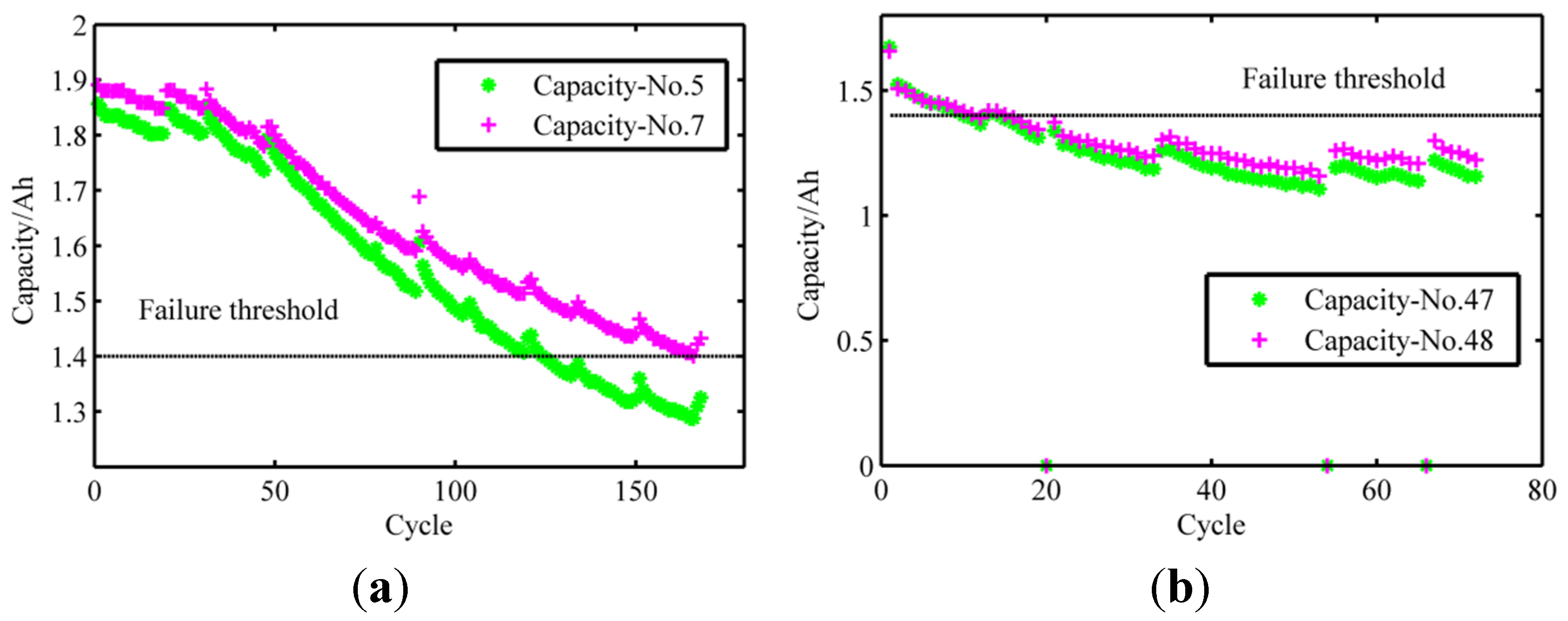
2.2. Capacity Degradation

The remaining capacity of a lithium-ion battery is influenced by many factors. Further, a lithium-ion battery does not undergo a complete charge process or a complete discharge process in actual operation. In this study, a typical charge and discharge process is regarded as a valuable cycle. It should be noted that the maximum capacity of the battery decreases with an increase in the battery working time [6] according to the current two sets of battery data. The battery capacity degradation for different discharging levels and different ambient temperatures is shown in Figure 1.
The measurements in Figure 1a were carried out at a constant current (CC) level of 2 A for Batteries Nos. 5 and 7 discharging at an ambient temperature of 24 °C; the measurements in Figure 1b were carried out at a CC level of 1 A to discharge Batteries Nos. 47 and 48 at an ambient temperature of 4 °C. Figure 1 shows that the battery capacity does not always decrease monotonically, but instead experience a sudden increase during the cycle. As an example, Figure 1a shows the capacity of different batteries increasing rapidly during the 90th cycle, resulting from self-charging [31] during the rest period. The explanation for this effect is that some chemical reactions occur during battery use, and some chemical products appear near the two electrodes, which retard the internal chemical reactions. Therefore, the battery needs a short rest period to melt these chemical products. The capacity of the battery increases suddenly owing to an increase in the available capacity in the next cycle. Figure 1 shows that the capacity degradation of the lithium-ion battery is regional; thus, the non-iterative prediction model is suitable for the F-SVR method. The F-SVR method will be detailed in Section 4.
Figure 1. Capacity degradation at different ambient temperatures of (a) 24 °C and (b) 4 °C.
Energies 07 06492 g001

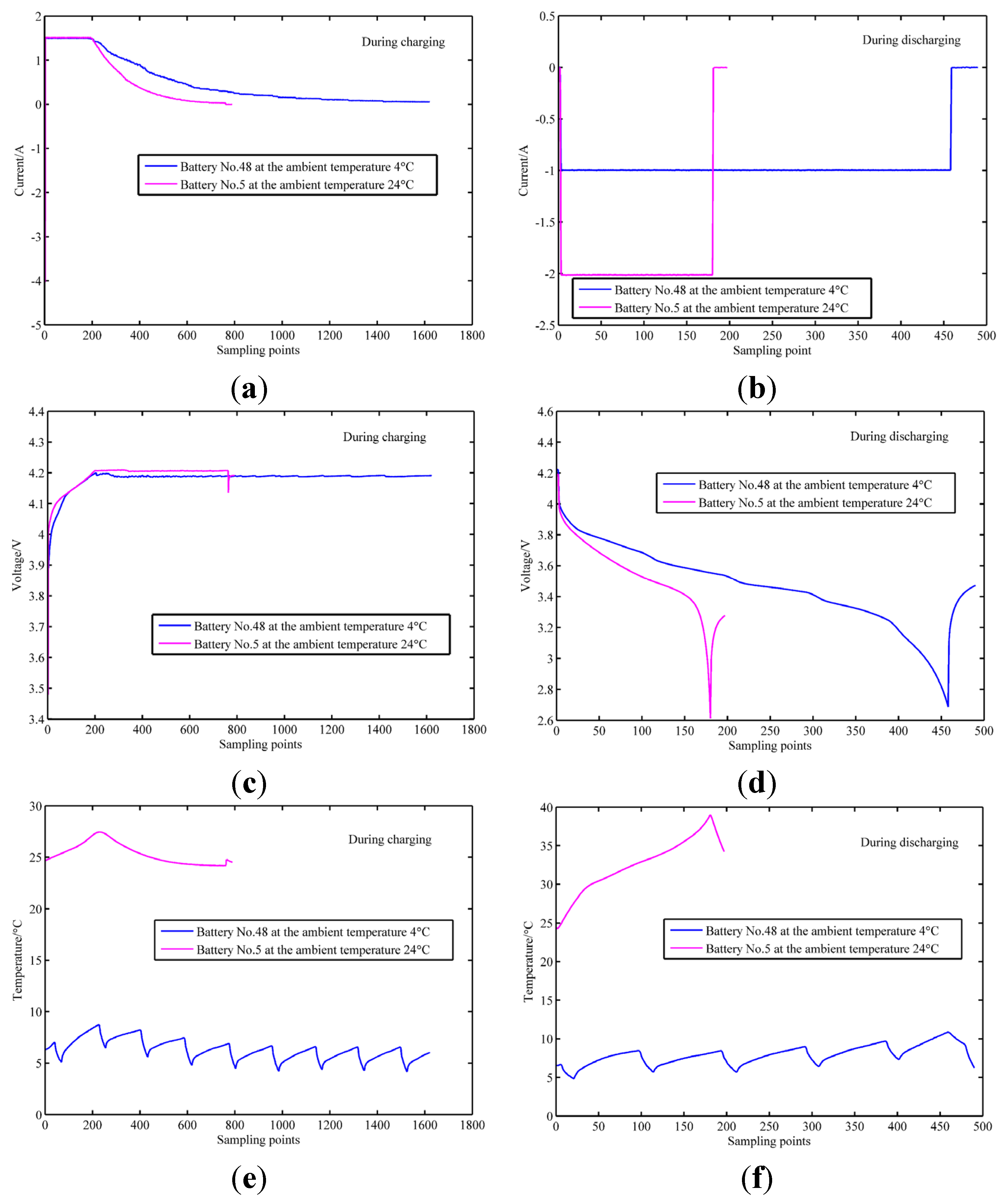
3. Energy Efficiency and Working Temperature

Current, voltage, and temperature have direct impacts on the battery capacity because of the nature of the battery mechanism and the electrochemical characteristics. The remaining capacity of a lithium-ion battery is influenced by many factors. Table 1 lists the symbols related to these parameters.
Table 1. Descriptions of symbols and acronyms.
SymbolsDescriptionSymbolsDescription
ICiCharge current in the ith cycleWCiCharge power in the ith cycle
IDiDischarge current in the ith cycleWDiDischarge power in the ith cycle
UCiCharge voltage in the ith cycleηiEnergy efficiency in the ith cycle
UDiDischarge voltage in the ith cycleCiThe capacity in the ith cycle
tCiCharge time in the ith cycleiCycle
tDiDischarge time in the ith cycleRULRemaining useful life
wtiTemperature in the ith cycleSVRSupport vector regression
TAmbient temperatureF-SVRFlexible support vector regression
btiWorking temperature in the ith cycleSSESum of squared errors
WPower of the batteryRMSERoot mean square error
The charging and discharging conditions for Batteries Nos. 5 and 48, respectively, from the data repository of the NASA Ames PCoE are shown in Figure 2.
Figure 2a,c,e shows the current, voltage, and temperature of Batteries Nos. 5 and 48 during the charging condition, respectively. Battery No. 5 is charged at an ambient temperature of 24 °C, in a CC mode at 1.5 A until the battery voltage reaches 4.2 V (190th sampling point), following which it continues to trickle charge [32]. Trickle charging means charging a fully charged battery under no-load at a rate equal to its self-discharge rate, thus enabling the battery to remain at its fully charged level. At the 230th sampling point, the battery temperature is at the highest position. At the same time, Battery No. 48 is charged at an ambient temperature of 4 °C until the battery voltage reaches 4.2 V (227th sampling point), following which it continues to trickle charge.
Figure 2b,d,f shows the current, voltage, and temperature of Batteries Nos. 5 and 48 during the discharging condition, respectively. Batteries Nos. 5 and 48, are discharged in a CC mode at 2 A. At the 180th and 459th sampling points for Batteries Nos. 5 and 48, respectively, the battery current is close to 0 A, the battery voltage reaches the lowest point, and the battery temperature is at its highest position. After the 180th and 459th sampling points, their temperatures decrease sharply, and their voltages increase slightly, which is called self-charging [33]. The ambient temperature is related to the battery capacity; therefore, the temperature should be used in the prediction models as the battery characteristic.
Figure 2. Charging and discharging conditions of Batteries No. 5 and 48: (a) current during charging; (b) current during discharging; (c) voltage during charging; (d) voltage during discharging; (e) temperature during charging; and (f) temperature during discharging.
Energies 07 06492 g002
In this paper, we define the input as a set comprising the charge current, discharge current, charge voltage, discharge voltage, charge time, discharge time, battery temperature, and ambient temperature, and we regard the capacity as the output space. In other words, we take the known quantities as the input space X = (ICi, IDi, UCi, UDi, tCi, tDi, wti, T), where there are some known relationships among these quantities as the following equations:
W = I × U × t
η i = W D i W C i   ×     1 00 %
bti = wtiT
Equation (1) shows the expression for electrical work that is the work done on a charged particle by an electric field. Three dimensions including current, voltage and time turn to only one dimension. Equation (2) is the definition of energy efficiency that the discharging electrical power divides by the charging electrical power during one valuable cycle. Equation (3) means that the working temperature is equal to the difference between battery temperature and ambient temperature. This is the actual temperature of the battery due to the operations. In addition, Equation (4) reduces two dimensions including battery temperature and ambient temperature by one dimension. Their relationships can reduce dimensions of input space and the computational complexity.
Therefore, there is a dimension reduction mapping Ø: R8R2:
Ø ( X ) = ( i = 0 I D i × U D i × t D i i = 0 I C i × U C i × t C i × 1 00 % ,   i = 0 ( w t i T ) i )
where i = 1, 2, 3 …. The first item of Equation (4) is the battery energy efficiency and the last item is the average working temperature according to Equations (1)–(3). The current methods establish prediction model using current, voltage, operation time, ambient temperature and so on. These current methods ignore the correlation of some performance metrics. Current, voltage and operation time jointly determine the physical performance called energy efficiency. Meantime, energy efficiency is closely related to the charge and discharge process of the battery. Therefore, we introduce energy efficiency as a key feature to predict the RUL of the lithium-ion batteries. In addition, the prediction models in this paper use energy efficiency and average working temperature as input data. These two physical quantities can not only preserve all the physical quantities (current, time, temperature and voltage) of the battery but also reduce the input dimensions (energy efficiency and average working temperature).

3.1. Energy Efficiency

Energy efficiency [17] is defined as the percentage of energy use which actually achieves the energy service required:
η = W D W C ×   100 %
where WD is the energy efficiency during discharging, and WC is the energy efficiency during charging. The energy efficiency of lithium-ion batteries reflects discharging and charging energy powers at the same cycle, so it is closely related to the battery capacity.

3.2. Working Temperature

Equation (3) indicates that the battery’s working temperature is the result of subtracting the ambient temperature from the battery temperature owing to the operation of the battery. Furthermore, the battery’s working temperature is composed of two parts: the charging temperature and the discharging temperature. In this paper, we define that the mapping of the battery temperature in Equation (4) represents the average working temperature as a scalar value for each cycle.

4. Prediction of the Remaining Useful Life for Lithium-Ion Batteries

In this study, we calculate the energy efficiency and average working temperature via computation with the original data, which reduces the dimensions of the input data. Then, we present a non-iterative prediction model and a multi-step prediction model using F-SVR [29] and SVR [14] theory, respectively, in the training process. The capacity degradation of the lithium-ion battery is regional; therefore, the non-iterative prediction model is suitable for the F-SVR method. The F-SVR method divides the training sample dataset into several regions according to the distribution complexity and then generates a different parameter set for each region, so it can accurately fit the RUL trend. The non-iterative prediction model provides the battery capacity forecasting results of all the cycles, whereas the multi-step prediction model forecasts the battery capacity of the next cycle, and the prediction results are obtained through data iteration, as shown in Figure 3.
Figure 3. Battery RUL prediction model based on energy efficiency and the average working temperature: (a) the non-iterative prediction model based on the F-SVR method; and (b) the iterative multi-step prediction model based on the SVR method.
Energies 07 06492 g003

4.1. Support Vector Regression

The support vector (SV) algorithm [34] is a nonlinear generalization of the generalized portrait algorithm developed by Vapnik [35] in the 1960s. SVR [14] adopts the original machine learning algorithm and applies it for non-parametric function estimation. Conventional SVR is formulated as a convex quadratic programming (QP) problem and has been successfully applied in identifying nonlinear dynamic systems. SVR is chosen for this study because of its excellent approximation and generalization capability and its demonstrated potential in the realm of nonlinear system identification.
We assume that we are given training data {(x1, y1), … , (xl, yl)} with unknown distribution function, the core technique for SVR is to find a proper parameter vector p0 and the optimal hyper-plane (the vector w0):
( p 0 , w 0 ) = arg min p , w : R S R M ( w , p ) = R E R M + ϕ ( w ) = arg min p , w : 1 l i = 1 l L o s s ( y i , f ( x i , w , p ) ) + 1 2 ( w w )
where Loss(yi, f(xi, w, p)) = (Ci|yi − ( i l βiK (x, y) + b)|ε, p: C, ε, K(·), C is the penalty parameter, ε is the insensitive parameter, K(·) is the kernel function, w is the weight vector, p is the regression parameter, βi is the Lagrange multiplier and |yi − ( i l βiK(x, xi) + b)|ε is the slack variable.

4.2. Flexible Support Vector Regression

Considering the penalty parameter C = c(xi), the insensitive parameter ε = g(xi), and the parameter for the RBF kernel width σ = s(xi) as flexible parameters, the following Lagrangian can be obtained to compute the regression using a direct development of Hao’s work [36]:
min : L ( α ) = 1 2 ( w , w ) +   c ( x i ) i = 1 l ( ξ i + ξ i * ) i = 1 l α i ( y i ( w , x i ) b + g ( x i ) + ξ i ) i = 1 l α i * ( y i + ( w , x i ) + b + g ( x i ) + ξ i * ) i = 1 l ( β i ξ i + β i * ξ i * )  
where:
ξ i = | y i ( i = 1 l β i | | x x i | | 2 2 s ( x i ) + b ) | g ( x i )
However, there are too many variables in this Lagrangian formula, and the optimization will require considerable computation which reduces its feasibility. Thus, F-SVR has partly combined the work of Cherkassky and Ma [37] and the idea of Hao’s variable parameters to set flexible parameters. The basic idea of the proposed F-SVR is that the training samples should be divided into several regions according to the distribution complexity, and different parameters should be set for different regions.
If the distribution is complicated, rigorous parameters should be set, on the other hand, slack parameters should be set. The F-SVR method is used to obtain a group of parameter sets p* = { p 1 * , p 2 * ,..., p k * } that can minimize the following formula:
R ( w , p ) = T 1 L ( y , f ( x , w , p 1 ) ) p ( x , y ) d x d y   +   T 2 L ( y , f ( x , w , p 2 ) ) p ( x , y ) d x d y   +   + T 3 L ( y , f ( x , w , p 3 ) ) p ( x , y ) d x d y
Equation (9) can be minimized by solving a QP problem. Therefore, we propose a flexible method to implement SVR, which divides the training samples into several regions and generates variable parameters in different regions. It replaces the fixed parameter set p: {ε, σ, C} with a group of adaptive parameter sets:
{ p * = { ( ε 1 , σ 1 , C 1 ) , ( ε 2 , σ 2 , C 2 ) , , ( ε k , σ k , C k ) } ε i = g 1 ( T i ) , σ i = g 2 ( T i ) , C i = g 3 ( T i )
where the training samples have been divided into k regions and where Ti and pi are the training samples and parameter set for the ith region, respectively. The significant of their work is the idea of flexibility: parameters should vary according to sample distribution but not as constants. However, only one of the three parameters was investigated in his paper, and in some cases, it is insufficient for practical application. Therefore, we propose a flexible method for SVR, which divides the training samples into several regions, and generates variable parameters in different regions. It replaces the fixed parameter set p: {ε, σ, C} with a group of adaptive parameter sets Equation (10).
The specific implementation process of F-SVR is as follows:
Step 1. Selecting SVs for each region: the samples have been divided into k regions with different CP values which are used to measure the distribution complexities. In addition, a suitable set of parameters p is given for each region according to the CP value. As mentioned above, the selected parameter p determines which samples should be picked up as SVs.
Step 2. Selecting a new training set: if TSi is the selected SV for the ith region, we obtain the new training set SVs = {TS1, TS2, …, TSk} = { S V j } j = 1 m .
Step 3. Selecting the function approximation: according to Equation (11), the regression could be managed by approximating the unknown function of the new training set which is composed of all SVs:
f ( x ) = i = 1 m γ i K ( x , S V i ) + γ 0
Generally, a large value for k may lead to more reasonable choosing of SVs but also causes a significant increase in computing time. There exists a trade-off between the computing time and the k regions. In many cases, a setting of 1 ≤ k ≤ 5 is more than enough. CP is the complexity estimating function. S is the function to evaluate the quality of the sample division. If the training samples have been divided into k regions, the complexity for each region is CPi = 1, 2, …, k.
The SVR method aims to obtain the global optimal fitting results from the total training data. This method is more suitable for short-term or medium-term prediction and real-time monitoring systems. Because the SVR can obtain the optimal one-step prediction, we can adopt a period of data to obtain the predictive results. However, the F-SVR method aims to obtain the local optimal fitting results from the original data that divide the training sample into several regions according to the distribution complexity of all data. In this way, the F-SVR method will generate different parameters for each sub-dataset; thus, it is suitable for predicting the whole trend.
In the prediction models presented in this paper, we set k1 and k2 as 3 and 2, respectively, according to Figure 1. The capacities of Batteries No. 5 and 7 increased rapidly at the 48th and the 90th cycle, whereas the capacities of Batteries Nos. 47 and 48 increased rapidly at the 14th cycle, resulting from self-charging during the rest period. Figure 1b shows that the capacity decreased rapidly and reached the EOL at the 16th cycle. Therefore, we only consider 29 cycles and k2 = 2 is more than enough for Batteries Nos. 47 and 48. Figure 4 presents the regions of capacity at different ambient temperatures.
Figure 4. Regions of the capacity at different ambient temperature of (a) 24 °C and (b) 4 °C.
Energies 07 06492 g004

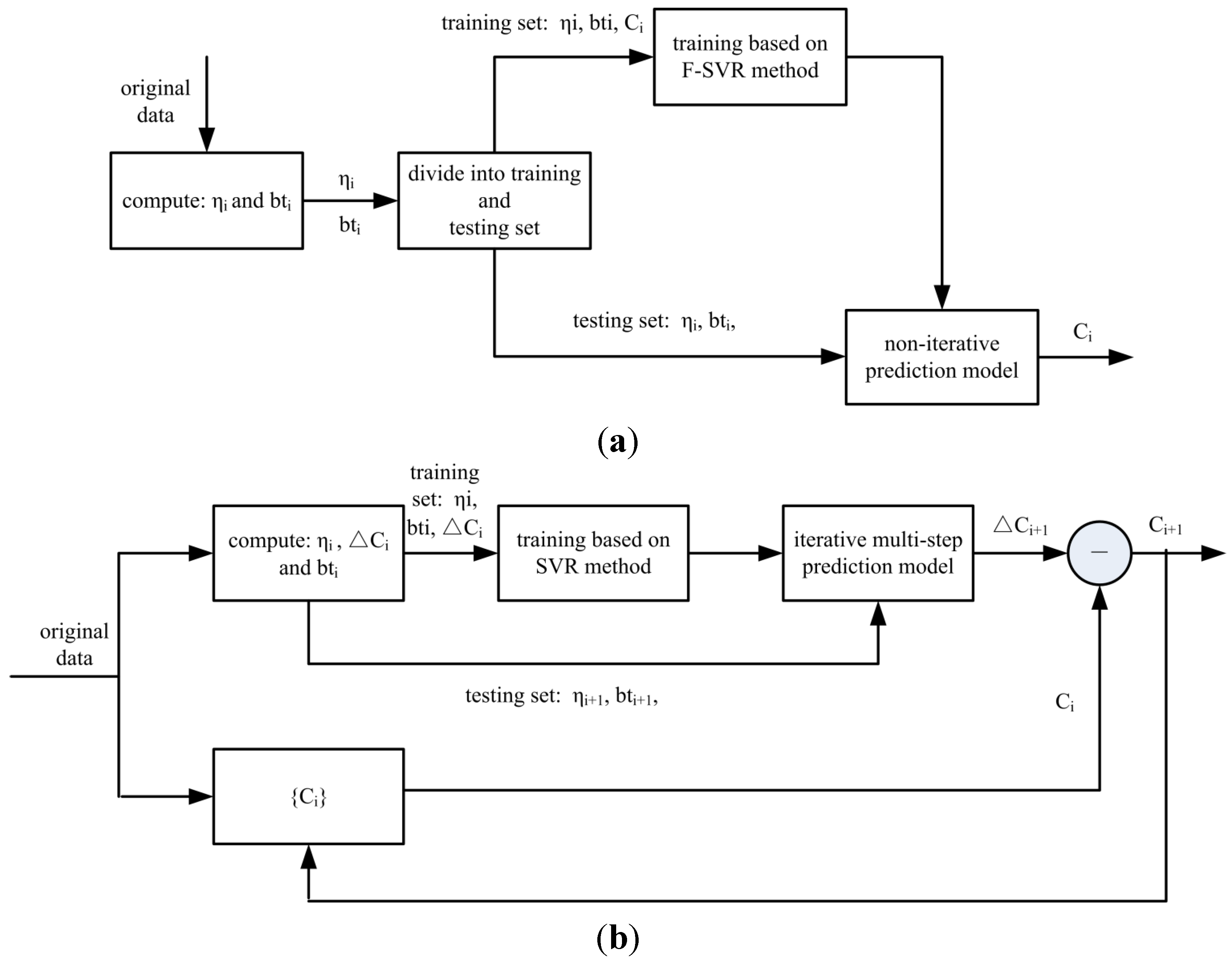
4.3. Non-Iterative Prediction Model

The non-iterative prediction model is used to consider the influence of the energy efficiency and the average working temperature on the remaining capacity. This model uses the known ith cycle energy efficiency ηi and the average working temperature bti to forecast the ith cycle battery capacity as follows:
Ci = hi,bti)
The battery data for charging at a CC level of 2 A, at an ambient temperature of 24 °C, have been divided into three regions on the basis of the F-SVR concept, as shown in Figure 4a. Therefore, the non-iterative prediction model at an ambient temperature of 24 °C can be described as follows:
C i = { h 1 ( η i , b t i )         1 i 47 h 2 ( η i , b t i )         48 i 89 h 3 ( η i , b t i )               9 0 i 168
The battery data for charging at a CC level of 2 A and an ambient temperature of 24 °C, have been divided into three regions. Because the battery capacity degradation of Batteries Nos. 47 and 48 is rapid as shown in Figure 1b, and the capacity exhibits complex behavior after reaching the failure threshold, we only consider 29 cycles for Batteries Nos. 47 and 48 as shown in Figure 4b. Figure 4b shows that only the T1 and T2 region can be used for making predictions. Therefore, the non-iterative prediction model at an ambient temperature of 24 °C can be described as follows:
C i = { h 4 ( η i , b t i )           1 i 11 h 5 ( η i , b t i )         12 i 29

4.4. Iterative Multi-Step Prediction Model

It should be noted that the maximum available capacity decreases with an increase in the battery working time. The iterative multi-step prediction model is used to predict the capacity of the next cycle from the capacities of the previous cycles, and it is then used to obtain extrapolation forecasting results after multiple iterations. A lithium-ion battery does not undergo a complete charge process or a complete discharge process in actual operation; therefore, ηi and bti for each cycle have an impact on the capacity variation as follows:
ΔCi = zi,bti)
The battery capacity variation is the difference between the remaining battery capacity of a given cycle and that of the next cycle:
ΔCi = Ci−1Ci
Therefore, the iterative multi-step prediction model can be described as follows:
Ci = Ci−1Ci

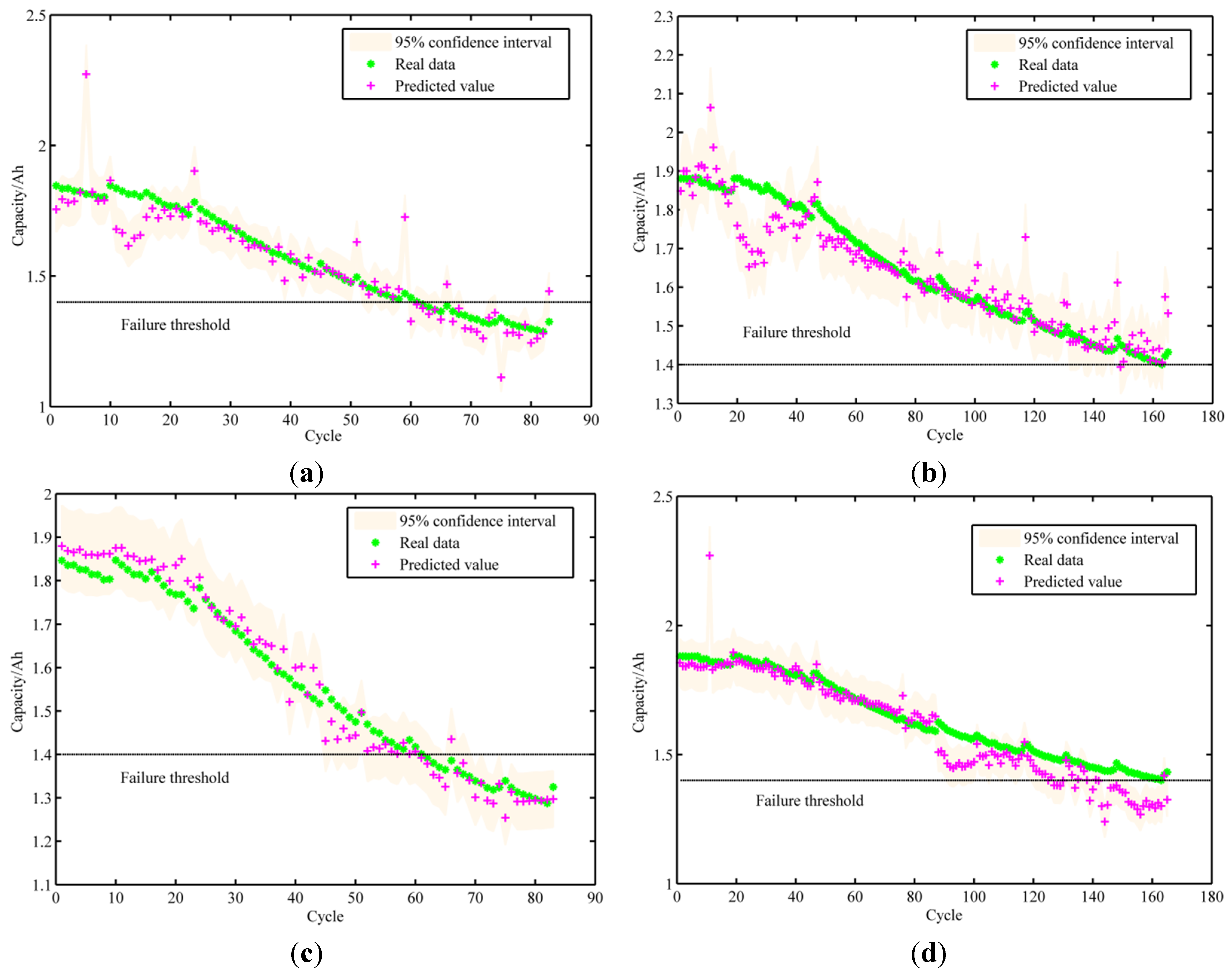
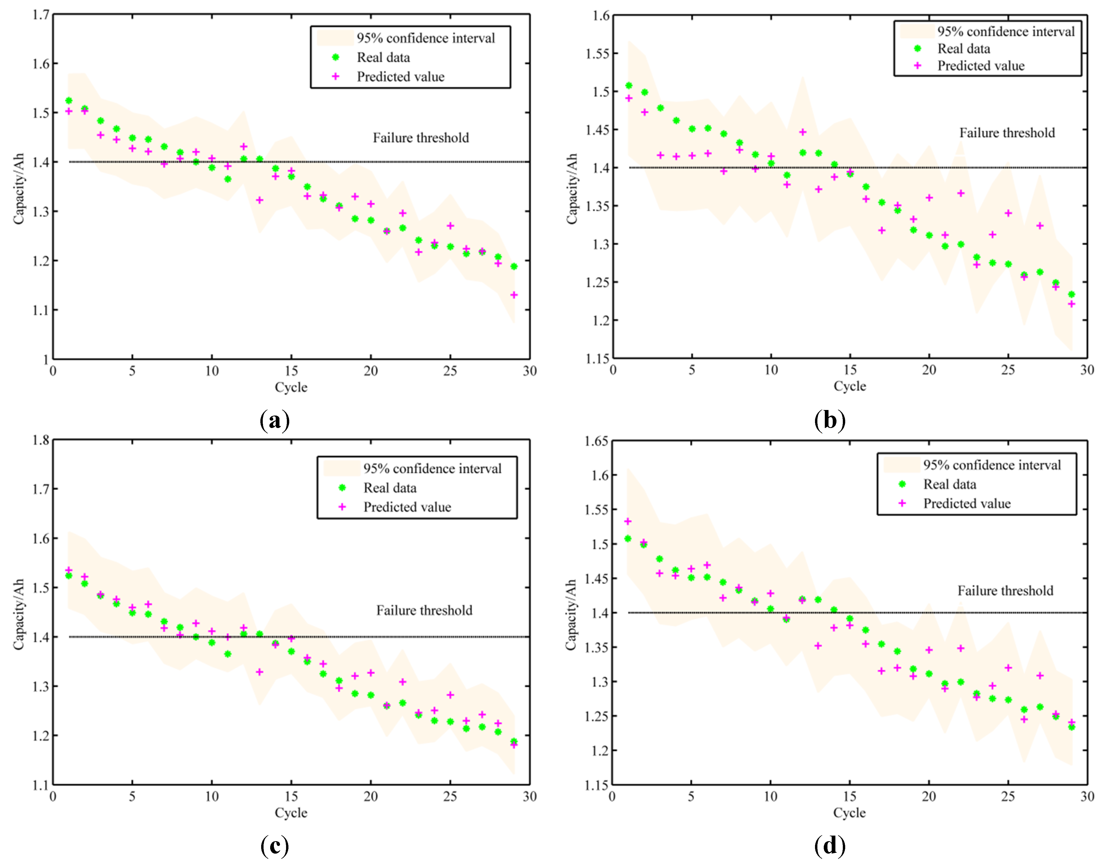
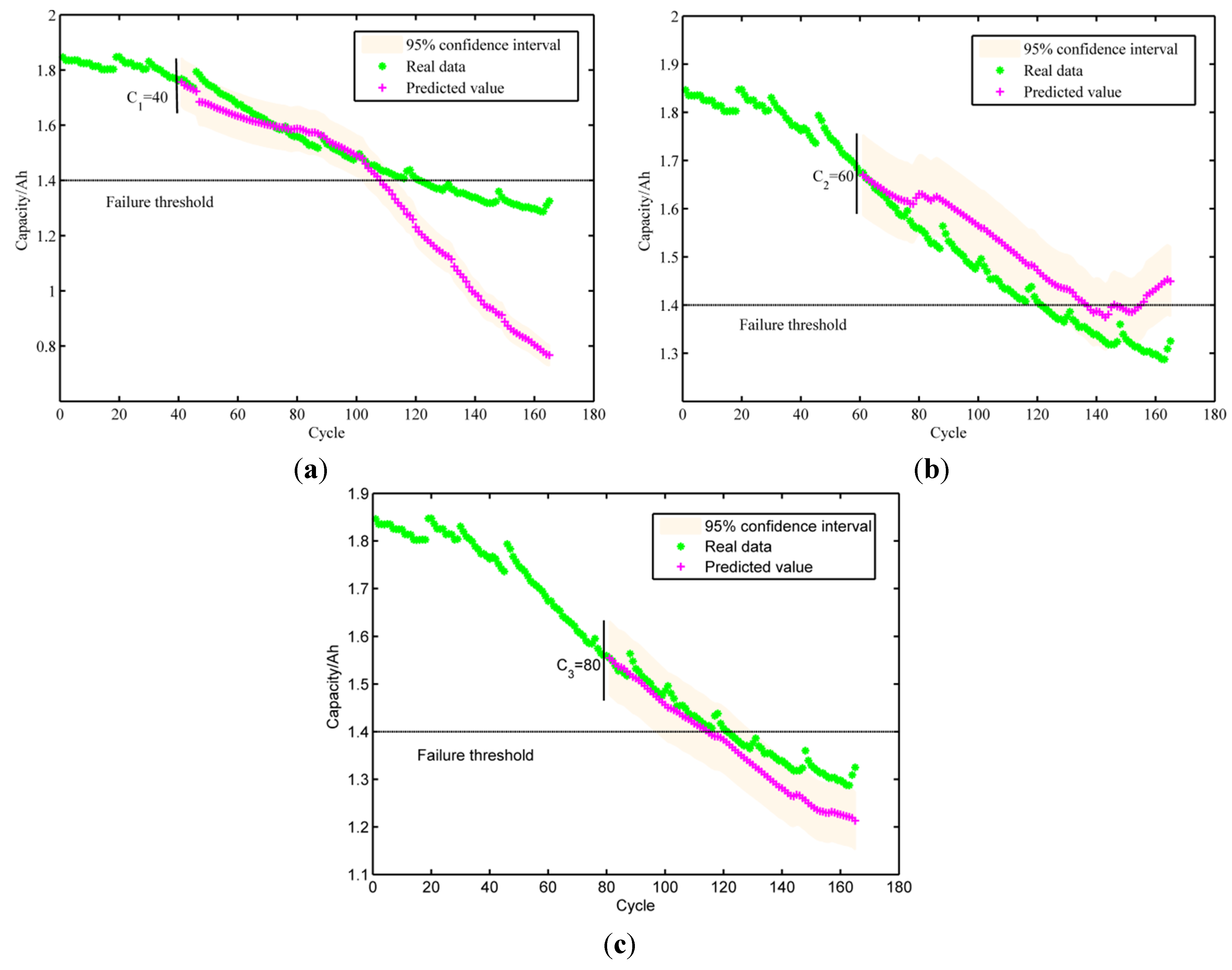
5. Prognostic Results and Discussion

In the experiment, we adopt the sum of squared errors (SSE), the root mean square error (RMSE), and the RUL estimate error to analyze the prediction results and quantitatively evaluate the comparison results. The SSE is the sum of the squared differences between each observation and its group’s mean and can be used as a measure of the variation within a cluster. The formula for the SSE is given as follows:
S S E = i = 1 n ( y ̂ i y i ) 2
The RMSE gives the standard deviation of the model prediction error. A smaller value indicates better model performance. The formula for the RMSE is given as follows:
R M S E = 1 n i = 1 n ( y ̂ i y i ) 2
The RUL estimate error is the absolute value of the difference between the number of real cycles and the predicted number of cycles. The formula for the RUL estimate error is given as follows:
E R U L = | R U L real R U L prediction |
This section presents the experimental results of the two proposed models. According to distribution complexity of different samples, the real value of parameter is a certain probability to be around the certain rang. In this paper, we think that all the parameters are normal distribution. In the first case, the data of Battery No. 5’s even-number cycles are used for training to obtain the parameters of the prediction model with Equations (13) and (14). The data of Battery No. 5’s odd-number and No. 7’s cycles are for testing. Because the capacities of Batteries Nos. 47 and 48 decrease sharply and their lifetimes are short, the data for Batteries Nos. 47 and 48 are used to train and test. The detailed results are shown in Figure 5 and Figure 6 and Table 2.
Figure 5. Comparison between the results obtained from the results of the SVR and F-SVR methods at an ambient temperature of 24 °C. Predictive results of the SVR method for: (a) Battery No. 5’s odd-number cycles; and (b) Battery No. 7. Predictive results of the F-SVR method for: (c) Battery No. 5’s odd-number cycles; and (d) Battery No. 7.
Energies 07 06492 g005
The experimental results show that the F-SVR method can more accurately fit the RUL trend than the SVR method. The predicted values for Battery No. 7 in the T3 region with the F-SVR method are not accurate with respect to the real data because Battery No. 7 does not reach the EOL, and its capacity slowly degrades.
Figure 6. Comparison between the results obtained from the results of the SVR and F-SVR methods at an ambient temperature of 4 °C. Predictive results of the SVR method for: (a) Battery No. 47; and (b) Battery No. 48. Predictive results of the F-SVR method for: (c) Battery No. 47; and (d) Battery No. 48.
Energies 07 06492 g006
Table 2. Comparisons between the results obtained from the SVR and F-SVR methods for predicting the RULs of different batteries.
BatteryMethodSSERMSEReal cyclePredictive cycleERUL
No. 5’s odd-number cycleSVR0.63780.039462602
F-SVR0.12500.023162611
No. 7SVR0.62160.02021681680
F-SVR0.86420.040716815018
No. 47SVR0.03690.00971073
F-SVR0.03370.009910111
No. 48SVR0.04730.00501192
F-SVR0.03180.006911110
In the second case, the forecasts of the RUL of a lithium-ion battery are not significant because the battery degrades sharply and the short lifetime is at a low temperature. Thus, the data from Battery No. 5’s current states are used to determine the iterative multi-step prediction model parameters by using Equations (16) and (17), whereas Battery No. 5 is used for testing to show the capacity fading trend compared to the forecast at 40, 60, and 80 cycles due to Battery No. 7 not reaching the EOL. The detailed results are shown in Figure 7 and Table 3. The experimental results show that the RUL estimate error decreases with an increase in the number of cycles.
Figure 7. RUL estimation based SVR method for Battery No. 5 at different starting points: (a) at the 40th point; (b) at the 60th point; and (c) at the 80th point.
Energies 07 06492 g007
Table 3. Comparisons at different starting points for predicting the RUL of Battery No. 5.
ith cycleSSERMSEReal CyclePredictive CycleERUL
40th cycle6.76490.115012411212
60th cycle0.67190.021012414016
80th cycle0.28070.03001241186
From the above discussion, we concluded that the working temperature has some effects on the RUL of lithium-ion batteries and the energy efficiency is related to the RUL of lithium-ion batteries. Thus, it is feasible to develop a lifetime prediction model for lithium-ion batteries on the basis of the energy efficiency and working temperature.

6. Conclusions

A lithium-ion battery will decrease in capacity over repeated charge and discharge cycles which may lead to failure of a battery even catastrophic failure. Accurate prediction of the RUL of a lithium-ion battery is of vital importance. From the analysis of the lithium-ion battery data, we use the energy efficiency and working temperature as the input data of the proposed models. In contrast with other methods, the proposed method considers the effects of all the performance metrics of a lithium-ion battery on the RUL and the relationships between each performance metric. The non-iterative prediction model based on F-SVR is suitable for long-term prediction, whereas the iterative multi-step prediction model based on SVR is suitable for short-term or medium-term prediction and real-time monitoring systems.
The following contributions of this study include:
(1)
the energy efficiency and the battery working temperature are used as input physical characteristics of the two proposed models;
(2)
the energy efficiency is found to be closely related to the capacity of the lithium-ion battery;
(3)
a non-iterative prediction model based on the F-SVR method is proposed;
(4)
an iterative multi-step prediction model based on the SVR method is proposed.
Our future work includes estimation of the RUL of the lithium-ion battery using the energy efficiency. Furthermore, the current linear prediction model has a one-step prediction value; therefore, further research should be focused on modifying the linear model with the energy efficiency and obtaining more accurate nonlinear iterative multi-step prediction.

Acknowledgments

The authors would like to extend their sincere thanks to the NASA Ames Laboratory for providing open data.

Conflicts of Interest

The authors declare no conflict of interest.

References

  1. He, Z.; Gao, M.; Wang, C.; Wang, L.; Liu, Y. Adaptive state of charge estimation for Li-ion batteries based on an unscented Kalman filter with an enhanced battery model. Energies 2013, 6, 4134–4151. [Google Scholar] [CrossRef]
  2. Liu, D.; Wang, H.; Peng, Y.; Xie, W.; Liao, H. Satellite lithium-ion battery remaining cycle life prediction with novel indirect health indicator extraction. Energies 2013, 6, 3654–3668. [Google Scholar] [CrossRef]
  3. Zhang, J.; Lee, J. A review on prognostics and health monitoring of Li-ion battery. J. Power Source 2011, 196, 6007–6014. [Google Scholar] [CrossRef]
  4. Liaw, B.Y.; Jungst, R.G.; Nagasubramanian, G.; Case, H.L.; Doughty, D.H. Modeling capacity fade in lithium-ion cells. J. Power Source 2005, 140, 157–161. [Google Scholar] [CrossRef]
  5. Xing, Y.; Ma, E.W.M.; Tsui, K.L.; Pecht, M. Battery management systems in electric and hybrid vehicles. Energies 2011, 4, 1840–1857. [Google Scholar] [CrossRef]
  6. Williard, N.; He, W.; Hendricks, C.; Pecht, M. Lessons learned from the 787 Dreamliner issue on lithium-ion battery reliability. Energies 2013, 6, 4682–4695. [Google Scholar] [CrossRef]
  7. Chen, Y.; Miao, Q.; Zheng, B.; Wu, S.; Pecht, M. Quantitative analysis of lithium-ion battery capacity prediction via adaptive bathtub-shaped function. Energies 2013, 6, 3082–3096. [Google Scholar] [CrossRef]
  8. Jin, G.; Matthews, D.E.; Zhou, Z. A Bayesian framework for online degradation asseeement and residual life prediction of secondary batteries inspacecraft. Reliab. Eng. Syst. Saf. 2013, 113, 7–20. [Google Scholar] [CrossRef]
  9. Xing, Y.; Ma, E.W.M.; Tsui, K.L.; Pecht, M. An ensemble model for predicting the remaining useful performance of lithium-ion batteries. Microelectron. Reliab. 2013, 53, 811–820. [Google Scholar] [CrossRef]
  10. Wang, X.X.; Ma, L.Y. A compact K nearest neighbor classification for power plant fault diagnosis. J. Inf. Hiding Multimed. Signal Process. 2014, 5, 508–517. [Google Scholar]
  11. Zhang, Q.; White, R.E. Capacity fade analysis of a lithium ion cell. J. Power Source 2008, 179, 793–798. [Google Scholar] [CrossRef]
  12. Liu, D.; Pang, J.; Zhou, J.; Peng, Y.; Pecht, M. Prognostics for state of health estimation of lithium-ion batteries based on combination Gaussian process functional regression. Microelectron. Reliab. 2013, 53, 832–839. [Google Scholar] [CrossRef]
  13. Groot, J. State-of-Health Estimation of Li-Ion Batteries: Cycle Life Test Methods; Chalmers University of Technology: Göteborg, Sweden, 2012. [Google Scholar]
  14. Weng, C.; Cui, Y.; Sun, J.; Peng, H. On-board state of health monitoring of lithium-ion batteries using incremental capacity analysis with support vector regression. J. Power Source 2013, 235, 36–44. [Google Scholar] [CrossRef]
  15. Le, D.; Tang, X. Lithium-ion battery state of health estimation using Ah-V characterization. In Proceedings of the Annual Conference of Prognostics and Health Management (PHM) Society, Montreal, QC, Canada, 25–29 September 2011; pp. 367–373.
  16. Tang, S.; Yu, C.; Wang, X.; Guo, X.; Si, X. Remaining useful life prediction of lithium-ion batteries based on the wiener process with measurement error. Energies 2014, 7, 520–547. [Google Scholar] [CrossRef]
  17. Miao, Q.; Xie, L.; Cui, H.; Liang, W.; Pecht, M. Remaining useful life prediction of lithium-ion battery with unscented particle filter technique. Microelectron. Reliab. 2013, 53, 805–810. [Google Scholar] [CrossRef]
  18. Si, X.S.; Wang, W.; Hu, C.H.; Zhou, D.H. Remaining useful life estimation—A review on the statistical data driven approaches. Eur. J. Oper. Res. 2011, 213, 1–14. [Google Scholar] [CrossRef]
  19. Chen, C.; Pecht, M. Prognostics of lithium-ion batteries using model-based and data-driven methods. In Proceedings of the 2012 IEEE Conference on Prognostics and System Health Management (PHM), Beijing, China, 23–25 May 2012; pp. 1–6.
  20. Fan, Z.; Liu, G.; Si, X.; Zhang, Q. Degradation datadriven approach for remaining useful life estimation. J. Syst. Eng. Electron. 2013, 24, 173–182. [Google Scholar] [CrossRef]
  21. Nuhic, A.; Terzimehic, T.; Soczka-Guth, T.; Buchholz, M.; Dietmayer, K. Health diagnosis and remaining useful life prognostics of lithium-ion batteries using data-driven methods. J. Power Source 2013, 239, 680–688. [Google Scholar] [CrossRef]
  22. Long, B.; Xian, W.; Jiang, L.; Liu, Z. An improved autoregressive model by particle swarm optimization for prognostics of lithium-ion batteries. Microelectron. Reliab. 2013, 53, 821–831. [Google Scholar] [CrossRef]
  23. Fleischer, C.; Wang, W.; Bai, Z.; Sauer, D.U. On-line self-learning time forward voltage prognosis for lithium-ion batteries using adaptive neuro-fuzzy inference system. J. Power Source 2013, 243, 728–749. [Google Scholar] [CrossRef]
  24. Chang, W.Y. Estimation of the state of charge for a LFP battery using a hybrid method that combines a RBF neural network, an OLS algorithm and AGA. Int. J. Electr. Power Energy Syst. 2013, 53, 603–611. [Google Scholar] [CrossRef]
  25. Zheng, Y.; Ouyang, M.; Lu, L.; Li, J.; Han, X.; Xu, L. On-line equalization for lithium-ion battery packs based on charging cell voltages: Part 2. Fuzzy logic equalization. J. Power Source 2014, 247, 460–466. [Google Scholar] [CrossRef]
  26. Álvarez Antón, J.; García Nieto, P.; Blanco Viejo, C.; Vilán Vilán, J. Support vector machines used to estimate the battery state-of-charge. IEEE Trans. Power Electron. 2013, 28, 5919–5926. [Google Scholar] [CrossRef]
  27. Wang, D.; Miao, Q.; Pecht, M. Prognostics of lithium-ion batteries based on relevance vectors and a conditional three-parameter capacity degradation model. J. Power Source 2013, 239, 253–264. [Google Scholar] [CrossRef]
  28. Xing, Y.; He, W.; Pecht, M.; Tusi, K.T. State of charge estimation of lithium-ion batteries using the open-circuit voltage at various ambient temperatures. Appl. Energy 2014, 113, 106–115. [Google Scholar] [CrossRef]
  29. Yi, H.; Song, X.F.; Jiang, B.; Liu, Y.F.; Zhou, Z.H. Flexible support vector regression and its application to fault detection. Acta Autom. Sin. 2013, 39, 272–284. [Google Scholar] [CrossRef]
  30. Saha, B.; Goebel, K. Battery Data Set; National Aeronautics and Space Administration (NASA) Ames Prognostics Data Repository: Moffett Field, CA, USA, 2007. [Google Scholar]
  31. Xue, X.; Wang, S.; Guo, W.; Zhang, Y.; Wang, Z.L. Hybridizing energy conversion and storage in a mechanical-to-electrochemical process for self-charging power cell. Nano Lett. 2012, 12, 5048–5054. [Google Scholar] [CrossRef] [PubMed]
  32. Lin, D.S.; Perkins, P.; Schneider, M.E. Pulse Charge Technique to Trickle Charge a Rechargeable Battery. U.S. Patent 5,539,298, 23 July 1996. [Google Scholar]
  33. Zhang, W.; Duan, D.; Yang, L. Relay selection from a battery energy efficiency perspective. In Proceedings of the IEEE MILCOM 2009 on Military Communications Conference, Boston, MA, USA, 18–21 October 2009; pp. 1–7.
  34. Smola, A.J.; Schölkopf, B. A tutorial on support vector regression. Stat. Comput. 2004, 14, 199–222. [Google Scholar] [CrossRef]
  35. Vapnik, V. The Nature of Statistical Learning Theory; Springer-Verlag: Berlin, Germany, 1995. [Google Scholar]
  36. Hao, P.Y. New support vector algorithms with parametric insensitive/margin model. Neural Netw. 2010, 23, 60–73. [Google Scholar] [CrossRef] [PubMed]
  37. Cherkassky, V.; Ma, Y. Practical selection of SVM parameters and noise estimation for SVM regression. Neural Netw. 2004, 17, 113–126. [Google Scholar] [CrossRef] [PubMed]

