Optimal Time to Invest Energy Storage System under Uncertainty Conditions

Abstract

This paper proposes a model to determine the optimal investment time for energy storage systems (ESSs) in a price arbitrage trade application under conditions of uncertainty over future profits. The adoption of ESSs can generate profits from price arbitrage trade, which are uncertain because the future marginal prices of electricity will change depending on supply and demand. In addition, since the investment is optional, an investor can delay adopting an ESS until it becomes profitable, and can decide the optimal time. Thus, when we evaluate this investment, we need to incorporate the investor's option which is not captured by traditional evaluation methods. In order to incorporate these aspects, we applied real option theory to our proposed model, which provides an optimal investment threshold. Our results concerning the optimal time to invest show that if future profits that are expected to be obtained from arbitrage trade become more uncertain, an investor needs to wait longer to invest. Also, improvement in efficiency of ESSs can reduce the uncertainty of arbitrage profit and, consequently, the reduced uncertainty enables earlier ESS investment, even for the same power capacity. Besides, when a higher rate of profits is expected and ESS costs are higher, an investor needs to wait longer. Also, by comparing a widely used net present value model to our real option model, we show that the net present value method underestimates the value for ESS investment and misleads the investor to make an investment earlier.

1. Introduction

Nowadays, in the era of energy shortage, the development of energy storage systems (ESSs) has been highlighted because they can allow current and/or future power grids to operate more efficiently and can maximize its economic value [1,2]. In an electrical power grid, utility firms generate electricity continuously and balance electricity demand and supply. However, the demand for electricity fluctuates a lot over time and the generation capacity has to be set to the highest level of demand for maintaining electricity supply stability. This costs a huge investment in excess generators. For this reason, utility firms have been eager to lower the peak time demand and attract off-peak time consumption instead. Nowadays, incorporation of ESSs enables accomplishing such demand-smoothing by allowing customers to store electricity during off-peak times and use it during peak times. Besides, the reserve capacity enables arbitrage trade by selling during peak time unconsumed electricity which has been stored during off-peak times, which would be another source of profit. Also, the integration of renewable energy sources such as wind and solar provides generator stability, and support for frequency regulation, for spinning reserve capacity, for transmission and distribution, and for voltage including reactive power compensation allow grid reliability. For all these benefits of ESS utilization, several studies have recently investigated if investment in ESSs is economically viable or not [1,3], and extensive efforts have been made to evaluate economic profitability of ESSs [1,4–6].

However, two very important aspects have been disregarded in this investment evaluation, which are a firm's options and the uncertainty of future profits. Despite its many benefits, if the investment is not profitable at a certain point in time, the firm will not invest and rather wait until the cost of the ESS decreases or the profit from the ESS will increase. In other words, the utility firm has decision flexibility in its investment, which can be called an option. Moreover, the firm faces uncertainty in the profit structure. Specifically, in an arbitrage trade that profits by selling electricity at a high price during peak time which has been charged at a low price, the market prices are determined by demand and supply in a market which is affected by many uncertain factors, therefore, the future profits from the trade will be uncertain as well. Moreover, even though the electricity price pattern for the same time period every year might be similar, we need to note that the price values might be different and the profits from the trade are uncertain. For example, the price pattern in March 2014 may be similar to that in March 2015, but the value of the former may be not exactly the same as the value of the latter. Therefore, the consideration of uncertainty is inevitable. However, previous studies fail to discuss these two factors simultaneously. Some studies related to evaluation of ESS investment like [1,3] did not take uncertainty into account. Also, even though the most recent research [2] emphasizes the importance of unavoidable uncertainty, an option to determine when to invest is not considered.

State-of-the-art economics literature in the general economic analysis area has suggested a novel approach for investment evaluation under uncertainty and decision flexibility conditions [7–10], which is a real option approach. The reason that this approach is important is that the results obtained when using a real option method and classical investment evaluation methods, such as net present value (NPV) method and internal rate of return (IRR), are significantly different when a firm can determine when to invest under uncertainty conditions. Compared to classical methods, the real option theory is considered more accurate when a firm has an option to delay investment, because it can capture the value of the postponement which is called decision flexibility. In our problem, ESS investment is not an obligation but an option to a firm, because the firm can delay the ESS investment in order to maximize profits. Besides, the real option theory has an advantage of being able to give an optimal time to invest, in contrast to classical methods. Therefore, in this paper, we applied the real option theory to obtain a more accurate investment evaluation and optimal time. In energy areas, the real option approach was recently applied in renewable energy, electricity markets, and power system evaluations [11–15], but not in energy storage investment.

Thus, in this research we discuss how decision-making might be different under uncertainty and decision flexibility. We focus specifically on investment in the arbitrage trade application of ESSs. However, we need to note that the proposed model can be extended easily to other ESS applications. The structure of this paper is as follows: in Section 2, we intensively investigate the literature regarding ESS investment and real option theory. Then, we develop a new model for ESS investment evaluation in Section 3. Based on the proposed model, simulation and analysis are executed to examine how the investment decision changes due to uncertainty, option and other important environmental factors in Section 4. Section 5 summarizes the major results, and provides implications for power system management and future research.

2. Literature Review and Methodology

An energy storage system (ESS) is a storage device which allows one to charge and discharge electricity in a very short time. Since it has lots of benefits in areas such as load-shifting, reliability, stabilization of power grids, utility firms have come to pay attention to the utilization of ESSs. Depending on the purpose of the ESS, its power and storage capacity specifications can be different, but basically ESS provides different types of profits by repeating charge and discharge during its lifetime. For example, Sandia Lab [16] reports that ESSs derive 26 benefits like energy time-shift, regulation, voltage service, reliability, facility upgrade deferral, asset utilization increment, loss avoidance, etc., for 17 application areas such as electric supply, ancillary service, grid system, end use, and renewable integration. Similarly, those kinds of benefits are categorized into bulk energy services, ancillary services, transmission infrastructure services, distribution services, and customer energy management services and stacked services [17]. Likewise, the benefit of ESSs can be grouped into energy market, voltage control, power flow management, restoration, commercial/regulatory, and network management [18]. Among those benefits, several recent studies have started to focus on energy arbitrage trade in an energy market [1,3,19,20], because an ESS could be actively used in a future grid environment like a smart grid. In this sense, [19] analyzed the arbitrage value using PJM data to investigate the impact of fuel prices, transmission constraints, efficiency, storage capacity, and fuel mix. Also, similar research for the New York and U.S. markets has been done in [1,3]. Especially, [1] investigated the optimal policies of ESS storage capacity by applying internal rate of return (IRR) as an investment problem. In the stream of this research, in this paper we will discuss an evaluation model for price arbitrage trade that makes profits by selling electricity at a high price during peak times which has been charged at low price during off-peak times.

However, investment decision making problems in the aforementioned literature have not focused on when is the optimal time to invest, but rather have focused on whether or not it is feasible only at a decision making time. While the latter is related to determining a yes or no decision, the former is a decision regarding now or later if it is not feasible now. This implies that the firm has an option or decision flexibility about determining the optimal investment time. For example, in case of ESS investment, a firm may estimate profits and costs, and then calculate a net present value discounting the future cash flows. Under a classical net present value (NPV) method, a firm should give up a project if the net present value of the project is less than 0. By contrast, a real option theory reflects on the idea that, since a firm can determine when to invest and wants to maximize their profits, the firm will compare the investment values at a certain time and at the other time and then will choose a more profitable time. Of course, it is very clear that this approach is more realistic. Besides, we need to note that more important thing in investment is the fact that uncertainty is not ignorable or sometimes it is very crucial because it causes the decision flexibility, as described in economics literature [7]. However, only few studies about uncertainty in ESS investment became discussed [2,21]. In the case of price arbitrage trade, since the market price is determined by supply and demand which are uncertain, a firm encounters uncertain future cash flows from the utilization of ESS. In this environment, our proposed model in this paper will consider both uncertainty and option to determine an optimal investment time of the ESS for price arbitrage trade, by applying a novel evaluation method which is a real option approach.

The real option theory has been widely used to quantify decision flexibility under uncertainty ([22–25]). References [22,25,26] showed that a real option approach is very appropriate to model valuation of a project under uncertainty. In [7] the authors pointed out the similarities between the investment opportunities and perpetual American options, and found that the existence of opportunity costs can influence decision-making behavior. In the case of ESS investment, future cash flow from price arbitrage trade is not fixed and is uncertain over time. Also, a utility firm has an option for ESS investment, because it does not necessarily have to invest right now and can wait and delay the investment. Because losing the option to wait could expose the investor under a potential loss of money [27,28], it is commonly agreed in financial economics that no exercise of investment should take place unless its net profits at least compensate for the loss of “value of waiting” [29]. In contrast, a classical investment evaluation method, net present value (NPV) method, cannot capture the loss of value of waiting. For this reason, several recent papers such as [11–15,21] in the energy area have studied these topics. Nevertheless, real option model for ESS investment has not been paid attention yet. Therefore, in this paper, we develop a valuation model for arbitrage trade in order to determine when to optimally invest while considering uncertainty and decision flexibility. Then, we study the impacts of several important factors such as efficiency of discharging and volatilities as in [1,21].

3. Valuation Model

In this section, we develop a valuation model for when an energy storage system (ESS) is utilized for the purpose of arbitrage trade. As described in [1], the energy storage system can be characterized in terms of storage and power capacity, efficiency, and loss. Herein, storage capacity is the maximum amount that a storage device can hold and power capacity is the rate at which energy can be stored in and discharged out. Efficiency implies round trip efficiency and depth of discharge and the loss of energy is incurred due to technology limitations. However, in our model, both efficiency and loss can be comprehensively referred to as efficiency from the perspective of charging and discharging.

If energy storage system is installed, electricity can be stored in it during some time period and then the stored electricity will be discharged into a market. To model this arbitrage trade, let us assume π(τ) is the marginal price function, and Q(τ) is the function of amount of electricity or the power capacity. Also, let us assume that the ESS operator charges from time T_CS to T_CS + H during H hours. Then, the stored electricity will be sold from T_DS to T_DS + H. However, to charge Q(τ) amount of electricity, the operator has to pay π(τ) at an instant time. Therefore, the total cost which should be paid is ${\int }_{\tau =T_{CS}}^{T_{CS}+H}\pi \left(\tau \right)Q(\tau )d\tau$. Similarly, the operator of ESS could make profits, ${\int }_{\tau =T_{DS}}^{T_{DS}+H}\pi \left(\tau \right)Q(\tau )\text{d}\tau$, but he cannot sell the full amount of electricity because of losses. Therefore, we address efficiency parameter η and the profits from selling will be ${\int }_{\tau =T_{DS}}^{T_{DS}+H}\pi \left(\tau \right)Q(\tau )\text{d}\tau$. Then, net revenue for each day could be given, similarly to [3], as follows:

$$R\left(t\right)=\eta {\int }_{\tau =T_{DS}}^{T_{DS}+H}\pi \left(\tau \right)Q(\tau )d\tau -{\int }_{\tau =T_{CS}}^{T_{CS}+H}\pi \left(\tau \right)Q\left(\tau \right)d\tau$$

(1)

Also, we can assume the power capacity constant, i.e., Q(t) = 1 MW, because a utility firm invests in a fixed ESS capacity. In addition, the benefits provided by the invested ESS are also dependent on the storage capacity. If we invest in a power capacity of 1 MW, the charging and discharging capacity cannot exceed the amount of 1 MW multiplied by H, which is a storage capacity. Thus, collecting terms with the assumption gives us:

$$R\left(t\right)=Q\left\{\eta {\int }_{\tau =T_{DS}}^{T_{DS}+H}\pi \left(\tau \right)\text{d}\tau -{\int }_{\tau =T_{CS}}^{T_{CS}+H}\pi \left(\tau \right)\text{d}\tau \right\}$$

(2)

Herein, let us define an arbitrage profit function P(t) as:

$$P\left(t\right)=\eta {\int }_{\tau =T_{DS}}^{T_{DS}+H}\pi \left(\tau \right)d\tau -{\int }_{\tau =T_{CS}}^{T_{CS}+H}\pi \left(\tau \right)d\tau$$

(3)

Before developing a model, we need to note that the future value for the profits is uncertain. Because the marginal price π(t) is determined by market mechanism, it is quite challenging to predict, which makes the arbitrage profit function P(t) uncertain. To introduce the influence of this market uncertainty, we assume that firm's future arbitrage profit P(t) follows a Geometric Brownian Motion (GBM) on ℜ⁺ over time, which is the continuous-time formulation of the random walk:

$$dP\left(t\right)=\mu P\left(t\right)dt+\sigma P\left(t\right)d{B}_t$$

(4)

where:

dBt	= the increment of a standard Wiener process;
μ	= the mean-drift of expected future change;
σ	= the volatility of a random walk.

This GBM setting is the standard setting in real option theory as a good approximation for uncertainty [7,10,23,24,30]. The parameters μ ∈ ℜ⁺ and σ ∈ ℜ⁺ reflect the nature of the profit flow. The degree of uncertainty (σ), called volatility, represents how much the profit flow changes over time. Also, mean-drift implies the level of increment of the profit cash flow over time. Herein, we also assume μ < r for the convergence like [7,26], where r is the risk-adjusted discount factor.

From the above models and assumptions, we can now derive how much profit can be made after an ESS investment. The utility firm makes profit Ψ(t₀) at time t₀ during the lifetime D of ESS, starting from time t₀ to time t₀+D. Also, this investment causes a sunk cost and I ∈ ℜ⁺. Such an investment's net present value (NPV) to the firm after adoption of ESS is:

$$\mathrm{\Psi }\left(t_0\right)=E\left[Q{\int }_{t_0}^{t_0+D}P\left(t\right)e^{-r(t-t_0)}dt-I\right]=QP\left(t_0\right)\frac{1-e^{-\left(r-\mu \right)D}}{r-\mu }-I$$

(5)

Before undertaking the ESS investment, the firm has the option to exercise the investment or just wait. As a result, the real option value reflects more accurately the value of an exercise opportunity by considering a value of option to wait than the standard NPV does ([31]). The real option value at t₀ can be described by the standard real option expression. The value function which could be gained by investing in the ESS is given as follows:

$$V\left(t_0\right)=\underset{T\ge t_0}{\mathit{\text{max}}}E\left[{\Psi }^{+}\left(T\right)e^{-r\left(T-t_0\right)}\right]$$

(6)

where X⁺=max(X,0), reflecting the essence of an option. The firm hopes to maximize its real option value at t₀ by selecting the optimal exercise time T in the future. By definition, there is no obligation to exercise an option, and the value of option to wait is always non-negative. For example, if the standard NPV is negative at t₀, the NPV method recommends to give up the investment forever, while the ROT method suggests that a firm should not invest at the time t₀, but rather wait until an optimal time T≥ t₀, which may be an ‘infinite wait’ implying the optimal time T=∞. The investor will postpone the adoption of ESS until optimal the time T obtained by comparing the value Ψ(T) for all time T ∈ [t₀, ∞] in order to maximize profits.

The above stochastic dynamic programming problem for a firm could be solved in the similar way to American call option pricing. We represent the firm's value as V(P). Hence as shown in [7], in the continuation region, the Bellman equation is:

$$rV\left(P\right)dt=E\left(dV\right)$$

(7)

Using Ito's Lemma, the Bellman equation becomes:

$$\frac{1}{2}{\sigma }^2{P}^2{V}^{"}\left(P\right)+\mu P{V}^{\text{'}}\left(P\right)-rV=0$$

(8)

where $V^{"}\left(P\right)=\frac{{\partial }^{2}V}{\partial P}$ and $V^{\text{'}}\left(P\right)=\frac{\partial V}{\partial P}$.

In addition, V(P) should satisfy the following boundary conditions:

$$V\left(0\right)=0$$

(9)

$$V\left(P^{*}\right)=Q{P}^{*}\frac{1-e^{-\left(r-\mu \right)D}}{r-\mu }-I$$

(10)

$$\frac{\partial V(P^{*})}{\partial P}=Q\frac{1-e^{-\left(r-\mu \right)D}}{r-\mu }$$

(11)

Condition (9) implies that the client has profits when P = 0. Conditions (10) and (11) are the value matching and smooth pasting conditions coming from optimality. From differential Equation (8), β₁<0 and β₂<1 should satisfy the following quadrature equation:

$$\frac{1}{2}{\sigma }^2\beta \left(\beta -1\right)+\mu \beta -\gamma =0$$

(12)

The general solution for Equation (8) must take the form V(P) = a₁P^β1+ a₂P^β2, where a₁ and a₂ are constants to be determined. Also:

$${\beta }_1=\frac{1}{2}-\frac{\mu }{{\sigma }^2}+\sqrt{\frac{\mu }{{\sigma }^2}+\frac{2r}{{\sigma }^2}}>1,{\beta }_2=\frac{1}{2}-\frac{\mu }{{\sigma }^2}-\sqrt{\frac{\mu }{{\sigma }^2}+\frac{2r}{{\sigma }^2}}<0$$

(13)

However, the boundary condition enforces us to take β₁. To satisfy the condition (9), we must have a₂=0 Thus, the general solution must have the form V(P) = a₁P^β₁.

With a smooth pasting and a value matching condition, the value function results in:

$$V\left(P\right)=\{\begin{array}{cc}{a}_1{P}^{{\beta }_1}& \mathit{if}P<P^{*}\\ QP\frac{1-e^{-\left(r-\mu \right)D}}{r-\mu }-I& \mathit{if}P\ge P^{*}\end{array}$$

(14)

where:

$$P^{*}=\frac{{\beta }_1\left(r-\mu \right)}{\left({\beta }_1-1\right)(1-e^{-\left(r-\mu \right)D})Q}I$$

(15)

$$a_1={(P*)}^{1-{\beta }_1}\frac{1-e^{-(r-\mu )D}}{{\beta }_1(r-\mu )}$$

(16)

$${\beta }_1=\frac{1}{2}-\frac{\mu }{{\sigma }^2}+\sqrt{\frac{\mu }{{\sigma }^2}+\frac{2r}{{\sigma }^2}}$$

(17)

Here, the threshold, P*, is an optimal ESS investment threshold. Also, the term a₁P^β₁, given in the upper part in the V(P), represents the value of decision flexibility that a firm may have. In other words, when a firm's profit flow at time t is lower than the investment threshold (P*), the firm will not invest in an ESS by having the traditional net present value 0 and holding the value of decision flexibility to adopt the ESS, a₁P^β₁. Herein, we need to note that if a firm estimates the ESS investment by a traditional NPV method, the payoff does not include the value of flexibility. The bottom of the value function can be interpreted as follows: when the firm's profit is so high (higher than the threshold), the firm will determine to start operation of ESS after paying the investment cost I and obtain the benefit of ESS, $QP\frac{1-e^{-\left(r-\mu \right)D}}{r-\mu }-I$. Furthermore, compared to the current status of profit, the optimal investment time can be estimated from the given threshold. For example, the firm can start to invest immediately if the profit level has reached the optimal threshold. Otherwise, the firm needs to wait until it reaches the threshold. We need to note that it is possible how long the firm should wait on average. In the case of the proposed model as derived here, the expected waiting time can be calculated by equation $E(T)=ln(\frac{P^{*}}{P\left(0\right)})/(\mu -\frac{1}{2}{\sigma }^2)$, where P(0) is profits at the current time [32].

4. Experiments and Analysis under Uncertainty

In this section, we analyze changes of optimal ESS investment strategies, when future marginal price and corresponding profits are uncertain. Then, we compare the optimal time and firm's values derived by a suggested real option model and values by a traditional NPV method.

4.1. Data Description

Before conducting experiments to investigate the impact of important factors and comparing our model to NPV evaluation, we need to examine the characteristics of uncertainty. Therefore, we use data of locational marginal price (LMP) to estimate volatility of geometric Brownian motion. We collected the data for capital zone of NYISO in a day-ahead market from 2012 to 2013. As described in Section 3, the arbitrage profit function P(t) is assumed to follow geometric Brownian motion to address uncertainty. Therefore, based on the data set, the volatility as a proxy for uncertainty level is estimated in this section.

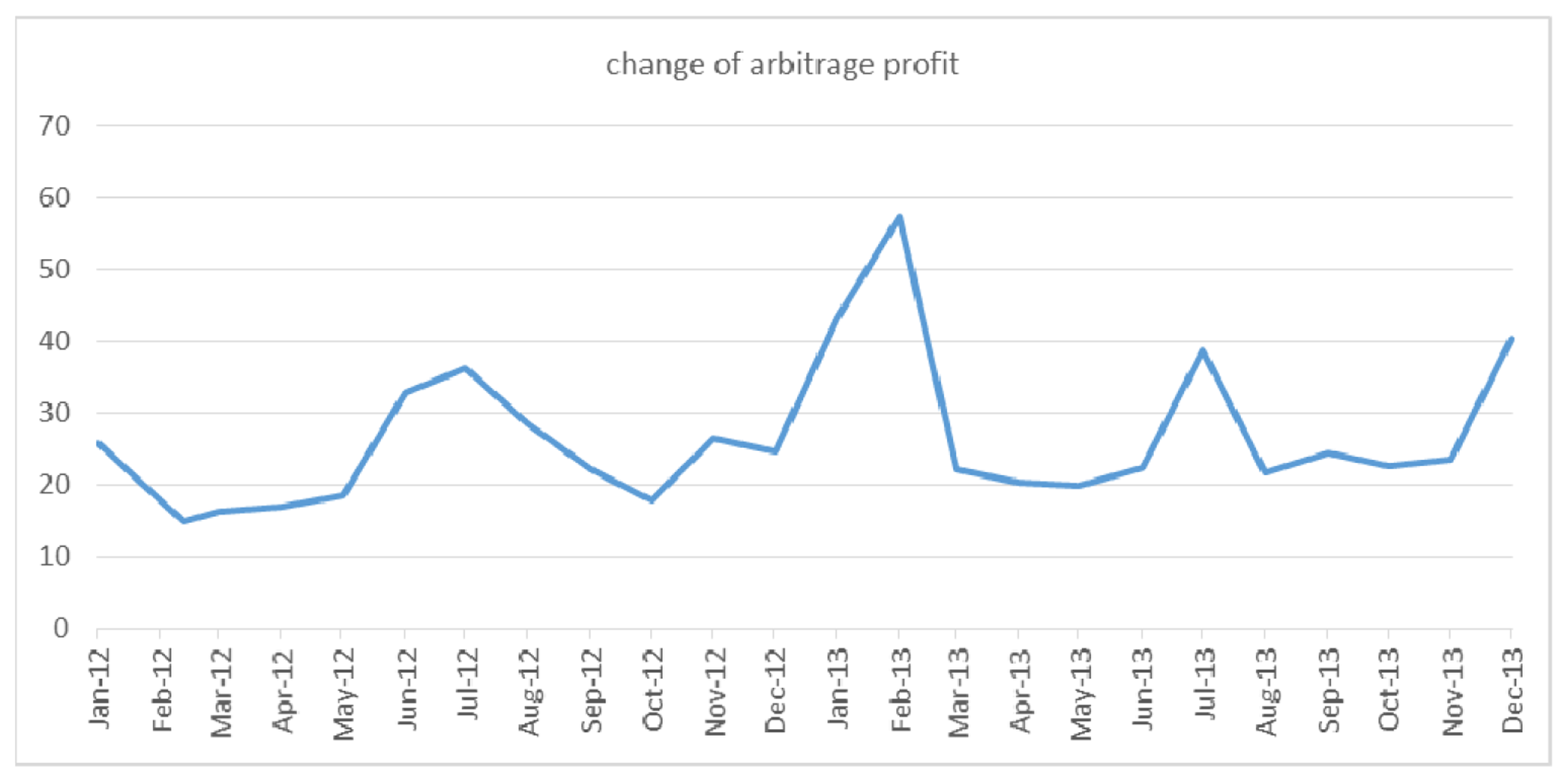
To estimate the volatility of the arbitrage profit function, first, we derive a minimum value and a maximum value among the averages of four consecutive hours during a day. Note that, in the latter section, we also estimate volatilities for the case of three and five consecutive hour operation policies. Then, for the time period having the minimum prices, ESS will charge electricity to a capacity level and, for the time having the maximum prices, it will discharge at a rate of loss, η. The difference between two time periods can be calculated. Then, we calculate averages of those differences monthly. The value of the difference is shown in the following figure and we can recognize the data is very volatile over time.

From the data set for an arbitrage profit function, it is necessary to estimate volatility. For the parameter estimation, we applied the continuous method corresponding to a continuous rate of return, which can be computed as follows:

$$R{e}_i=ln\left(\frac{P_i}{P_{i-1}}\right)$$

(18)

For the transformed data, the log-returns of arbitrage profits, we compute the average value of the returns, $\overline{\mathit{\text{Re}}}=\frac{1}{n}{\text{∑}}_{\text{i}=1}^n{\mathit{\text{Re}}}_i$, where n is the number of returns. The standard deviation is used to estimate volatility and it is annualized as follows:

$$\sigma =\frac{1}{\sqrt{dt}}\sqrt{\frac{1}{n-1}\text{∑}_{i=1}^n{(R{e}_i-\overline{Re})}^2}$$

(19)

Then, basic statistics for computed log-return data are given in the following table.

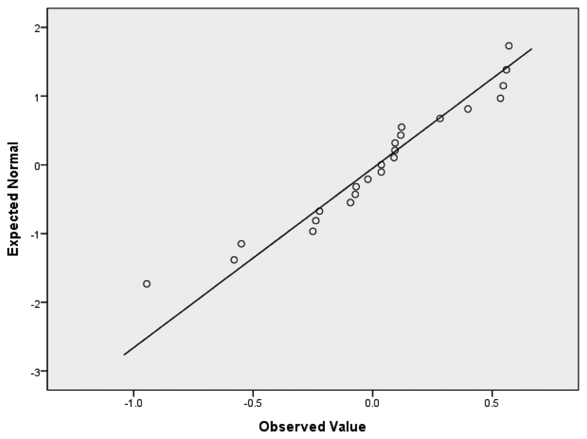
The property of geometric Brownian motion is that logarithm of return follows a normal distribution. Therefore, we checked the normality of our data using the SPSS software. As shown in

Table 2. Test of normality for log-return.

Tests of Normality
Variable	Kolmogorov-Smirnov a			Shapiro-Wilk
	Statistic	df	Sig.	Statistic	df	Sig.
Arbitrage	0.134	23	0.200 *	0.941	23	0.188

* This is a lower bound of the true significance;^a Lilliefors Significance Correction.

, the data tested by the Komogorov-Smirnov and Shapiro-Wilk methods shows the data set follows normal distribution at the significant level of 0.05. Also, we could check how the data are scattered along with the mean from Figure 2.

4.2. The Impact of Uncertainty and Mean Drift

The impact of uncertainty could be important in investment decisions as described in [2,7]. Therefore, in this section, we investigate the impact of uncertainty which is represented by volatility. Also, the effects of mean-drift and ESS cost as an investment sunk cost on optimal threshold are studied. To run the simulation, we use the parameters in the following table.

Before discuss the impact of uncertainty, we want to figure out the relationship between uncertainty and the properties of the ESS. From the data set and methods described in the previous subsection, the volatilities for different efficiency levels can be calculated. The efficiency level is related to the technical specification of the ESS. For example, depth of discharge may differ for different ESS manufacturers. The Sandia Lab report shows that the depth of discharge ranges from 0.8 to 1 and the round trip efficiency varies from 0.8 to 0.94, depending on ESS supplier [17]. Due to this technical limitation of ESSs, it cannot fully discharge the charged electricity. For example, it can charge only 80% of charged and stored electricity. However, the level of efficiency becomes higher in accordance with ESS technology development and the efficiency could reach to the level of near 1 in the future. For this reason, we conduct our experiments and do sensitivity analysis, while using the efficiency level from 0.8 to maximally 1. Herein, note that efficiency level of 1 is used as a reference of maximum efficiency level and it is very challenging to technically achieve the level.

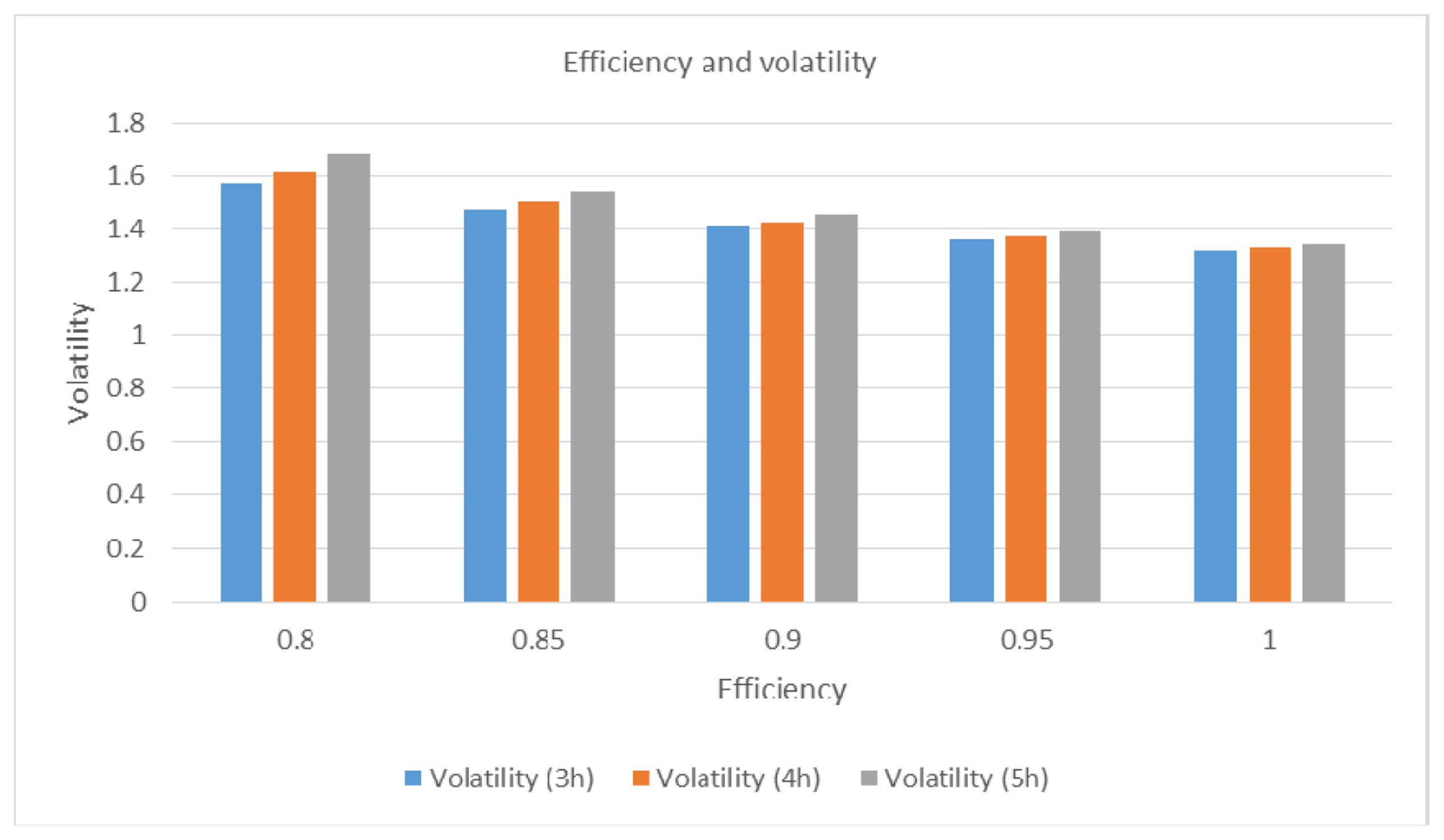
Therefore, we investigated how the efficiency affects uncertainty level of arbitrage profit. As shown in

Table 4. Efficiency, operation duration and volatility.

Efficiency	1	0.95	0.9	0.85	0.8
Volatility (3 h)	1.320071	1.358877	1.408915	1.475845	1.569939
Volatility (4 h)	1.32695	1.370017	1.426318	1.503024	1.613711
Volatility (5 h)	1.340524	1.389001	1.453371	1.542958	1.676337

and Figure 3, as the efficiency level becomes higher, volatility decreases. Also, the uncertainty level might be related to operation duration. In this experiment, we have computed the data into three cases, 3 h, 4 h and 5 h operations. In other words, we assume that a firm charges for 3, 4 and 5 h and then discharges electricity for the same amount of time. For those three scenarios, when we compare volatilities, we found that the volatility increases as operation duration becomes longer. Conclusively, our results show that, as ESS gets more efficient and operation duration are shorter, volatility becomes lower, which implies that uncertainty of profits from arbitrage trade is reduced.

Thus far, we have investigated the relationship between uncertainty and characteristics of ESSs such as efficiency and operation policy. From now, we analyze the impact of uncertainty on the optimal investment time or threshold.

Proposition 1. (Optimal investment time and Uncertainty). The threshold for an ESS investment is increasing in increasing volatility. Simply, more uncertain arbitrage profit makes it more difficult for the investor to invest in an ESS. Besides, this implies that if the efficiency of an ESS increases, the launch of the ESS will be expedited even for the same power capacity.

Since the optimal investment time is given in the form of $P^{*}=\frac{{\beta }_1(r-\mu )}{({\beta }_1-1)(1-e^{-(r-\mu )D})}I$, we examine the relationship between volatility (σ) and the threshold (P*). To verify this property described in Proposition 1, we take derivative of P* with respect to volatility (σ). This leads to:

$$\frac{\partial }{\partial \sigma }{P}^{*}=\frac{\partial }{\partial {\beta }_1}{P}^{*}\frac{\partial {\beta }_1}{\partial \sigma }=\frac{\left(r-\mu \right)}{(1-e^{-\left(r-\mu \right)D})Q}I\frac{\partial {\beta }_1}{\partial \sigma }\frac{\partial }{\partial {\beta }_1}\left(\frac{{\beta }_1}{{\beta }_1-1}\right)=-\frac{\left(r-\mu \right)}{(1-e^{-\left(r-\mu \right)D})Q}I{\left(\frac{1}{{\beta }_1-1}\right)}^2\frac{\partial {\beta }_1}{\partial \sigma }$$

(20)

This result is dependent of $\frac{\partial {\beta }_1}{\partial \sigma }$ , so let us check the sign as follows. First, let $U\left({\beta }_i\right)=\frac{1}{2}{\sigma }^2\beta \left(\beta -1\right)+\mu \beta -r$ from Equation (12) and take a derivative:

$$\frac{\partial U}{\partial \beta }\frac{\partial {\beta }_i}{\partial \sigma }+\frac{\partial U}{\partial \sigma }=0,\text{for}i=1,2$$

(21)

Herein, derivatives are evaluated at β₁ and β₂. And we know $\frac{\partial U}{\partial \beta }>0$ at β₁ and $\frac{\partial U}{\partial \beta }<0$ at β₂ since U is quadratic, β₁ > 1 and β₂ > 0. Moreover, $\frac{\partial U}{\partial \sigma }=\sigma {\beta }_i({\beta }_i-1)>0\text{fori}=1,2$. From these inequality conditions, we have:

$$\frac{\partial {\beta }_1}{\partial \sigma }<0\text{and}\frac{\partial {\beta }_2}{\partial \sigma }>0$$

(22)

Besides, since $\frac{(r-\mu )}{(1-e^{-\left(r-\mu \right)D})Q}I>0$, the derivative is:

$$\frac{\partial }{\partial \sigma }{P}^{*}==-\frac{\left(r-\mu \right)}{(1-e^{-\left(r-\mu \right)D})Q}I{\left(\frac{1}{{\beta }_1-1}\right)}^2\frac{\partial {\beta }_1}{\partial \sigma }>0$$

(23)

This result implies that the optimal time to invest in an ESS increases in increasing volatility as explained in Proposition 1. The more volatile the arbitrage profit becomes, the higher the threshold that is expected, which causes the delay of investment. For this result, we have run simulations for different volatilities, from 0.2 to 2.2, and the result is shown in Figure 4. The threshold increases drastically, when volatility increases. Furthermore, when we consider the relationship between uncertainty and efficiency of ESS, we can notice that since uncertainty becomes smaller as efficiency increases, higher efficiency might enables earlier investment.

Next, let us discuss the impact of mean drift and ESS cost on investment time.

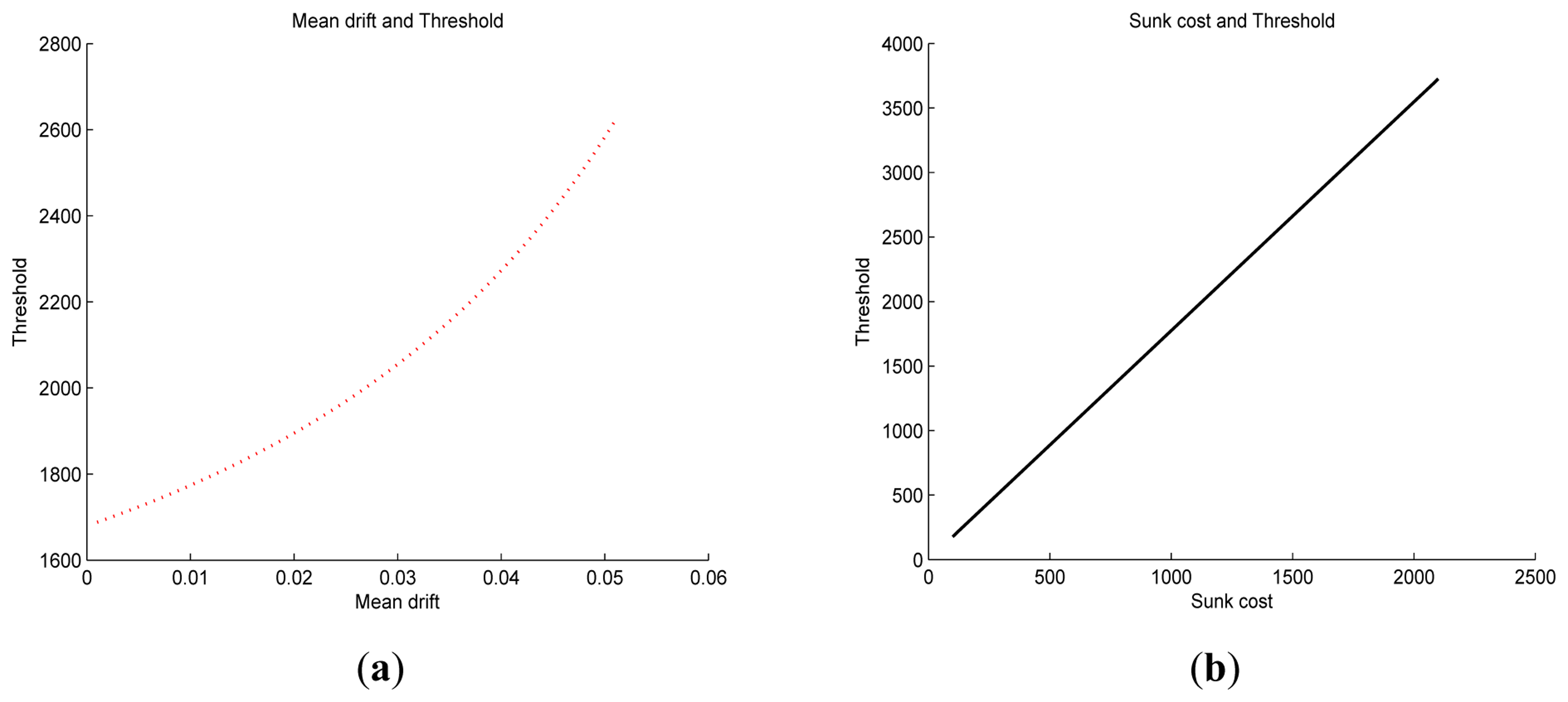
Proposition 2. (Optimal investment time, mean drift and ESS cost). The threshold for an ESS investment is increasing in increasing mean drift and ESS cost. This implies that when a higher rate of return is expected in the future, the investor is more likely to wait. Also, if the ESS cost is higher, the investor needs to wait longer.

First, we try to verify the impact of mean drift:

$$\frac{\partial {\beta }_1}{\partial \mu }=-\frac{2}{{\sigma }^2}+\frac{2\left(1-\frac{2\mu }{{\sigma }^2}\right)}{{\sigma }^2\sqrt{{\left(1-\frac{2\mu }{{\sigma }^2}\right)}^2+\frac{8r}{{\sigma }^2}}}=\frac{{\beta }_1}{{\sigma }^2\sqrt{{\left(1-\frac{2\mu }{{\sigma }^2}\right)}^2+\frac{8r}{{\sigma }^2}}}<0$$

(24)

$$\frac{\partial }{\partial \mu }{P}^{*}=\frac{\partial }{\partial {\beta }_1}{P}^{*}\frac{\partial {\beta }_1}{\partial \mu }=\frac{\left(r-\mu \right)}{(1-e^{-\left(r-\mu \right)D})Q}I\frac{\partial {\beta }_1}{\partial \mu }\frac{\partial }{\partial {\beta }_1}\left(\frac{{\beta }_1}{{\beta }_1-1}\right)=-\frac{\left(r-\mu \right)}{(1-e^{-\left(r-\mu \right)D})Q}I{\left(\frac{1}{{\beta }_1-1}\right)}^2\frac{\partial {\beta }_1}{\partial \mu }>0$$

(25)

Besides, the derivative with respect to investment sunk cost (I) is simply derived as follows:

$$\frac{\partial }{\partial I}{P}^{*}=\frac{(r-\mu )}{(1-e^{-\left(r-\mu \right)D})Q}\left(\frac{{\beta }_1}{{\beta }_1-1}\right)>0$$

(26)

For two derivations, we can obtain the results described in Proposition 2. Interestingly, we found that if arbitrage profits increase, it is more beneficial to wait for a while. This result might seem counterintuitive. However, it could be interpreted that because the higher expected profits during the lifetime of a ESS could be made if we wait as longer as possible, an investor needs to wait. However, in practice, the investor could invest in ESSs repeatedly after obsolescence, which can change this result. For the second result in Proposition 2, it is quite intuitive that increased ESS cost will make the investor wait longer. From simulation, we have Figure 5 describing Proposition 2.

4.3. Decision Making by Real Option and Net Present Value (NPV) and Comparison

As mentioned in many studies, the impact of uncertainty on the investment decision is not ignorable and is sometimes quite critical. This is also reported in ESS literature as well. Reference [2] found that the probabilities of the futures can influence the optimal ESS sizing problem and emphasized the importance of addressing uncertainty in decision making. In addition to uncertainty, we considered a firm's option to wait. Therefore, in this section we examine how results differ by comparing a classical method to our proposed model.

The traditional net present value (NPV) method which has been widely used can also provide a way to evaluate an ESS investment. However, the NPV cannot capture a value of decision flexibility, i.e., when to invest in an ESS. The NPV method only determines whether or not to invest in ESSs. Thus, in this subsection, we examine what happens if we do not consider the decision flexibility by comparing the strategies by NPV and a real option theory (ROT). By comparing profit cash flows before and after introducing ESS from the NPV perspective, we can derive the optimal threshold (P*_NPV) for ESS investment as follows:

$$V_{\mathit{\text{NPV}}}\left(P\right)=\{\begin{array}{cc}0& \mathit{if}P<P_{\mathit{\text{NPV}}}^{*}\\ QP\frac{1-e^{-\left(r-\mu \right)D}}{r-\mu }-I& \mathit{if}P\ge P_{\mathit{\text{NPV}}}^{*}\end{array}$$

(27)

From the value function (27), an investment threshold by NPV is derived from:

$$QP\frac{1-e^{-\left(r-\mu \right)D}}{r-\mu }-I=0$$

(28)

Therefore, we have:

$${P^{*}}_{\mathit{\text{NPV}}}=\frac{(r-\mu )}{Q(1-e^{-\left(r-\mu \right)D})}I$$

(29)

Proposition 3. ESS investment feasible region determined by NPV ( $P_{\mathit{\text{NPV}}}^{\mathit{\text{fea}}}$) is always larger than that by ROT ( $P_{RO}^{\mathit{\text{fea}}}$). This implies that an investor should wait longer than expected.

$$P_{RO}^{\mathit{\text{fea}}}=\{P|P\ge P_{RO}^{*}\}\subset P_{\mathit{\text{NPV}}}^{\mathit{\text{fea}}}=\{P|P\ge P_{\mathit{\text{NPV}}}^{*}\}$$

The previous results gives us:

$${P^{*}}_{\mathit{\text{NPV}}}=\frac{(r-\mu )}{Q(1-e^{-\left(r-\mu \right)D})}I$$

(30)

$${P^{*}}_{RO}=P^{*}=\frac{{\beta }_1(r-\mu )}{Q({\beta }_1-1)(1-e^{-\left(r-\mu \right)D})}I$$

(31)

$$\frac{{P^{*}}_{RO}}{{P^{*}}_{\mathit{\text{NPV}}}}=\frac{{\beta }_1}{\left({\beta }_1-1\right)}$$

(32)

since $\frac{{\beta }_1}{\left({\beta }_1-1\right)}>1$, P*_RO> P*_NPV.

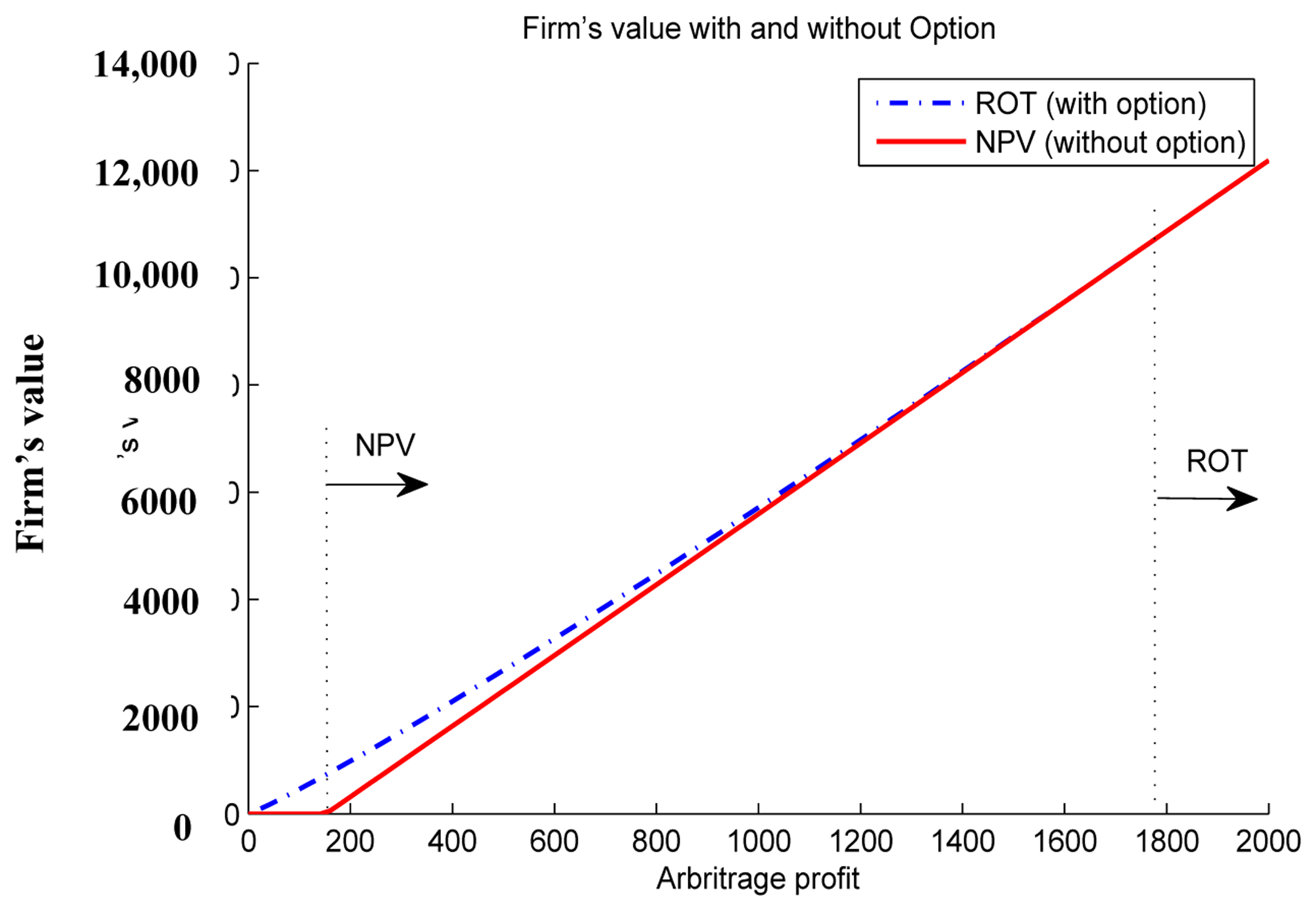
Proposition 3 implies that the traditional method is always less strict than the real option theory. Through simulations, we evaluate a firm's values using NPV and ROT, and derive the corresponding optimal thresholds. As shown in Figure 6, the firm's value by ROT is higher than its value by NPV, and the threshold by NPV (P*_NPV = 151.6) is smaller than the threshold by ROT (P*_RO = 1773.8). Also, the feasible region where a firm can invest is on the right-hand side of the dotted lines. This result implies that, for example, if profit cash flow is 1000, then the ESS investment decision is appropriate from the NPV perspective, while it is inappropriate from the ROT perspective. For this particular range of arbitrage profit, the NPV suggests ESS introduction, but the ROT recommends a firm to wait for a while and to invest later. Also, we can find that the threshold by ROT is 11.8 times the threshold by NPV, which indicates the importance of volatility and optionality. In other words, consideration of option under uncertainty gives a significantly different decision.

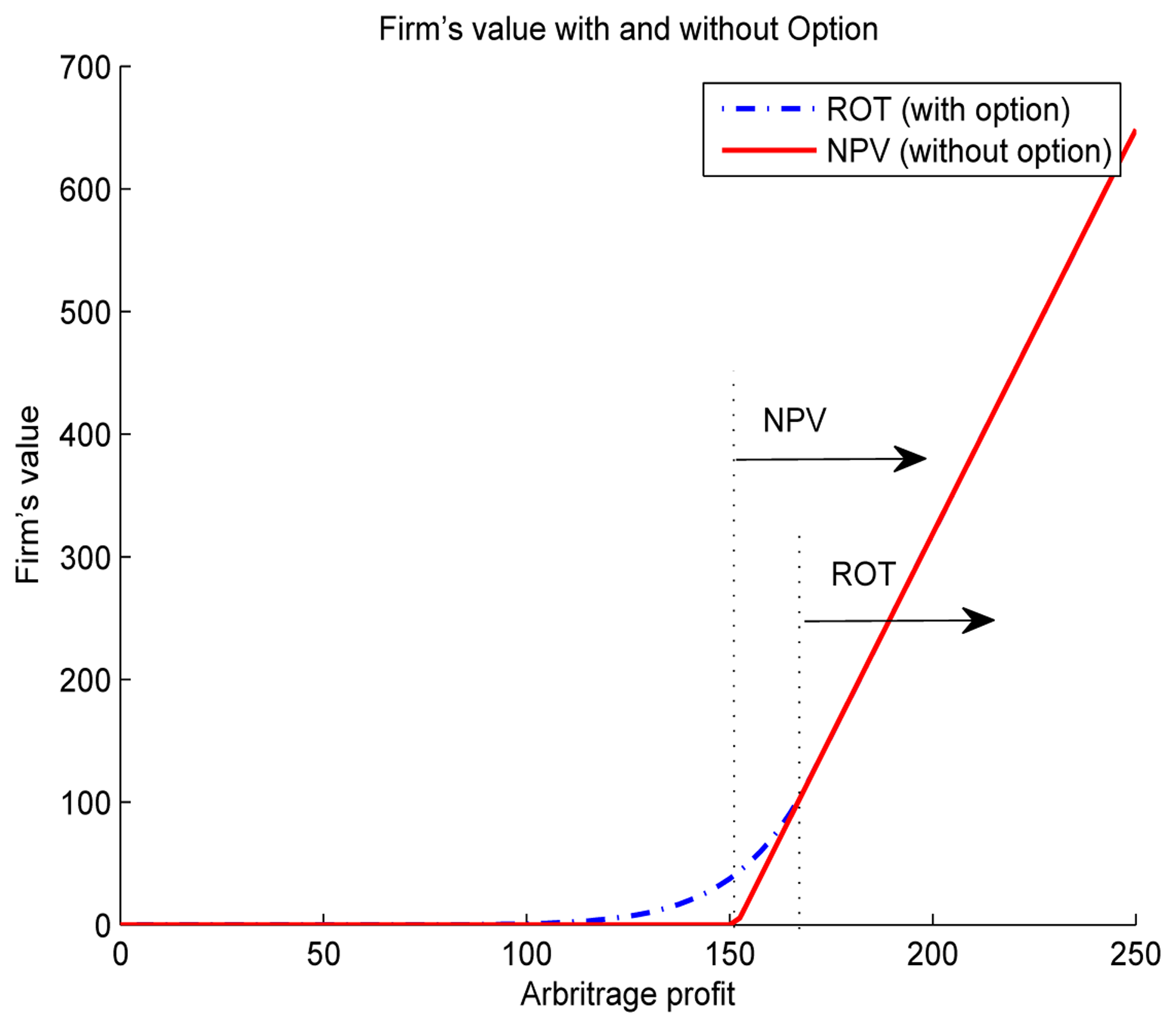
Moreover, depending on the environment, the level of uncertainty may change and the decision might differ. Therefore, we investigate the change of investment thresholds and the difference. When volatility is decreased to 0.013, the threshold becomes 169.9 and 151.7. The threshold by ROT is 1.12 times the threshold by NPV, as shown in Figure 7. When we compare results for small and large volatility, the difference between two thresholds significantly decreases as volatility is reduced. However, for both cases, value functions and thresholds given by ROT are always larger than the value functions and thresholds by NPV as explained in Proposition 3.

In addition, let us discuss how much the firm's value changes, as we do not consider the firm's option to wait.

Table 5. Percentage of investment value uncaptured by NPV.

μ	σ
	0.2			0.6			1.0
	I			I			I
	500	1000	1500	500	1000	1500	500	1000	1500
0.01	0.00	16.48	0.00	4.27	109.48	30.00	18.92	174.65	60.87
0.015	0.00	16.38	0.00	4.54	102.45	29.56	18.86	162.33	59.01
0.02	0.00	16.62	0.00	4.86	96.56	29.25	18.86	151.74	57.35
0.025	0.00	17.16	0.02	5.23	91.63	29.09	18.91	142.58	55.89
0.03	0.00	17.99	0.18	5.66	87.51	29.07	19.01	134.63	54.61
0.035	0.00	19.12	0.56	6.15	84.10	29.20	19.17	127.70	53.50

shows the percentage of the option value that is not captured by the NPV approach, compared to the ROT. Experiments were conducted for three different factors like volatility, mean drift and ESS cost. Uncaptured values that are lost by applying the NPV approach are from 0 to 174.65%. This result implies that a firm might underestimate an ESS investment.

5. Conclusions and Further Study

This paper proposes a model to determine the optimal investment time for energy storage systems in application of price arbitrage trade under conditions of uncertainty over future profits. In previous literature discussing ESS investment evaluation, two aspects, an option of a firm and uncertainty of profits, have not been paid attention. Despite the many benefits, if the investment is not profitable at a certain point in time, the utility firm would not invest and wait until the cost of the ESS would decrease or profits from an ESS would increase. Also, the profits obtained from operating an ESS and trading electricity are uncertain. Therefore, we suggest a real option model considering these two important factors to determine when the optimal investment time is. Then, we analyze the investment with respect to several characteristics of uncertainty. Our model provides an optimal threshold to invest in an ESS so that a firm can start to invest as soon as the profit level has reached the optimal threshold. Otherwise, the firm needs to wait until it reaches to the threshold.

Our results about the optimal time to invest show that as profits obtained from arbitrage trade become more uncertain, an investor needs to wait longer. Also, improvement of efficiency in the ESS can reduce the uncertainty of arbitrage profit and, consequently, the reduced uncertainty enables earlier ESS investment, even for the same power capacity. Besides, when an expected rate of profits and ESS costs are higher, an investor needs to wait longer. Finally, our analyses show that a classical net present value method and a real option method, which is proposed in this paper, give significantly different results. The comparison of a real option approach and a net present value method shows that the net present value method underestimates the value of ESS investment and suggests an investment time 1.12 times to 11.8 times earlier than the optimal time. It is also found that the uncaptured value by a net present value method is up to 174.65 percent, which is too large to be ignored.

As an extension of this research, the multi-purpose operation of ESSs can be considered. As described in [16,17], ESSs have 17 application areas such as electric supply, ancillary service, grid system, end use, renewables integration, etc. However, for example, a portion of ESS capacity can be used for arbitrage trade and the rest can be applied to ancillary service. Or, for different time periods, different services can be provided depending on profitability over time. For our model to be more realistic and practical, the assumption of Geometric Brownian motion can be substituted by more sophisticated models, such as mean reverting process model and autoregressive conditional heteroskedasticity (ARCH) model. Moreover, in practice, a firm can invest in ESS repeatedly after obsolescence, while our model assumes one time investment. Because repeated investment maximizes profit and the future cost of ESS is expected to decrease, the results could be different. Also, uncertain cost can be another extension of this research. In the case of Li-ion batteries, the cost is decreasing and is expected to reach to half of current cost within several years. Taking the cost uncertainty into account may lead to different investment times.

References

- Bradbury, K.; Pratson, L.; Patiño-Echeverri, D. Economic viability of energy storage systems based on price arbitrage potential in real-time U.S. electricity markets. Appl. Energy 2014, 114, 512–519. [Google Scholar]
- Carpinelli, G.; di Fazio, A.R.; Khormali, S.; Mottola, F. Optimal sizing of battery storage systems for industrial applications when uncertainties exist. Energies 2014, 7, 130–149. [Google Scholar]
- Walawalkar, R.; Apt, J.; Mancini, R. Economics of electric energy storage for energy arbitrage and regulation in New York. Energy Policy 2007, 35, 2558–2568. [Google Scholar]
- Electric Power Research Institute (EPRI). Cost-Effectiveness of Energy Storage in California; EPRI: Palo Alto, CA, USA, 2013. [Google Scholar]
- Denholm, P.; Jorgenson, J.; Hummon, M.; Jenkin, T.; Palchak, D.; Kirby, B.; Ma, O.; O'Malley, M. The Value of Energy Storage for Grid Applications; Technical Report NREL/TP-6A20-58465; National Renewable Energy Laboratory (NREL): Golden, CO, USA, 2013. [Google Scholar]
- Rudolf, V.; Papastergiou, K.D. Financial analysis of utility scale photovoltaic plants with battery energy storage. Energy Policy 2013, 63, 139–146. [Google Scholar]
- Dixit, A.K.; Pindyck, R.S. Investment under Uncertainty; Princeton University Press: Princeton, NJ, USA, 1994. [Google Scholar]
- Pindyck, R.S. Sunk Costs and Real Options in Antitrust; National Bureau of Economic Research: Cambridge, MA, USA, 2005. [Google Scholar]
- Kogut, B.; Kulatilaka, N. Operating flexibility, global manufacturing, and the option value of a multinational network. Manag. Sci. 1994, 40, 123–139. [Google Scholar]
- Grenadier, S.R.; Weiss, A.M. Investment in technological innovations: An option pricing approach. J. Financ. Econ. 1997, 44, 397–416. [Google Scholar]
- Wu, G.; Zhou, H.; Pan, W.; Hou, Y. Life cycle management method for smart grid asset with real option theory. Proceedings of the 2012 3rd IEEE PES International Conference and Exhibition on Innovative Smart Grid Technologies (ISGT Europe), Berlin, Germany, 14–17 October 2012; pp. 1–6.
- Cartea, Á; González-Pedraz, C. How much should we pay for interconnecting electricity markets? A real options approach. Energy Econ. 2012, 34, 14–30. [Google Scholar]
- Muche, T. A real option-based simulation model to evaluate investments in pump storage plants. Energy Policy 2009, 37, 4851–4862. [Google Scholar]
- Kumbaroğlu, G.; Madlener, R.; Demirel, M. A real options evaluation model for the diffusion prospects of new renewable power generation technologies. Energy Econ. 2008, 30, 1882–1908. [Google Scholar]
- Marreco, J.D.M.; Carpio, L.G.T. Flexibility valuation in the Brazilian power system: A real options approach. Energy Policy 2006, 34, 3749–3756. [Google Scholar]
- Eyer, J.; Corey, G. Energy Storage for the Electricity Grid: Benefits and Market Potential Assessment Guide; Report SAND2010-0815; Sandia National Laboratories: Albuquerque, NM, USA, 2010. [Google Scholar]
- Akhil, A.A.; Huff, G.; Currier, A.B.; Kaun, B.C.; Rastler, D.M.; Chen, S.B.; Cotter, A.L.; Bradshaw, D.T.; Gauntlett, W.D. DOE/EPRI 2013 Electricity Storage Handbook in Collaboration with NRECA; SANDIA Report SAND2013-5131; Sandia National Laboratories: Albuquerque, NM, USA, 2013. [Google Scholar]
- Wade, N.S.; Taylor, P.; Lang, P.; Jones, P. Evaluating the benefits of an electrical energy storage system in a future smart grid. Energy Policy 2010, 38, 7180–7188. [Google Scholar]
- Sioshansi, R.; Denholm, P.; Jenkin, T.; Weiss, J. Estimating the value of electricity storage in PJM: Arbitrage and some welfare effects. Energy Econ. 2009, 31, 269–277. [Google Scholar]
- Yu, W.; Liu, D.; Huang, Y. Operation optimization based on the power supply and storage capacity of an active distribution network. Energies 2013, 6, 6423–6438. [Google Scholar]
- Abadie, L.M. Valuation of long-term investments in energy assets under uncertainty. Energies 2009, 2, 738–768. [Google Scholar]
- Brennan, M.J.; Schwartz, E.S. Evaluating natural resource investments. J. Bus. 1985, 58, 135–157. [Google Scholar]
- McDonald, R.; Siegel, D. The value of waiting to invest. Q. J. Econ. 1986, 101, 707–728. [Google Scholar]
- Dixit, A. Entry and exit decisions under uncertainty. J. Polit. Econ. 1989, 97, 620–638. [Google Scholar]
- Schwartz, E.S.; Zozaya-Gorostiza, C. Investment under uncertainty in information technology: Acquisition and development projects. Manag. Sci. 2003, 49, 57–70. [Google Scholar]
- Pindyck, R.S. Irreversibility,uncertainty, and investment. J. Econ. Lit. 1991, XXIX, 1110–1148. [Google Scholar]
- Luehrman, T.A. Investment opportunities as real options: Getting started on the numbers. Harv. Bus. Rev. 1998, 76, 51–67. [Google Scholar]
- Zhu, K.; Weyant, J.P. Strategic decisions of new technology adoption under asymmetric information: A game-theoretic model. Decis. Sci. 2003, 34, 643–675. [Google Scholar]
- Huchzermeier, A.; Loch, C.H. Project management under risk: Using the real options approach to evaluate flexibility in R&D. Manag. Sci. 2001, 47, 85–101. [Google Scholar]
- Tang, S.; Yu, C.; Wang, X.; Guo, X.; Si, X. Remaining useful life prediction of lithium-ion batteries based on the wiener process with measurement error. Energies 2014, 7, 520–547. [Google Scholar]
- Benaroch, M. Managing information technology investment risk: A real options perspective. J. Manag. Inf. Syst. 2002, 19, 43–84. [Google Scholar]
- Wilmott, P. The Mathematics of Financial Derivatives: A Student Introduction; Cambridge University Press: Cambridge, UK, 1995. [Google Scholar]