Exponential Smoothing Approaches for Prediction in Real-Time Electricity Markets

Abstract

The optimal design of offering strategies for wind power producers is commonly based on unconditional (and, hence, constant) expectation values for prices in real-time markets, directly defining their loss function in a stochastic optimization framework. This is why it may certainly be advantageous to account for the seasonal and dynamic behavior of such prices, hence translating to time-varying loss functions. With that objective in mind, forecasting approaches relying on simple models that accommodate the seasonal and dynamic nature of real-time prices are derived and analyzed. These are all based on the well-known Holt–Winters model with a daily seasonal cycle, either in its conventional form or conditioned upon exogenous variables, such as: (i) day-ahead price; (ii) system load; and (iii) wind power penetration. The superiority of the proposed approach over a number of common benchmarks is subsequently demonstrated through an empirical investigation for the Nord Pool, mimicking practical forecasting for a three-year period over 2008–2011.

1. Introduction

In parallel with the rapid growth in electricity generation by renewable energy sources, producers are increasingly urged to sell their generation though the market. This has triggered the interest of both researchers and practitioners in proposing optimal bidding strategies for renewable energy producers as balance responsible parties (BRPs) in deregulated electricity markets. Especially, wind power appears to have a leading role among recently emerging renewable energy sources. The wind power producer's point of view will also be considered here for the sake of an example. Other market participants may be interested in the forecasting of regulation market quantities for optimization of their market participation strategies. Wind power production is a stochastic process with limited predictability on a day-ahead basis. Accordingly, the offering strategies of wind power producers are derived in a stochastic optimization framework. The resulting optimization problems aim at minimizing the expected costs induced by their (involuntary) participation in the real-time imbalance market (also referred to as regulation market), potentially also accounting for risk aversion [1–8].

The unit regulation costs (per MWh of imbalance) in the real-time market are dynamic and asymmetric [9]. As shown by [10] in the general case and by [1] for wind power specifically, this makes common bidding procedures solely based on the expected generation for every lead time sub-optimal. Instead, the bid maximizing expected revenues is found to be a particular quantile of predictive production densities. The nominal level of this quantile is a direct function of expected unit regulation costs in the real-time market, also referred to as imbalance penalties. Despite their obvious impact on the performance of trading strategies, these quantities are often assumed deterministic and known [2] or model-based on long-term averages [3,6,7], hence disregarding the short-term dynamics of the real-time market. Under similar assumptions, [11] conclude that gaming in general cannot be profitable. Recently though, [4], [5] and [8] have taken into account short-term variations in the penalties with considerable benefits. The drawback of the approach of [5] and [8] is that their models cannot accommodate negative prices, even though they are a reality of many electricity markets. Furthermore, information that was not available before the market gate closure is used. In contrast, the results of [4] are obtained using the forecasting methodology described in the present paper, hence yielding optimal bids based entirely on predictions from readily available information prior to gate closure.

The objective of this paper is to rigorously model and predict imbalance penalties, at the lead times of interest, when trading wind power in a day-ahead market, in an exponential smoothing framework. The very nature of regulation markets makes that real-time electricity price modeling ought to differ substantially from conventional time series modeling approaches. Excessive volatility and skewness aside, anti-gaming policies have in many cases caused these prices to exhibit unique dynamic features. Firstly, the widely adopted dual pricing scheme for regulating power (which implies different pricing for producers in surplus and deficit) induces a regime-switching behavior in the prices, driven by the net balance of the system. Additionally, some markets have real-time prices that are bounded by the day-ahead price (e.g., the Danish and the Spanish ones) or capped in another manner (e.g., the Pennsylvania-New Jersey-Maryland—PJM, and the New England markets in the USA) to discourage gaming even further. This feature magnifies the state dependency of the prices, since they either share characteristics with the day-ahead prices or have their own unique dynamics. Furthermore, this policy arguably inflates the volatility in the real-time market through reduced supply.

Conditioning models for the real-time prices on the net balance of the whole system is paramount for capturing relevant price dynamics. This, in turn, makes popular time series models, like the seasonal Auto-Regressive Moving Average (ARMA) model used in [5], inadequate, since this type of model does not account for this regime-switching behavior. Olsson and Söder [12] introduced a Markov-switching seasonal ARIMA model with time-inhomogeneous transition probabilities for addressing this issue, though with the following pitfalls. Firstly, the transition probabilities are time-invariant, hence ignoring the short-term variations in state probabilities, while such variations are shown to be substantial in this paper. Secondly, the lack of auto-correlation between day-ahead lags causes the time-inhomogeneous transition probabilities to converge to the homogeneous ones rather quickly, and for lead times shorter than those required for bidding into a day-ahead market. Put differently, the transition probability matrices for lead times required for the day-ahead trading of wind power contain only the empirical steady-state distribution during the period on which the estimation is based.

The idea behind the prediction approach introduced here is to take advantage of the formulation of imbalance costs as the product of two variables: (i) a categorical one representing the sign of the net system balance; and (ii) a penalty part describing the magnitude of imbalance penalties when active. Combining predictions for these two variables by applying the law of total expectation then yields the expected imbalance costs. Both variables are modeled using Holt–Winters models [13] with a daily seasonal cycle, either in its conventional form or conditioned by exogenous variables. The proposed approach is to be evaluated against a climatology benchmark, for each individual variable and for the final expected imbalance penalties.

The remainder of the paper is structured as follows: Section 2 gives an overview of the empirical context of the paper and describes the data used for the analysis. Afterwards, the necessary definitions and data analysis are presented in Section 3. The models and parameter estimation procedures are given in Section 4, followed by the results of our empirical investigation in Section 5. Finally, concluding remarks are gathered in Section 6.

2. Specific Characteristics and Data for Nord Pool

Day-ahead electricity markets are the result of a general movement around the world towards deregulation in the electricity industry over the past two decades. Although the actual implementation varies between countries and regions, the basic functionalities remain similar among those who have adopted these policies. Even though emphasis is placed here on the Nord Pool electricity market in Scandinavia, the proposed models and forecasting methodologies may certainly be appropriate for other electricity markets (with some variations in forecast performance). After first presenting some of the specifics of the Nord Pool, the dataset available for our modeling and forecasting study is described in detail.

2.1. Nord Pool and the Danish Electricity Market

The Danish electricity market is a part of the Nord Pool market, which is the world's first multinational electricity market. It was founded by Statnett SF and Svenska Kraftnät (the Norwegian and Swedish Transmission System Operators (TSOs), respectively) in 1996. Since then, it has been gradually expanded to encompass Denmark, Finland and Estonia, as well. In 2002, physical exchange activities were transferred to a separate company, Nord Pool Spot ASA, which operates the markets. It is jointly owned by Statnett SF, Svenska Kraftnät (30% each), Energinet.dk and Fingrid Oy (20% each). Nord Pool's market share is one of the highest in the world with 72% of the total Nordic consumption traded on its markets in 2009 [14]. In 2010 and 2011, the market share rose to 74% and 75%, respectively [15,16].

The market region is divided into 10 price areas, bordered by bottlenecks in the transmission grid and with internal transmission capacity practically infinite. Denmark comprises two of these areas, one on either side of the Storebælt channel.

Nord Pool runs two different markets for the physical exchange of electricity, Elspot and Elbas. Elspot is a day-ahead market with gate closure at noon on the day before delivery. Here, producers and retailers bid for the sale and purchase of electricity in hourly intervals. Once the bids are collected, a system price is determined as the intersection between the aggregated supply and demand curves. The system price is the price at which the physical exchange is settled during hours where transmission across the grid bottlenecks does not reach capacity. Besides, the system price serves as a reference price for almost all financial derivatives linked to Nord Pool. In case the desired transmission across price area borders reaches its capacity, multiple area prices are defined. An area price is determined by the same procedure as the system price, though only considering the bids from the particular area, and the full usage of the connections to the surrounding areas as price-independent bids. Elbas is opened for trading once Elspot prices have been published and has gate closure one hour prior to delivery. Elbas is a bid-ask market where bids for either the purchase or sale of electricity are placed. The bids are prioritized according to price and submission time. They are settled at the bid price. The acceptance of a bid across price areas is subject to capacity availability. Almost the entire exchange takes place on Elspot, which is responsible for more than 99% of the total exchanged volume each year. A more detailed description of the market environment and price settlement is provided in [17].

In addition, the national TSOs each run a real-time market in their countries for balancing the transmission grid. Markets for supplier imbalances and retailer imbalances are run separately and with different pricing schemes. For the retailers, a single price is defined at which those short of their contracted volume buy the surplus of those having overestimated their consumption at the time. In contrast, two prices are defined on the suppliers' market. The producers short of their contracts buy their deficits at the up-regulation price, while those overproducing sell their surplus at the down-regulation price. The regulation prices are bounded by the Elspot prices, so that the up-regulation price can never deceed it and the down-regulation price can never exceed it. Furthermore, imbalances that negate the total system imbalance are not penalized. This implies that at any given time, either the up-regulation or the down-regulation price is equal to the spot price.

2.2. Available Data for the Study

The data for the empirical investigation covers the period from November, 2008, to December, 2011. The dataset includes hourly spot and regulation prices for the Western Danish price area of Elspot (DK-1) along with predicted system load, wind power production and spot prices for the same area. All forecasts are issued before noon on the day before delivery. They also have an hourly temporal resolution. The observed prices and the load forecasts are publicly available on the website of Nord Pool ( http://www.nordpoolspot.com). The spot price forecast is obtained by the method described in [18], and the wind power forecasts originate from a commercially available wind power prediction software [19]. Due to different currency conversion procedures between Nord Pool and Energinet.dk, prices are rounded off to the first decimal.

3. Problem Formulation and Data Analysis

The purpose of the data analysis that follows is to establish the desirable features of the models for imbalance costs and to identify relevant exogenous variables. Only results that appeared to deserve further inspection are presented.

3.1. Background and Variable Definition

Let ${\pi }_t^{(S)}$ be the day-ahead area price at hour t, and let ${\pi }_t^{(\downarrow )}$ and ${\pi }_t^{(\uparrow )}$ be the down- and up-regulation prices for the same hour, respectively. In addition, let ${\psi }_t^{(\downarrow )}$ and ${\psi }_t^{(\uparrow )}$ denote the down- and up-regulation penalty during hour t, respectively, defined as:

$${\psi }_t^{(\downarrow )}={\pi }_t^{(S)}-{\pi }_t^{(\downarrow )}$$

(1)

$${\psi }_t^{(\uparrow )}={\pi }_t^{(\uparrow )}-{\pi }_t^{(S)}$$

(2)

[4], [3] and [1] all show that the bid $\widetilde{W_t^{*}}$ maximizing the expected hourly revenue of a price-taker wind power producer is:

$$\widetilde{W_t^{*}}=F_{W_t}^{-1}\left(\frac{{\widehat{\psi }}_{t\mid t-k}^{(\downarrow )}}{{\widehat{\psi }}_{t\mid t-k}^{(\downarrow )}+{\widehat{\psi }}_{t\mid t-k}^{(\uparrow )}}\right)$$

(3)

where $F_{W_t}^{-1}(\cdot )$ is the inverse cumulative density function (cdf) of the wind power generation for the hour t. Furthermore,

$${\widehat{\psi }}_{t\mid t-k}^{(\downarrow )}=\mathbb{\text{E}}\left[{\psi }_t^{(\downarrow )}\mid {\chi }_{t-k}\right]$$

(4)

$${\widehat{\psi }}_{t\mid t-k}^{(\uparrow )}=\mathbb{\text{E}}\left[{\psi }_t^{(\uparrow )}\mid {\chi }_{t-k}\right]$$

(5)

are the expected imbalance penalties, conditional on the information available before the gate closure of the spot market, χ_t-k. In order to ease the notation, ${\widehat{\psi }}_{t\mid t-k}^{(\downarrow )}$ and ${\widehat{\psi }}_{t\mid t-k}^{(\uparrow )}$ will be denoted ${\widehat{\psi }}_t^{(\downarrow )}$ and ${\widehat{\psi }}_t^{(\downarrow )}$ from here on. For the same reason, [·|χ_t] is denoted [·] in the following.

The regulatory framework of Nord Pool implies that the following conditions are fulfilled at all times:

$$\begin{array}{cc}{\pi }_t^{(\uparrow )}\ge {\pi }_t^{(S)}\Rightarrow {\psi }_t^{(\uparrow )}\ge 0& \forall t\end{array}$$

(6)

$$\begin{array}{cc}{\pi }_t^{(\downarrow )}\le {\pi }_t^{(S)}\Rightarrow {\psi }_t^{(\downarrow )}\ge 0& \forall t\end{array}$$

(7)

$$\begin{array}{ccc}{\pi }_t^{(\uparrow )}={\pi }_t^{(S)}\Rightarrow {\psi }_t^{(\uparrow )}=0& \text{if}{\pi }_t^{(\downarrow )}<{\pi }_t^{(S)},& \forall t\end{array}$$

(8)

$$\begin{array}{ccc}{\pi }_t^{(\downarrow )}={\pi }_t^{(S)}\Rightarrow {\psi }_t^{(\downarrow )}=0& \text{if}{\pi }_t^{(\uparrow )}>{\pi }_t^{(S)},& \forall t\end{array}$$

(9)

The first two conditions are a result of the fact that real-time prices are bounded by the spot price, while the latter two conditions stem from the fact that only producers that contribute to the overall imbalance are penalized. From a producer's point of view, these conditions allow for the relationship between day-ahead and real-time markets to be categorized as potentially taking three discrete states. These are down-regulation hours (production surpluses penalized), non-regulation hours (imbalances not penalized) and up-regulation hours (production deficits penalized). They are mathematically defined as:

$$I_t^{(\psi )}=sgn\{{\psi }_t^{(\uparrow )}-{\psi }_t^{(\downarrow )}\}=\{\begin{array}{ll}1\hfill & \text{during up}‐\text{regulation hours}\hfill \\ 0\hfill & \text{during hours without regulation}\hfill \\ -1\hfill & \text{during down}‐\text{regulation hours}\hfill \end{array}$$

(10)

For the system operator, these states are not necessarily the same, since the system operatoris working with a higher temporal resolution with the actual physical balance of the system. Such an actual physical balance can actually change sign within the hour and is seldom precisely zero. The hours without regulation thus comprise both hours of no physical regulation and hours where the balancing power has been inexpensive enough not to prompt a penalty for imbalances. However, since the producer's main objective is to maximize his revenue, regardless of the exact physical balance of the system, it is primarily price differences that are relevant to him. Consequently, the following modeling efforts are all done in terms of price differences and not of physical imbalance.

By applying the law of total expectation, Equations (4) and (5) can be rewritten as:

$$\mathbb{\text{E}}\left[{\psi }_t^{(\uparrow )}\right]=\text{ℙ}({\psi }_t^{(\uparrow )}>0)\cdot \mathbb{\text{E}}\left[{\psi }_t^{(\uparrow )}\mid {\psi }_t^{(\uparrow )}>0\right]+\text{ℙ}({\psi }_t^{(\uparrow )}=0)\cdot 0$$

(11)

$$\mathbb{\text{E}}\left[{\psi }_t^{(\downarrow )}\right]=\text{ℙ}({\psi }_t^{(\downarrow )}>0)\cdot \mathbb{\text{E}}\left[{\psi }_t^{(\downarrow )}\mid {\psi }_t^{(\downarrow )}>0\right]+\text{ℙ}({\psi }_t^{(\downarrow )}=0)\cdot 0$$

(12)

This allows for partitioning the problem into the estimation of the probabilities of different regulation states, hereafter termed the imbalance sign, and the forecasting of the penalties conditional upon the imbalance sign.

Let us support a bit more of our decision to divide the problem in such a way. Firstly, it was found that the statistical models we designed were better at mimicking the actual behavior of observed penalties, for both down- and up-regulation cases. In parallel, such a division made it easier to incorporate exogenous effects into the models. For instance, the potential effect of predicted wind power generation on penalties is to differ for down- and up-regulation cases, since the characteristics of forecasting errors, which then induce imbalances, are known to be asymmetric [20]. Secondly, this approach allows for a more intuitive approach for scenario generation by combining information on imbalance sign and conditional penalties. Note that one could alternatively consider this problem as a whole, though potentially requiring one to implement complex regime-switching approaches, which may not bring a substantial benefit [12].

From a modeling perspective, working with penalties, in contrast to actual prices, yields advantages, as well. Indeed, such penalties have a constant lower boundary at zero, which, to some extent, can mitigate high positive residuals. Most importantly though, the penalty forecasts are applicable at all horizons, both day-ahead and intra-day. Combined with the current available information about spot prices, they form a prediction for the regulation prices. Finally, a model for the penalties is more versatile in terms of applications. When, for instance, the strategy in [4] is extended, first to accommodate the price risk of a price taking producer and, subsequently, to a price maker, the problem is most easily solved by stochastic programming, which, in turn, calls for stochastic scenarios to be generated [21]. Due to the hierarchical structure of the market, scenarios that respect the regulatory framework of the market are best found via predictions of the regulation penalties and not of the prices [22].

For estimation and analysis purposes, three additional variables are defined. Following standard estimation procedures for a multinomial regression model, $I_t^{(\psi )}$ can be decomposed into a vector of binary variables as:

$$\begin{array}{ll}{\mathit{\text{I}}}_t^{(\uparrow /\downarrow )}\hfill & ={\left[\begin{array}{ccc}{I}_{t,1}^{(\uparrow /\downarrow )}& I_{t,2}^{(\uparrow /\downarrow )}& I_{t,3}^{(\uparrow /\downarrow )}\end{array}\right]}^{\text{T}}\hfill \\ \hfill & ={\left[\begin{array}{ccc}1\{{\pi }_t^{(\downarrow )}<{\pi }_t^{(S)}\}& 1\{{\pi }_t^{(S)}={\pi }_t^{(\downarrow )}={\pi }_t^{(\uparrow )}\}& 1\{{\pi }_t^{(\uparrow )}<{\pi }_t^{(S)}\}\end{array}\right]}^{\text{T}}\hfill \end{array}$$

(13)

such that:

$$\sum _{i=1}^3{I}_{i,t}^{((\uparrow /\downarrow ))}=1$$

(14)

For the penalties, let:

$${\widehat{\psi }}_{t\mid >0}^{(\downarrow )}=\mathbb{\text{E}}\left[{\psi }_t^{(\downarrow )}\mid {\psi }_t^{(\downarrow )}>0\right]$$

(15)

$${\widehat{\psi }}_{t\mid >0}^{(\uparrow )}=\mathbb{\text{E}}\left[{\psi }_t^{(\uparrow )}\mid {\psi }_t^{(\uparrow )}>0\right]$$

(16)

and let ${\psi }_{t\mid >0}^{(\downarrow )}$ and ${\psi }_{t\mid >0}^{(\uparrow )}$ be the corresponding observations. These are not defined during up- and down-regulation hours, respectively, and otherwise are equal to ${\psi }_t^{(\downarrow )}$ and ${\psi }_t^{(\uparrow )}$, respectively.

3.2. Non-Stationarity

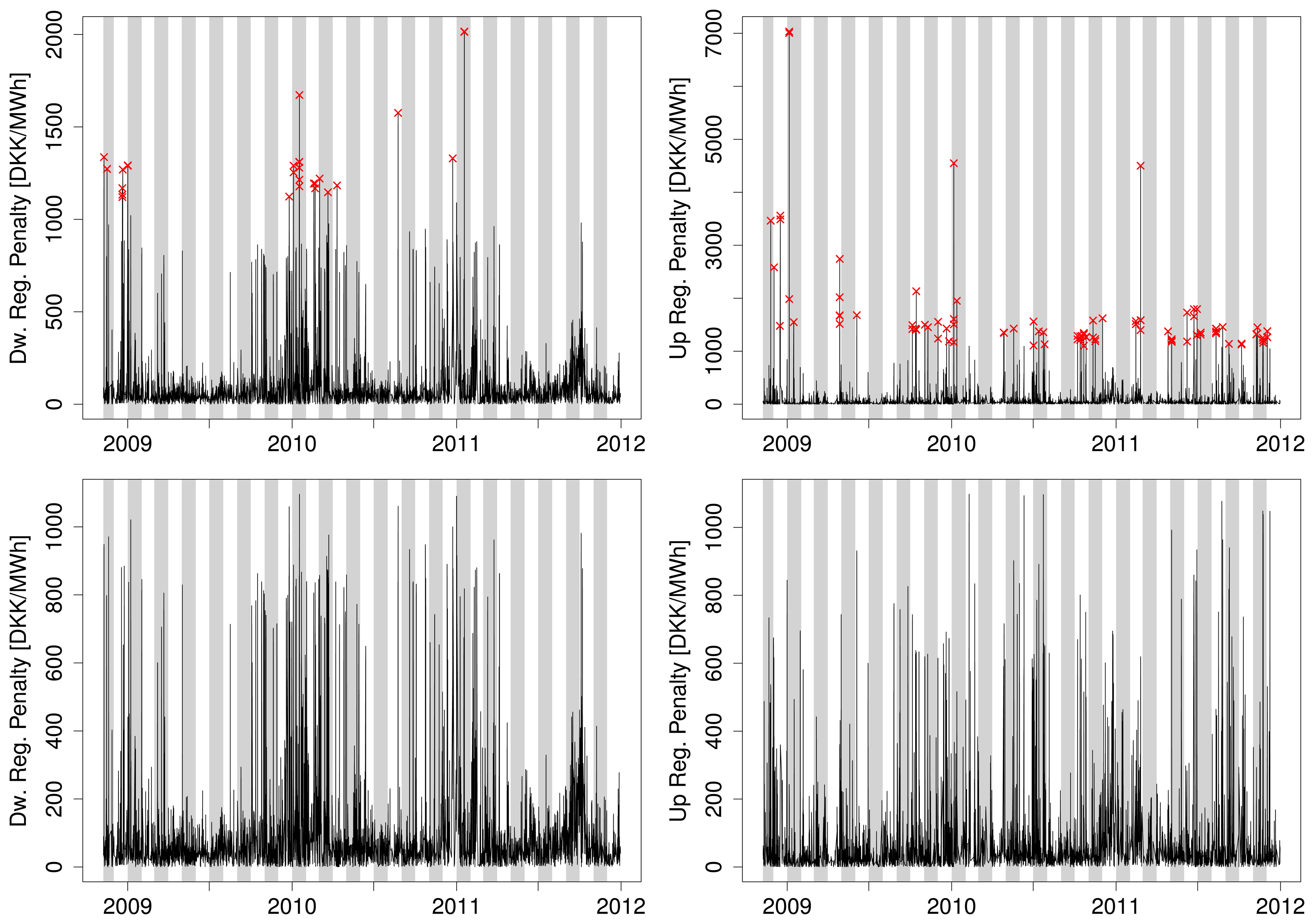
The penalty series, ${\psi }_{t\mid >0}^{((\uparrow /\downarrow ))}$, include a few spikes of such magnitude that they would induce biases in parameter estimates of our statistical models. These extremes are thus removed from the data set after being identified by the procedure described in [22]. The unmodified time series are plotted in the top row of Figure 1, where the removed observations are marked with a cross. In total of 85 and 29 observations was removed from the up- and down-regulation penalty series, respectively.

Cleaned versions of the series are shown in the bottom row of the same figure. They reveal considerable time-variations in the first and second order moments of the penalties. The mean constantly fluctuates, and volatile periods with rather frequent price spikes are followed by periods of relative tranquility.

Table 1. The empirical probabilities of Ī^(↑/↓) over the period analyzed.

↓	∼	↑
39.00%	29.30%	31.70%

summarizes the empirical probabilities, Ī^(↑/↓), for the states of ${\mathit{\text{I}}}_t^{((\uparrow /\downarrow ))}$. It reveals the dominance of down-regulation in long-term expectation, while the other two states' probabilities are quite similar.

Let ${\mathit{Î}}_t^{((\uparrow /\downarrow ))}$ denote the exponentially smoothed average of ${\mathit{I}}_t^{((\uparrow /\downarrow ))}$. At any given time, t, ${\mathit{Î}}_t^{((\uparrow /\downarrow ))}$ is updated with:

$${\mathit{Î}}_t^{((\uparrow /\downarrow ))}=\mathrm{\lambda }{\mathit{I}}_t^{((\uparrow /\downarrow ))}+(1-\mathrm{\lambda }){\mathit{Î}}_{t-1}^{((\uparrow /\downarrow ))}$$

(17)

where 0 < λ < 1 is a smoothing parameter. Should the probabilities of each regulation scenario be constant over the period analyzed, ${\mathit{Î}}_t^{((\uparrow /\downarrow ))}$ would oscillate around its mean Ī^(↑/↓) with deviations inversely related to λ.

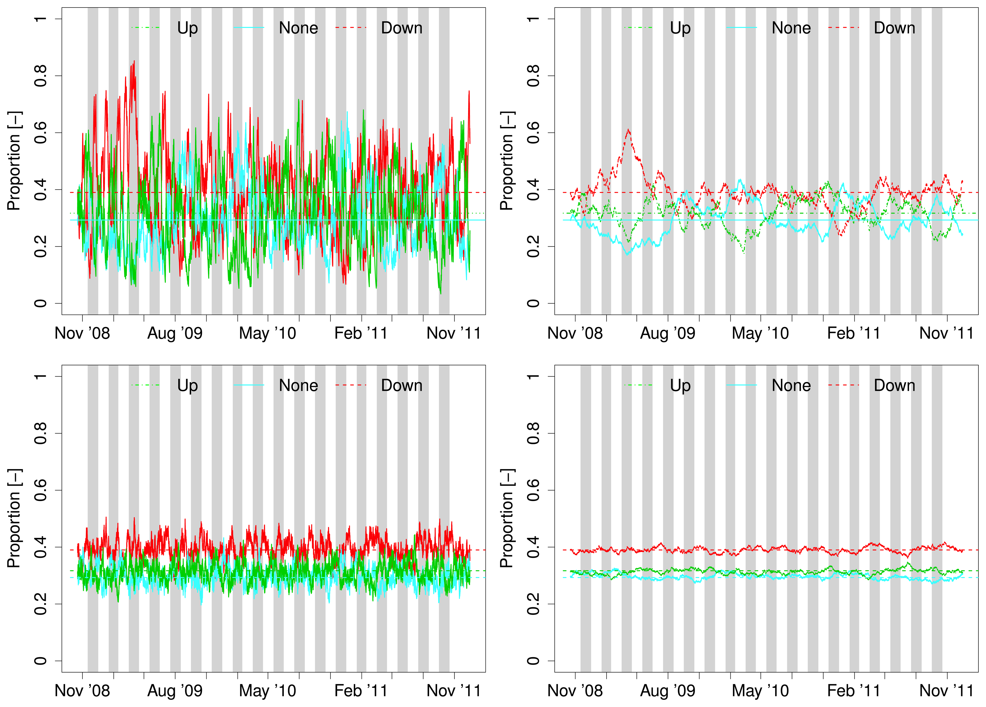
However, as illustrated by Figure 2, this is not the case for the imbalance sign probabilities. The bottom two plots show the tracking of a series simulated from a trinomial distribution with probabilities of each instance equal to the empirical probabilities from Table 1. The top two plots, on the other hand, show the tracking of the actual occurrences of regulation in each direction. Forgetting these factors, λ = 0.99 and λ = 0.999 were applied for the two plots on the left and on the right, respectively.

For both values of λ, the observed series deviate considerably more from the empirical probabilities and seems to drift distinctively away from them over shorter periods. The plots therefore provide a clear indication that greater knowledge about the next day's imbalance sign can be obtained by considering more dynamic approaches to the modeling of such probabilities.

3.3. Seasonality

Mainly driven by the daily and weekly cycles of consumption, electricity prices are generally known to have the same seasonal cycles. It therefore seems natural to examine the seasonalities of ${\mathit{I}}_t^{((\uparrow /\downarrow ))}$ and ${\psi }_{t\mid >0}^{((\uparrow /\downarrow ))}$.

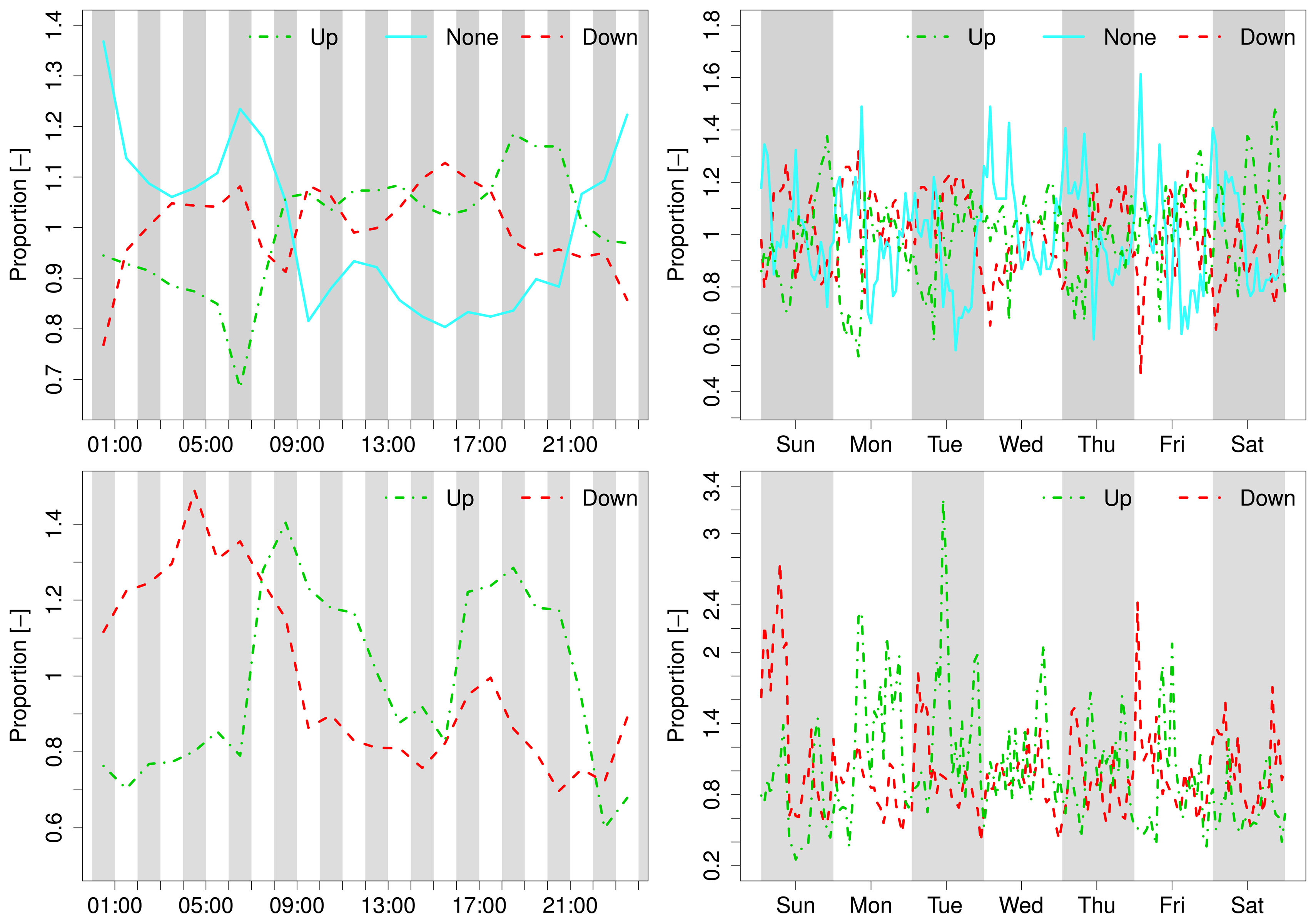
Figure 3 depicts averages of ${\mathit{\text{I}}}_t^{((\uparrow /\downarrow ))}$ and ${\psi }_{t\mid >0}^{((\uparrow /\downarrow ))}$ for each hour of the day and of the week relative to the corresponding empirical means. For the imbalance sign, there is an apparent diurnal variation for the up- and non-regulation hours. For the down-regulation hours, the diurnal variation is less distinctive, yet there seems to be some evidence of such behavior. Furthermore, the frequency of up-regulation hours seems to exhibit stronger diurnal variation during the weekends than during working days, whereas the opposite is observed for the non-regulation hours. The diurnal variation of the frequency of down-regulation hours seems to be quite consistent throughout the week.

Penalties have an obvious diurnal seasonality, where up-regulation penalties are generally above average during the day and below average during the night, while down-regulation penalties exhibit the opposite pattern. Given the high share of hours where ${\psi }_{t\mid >0}^{((\uparrow /\downarrow ))}$ is not defined, segmenting the penalties according to the hour of the week dilutes the data quite severely The excessive fluctuations seen in the bottom-right plot of Figure 3 should therefore be interpreted with caution. Besides magnitude variations, daily seasonal cycles seem to be consistent throughout the entire week.

3.4. Exogenous Variables

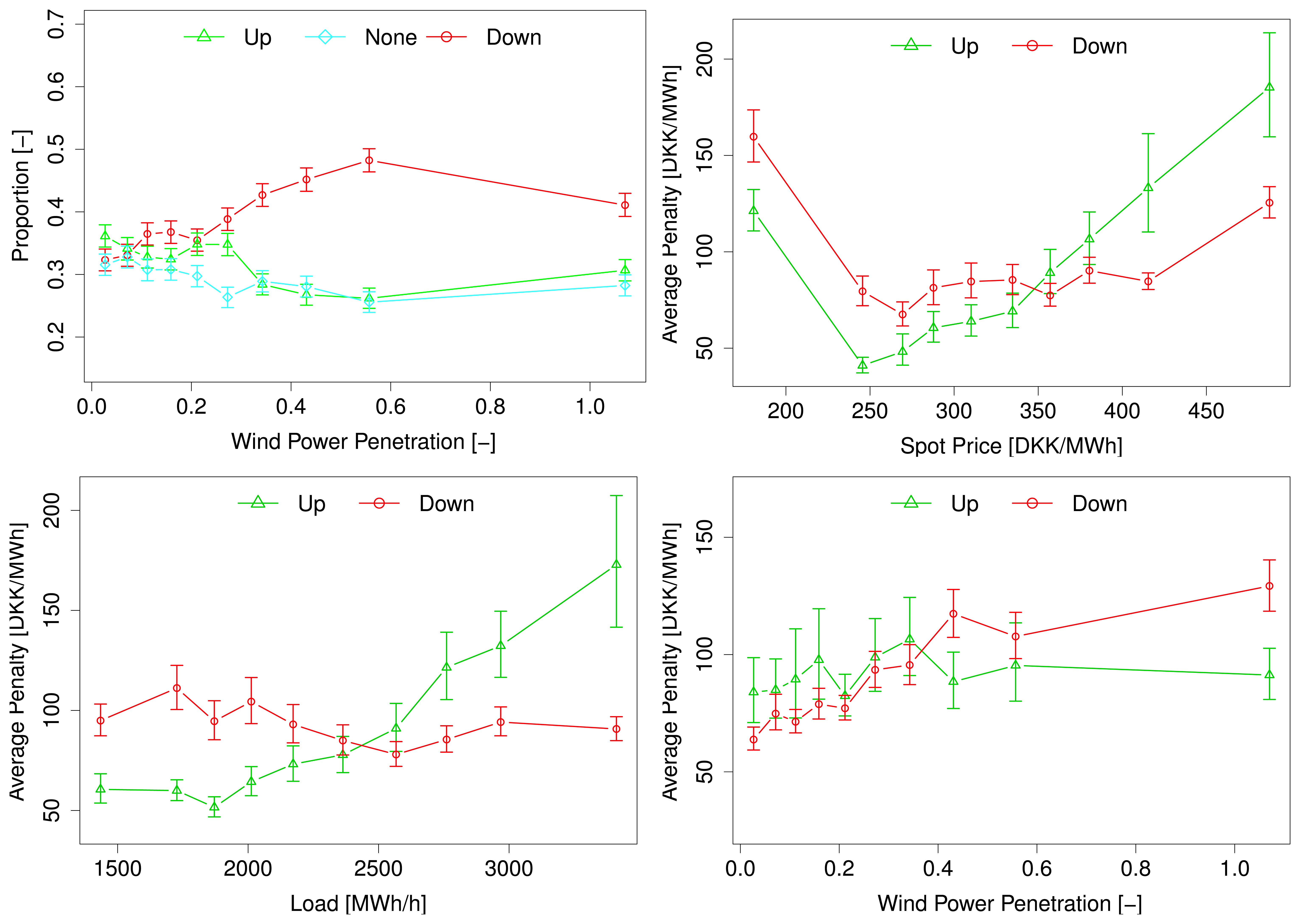
Figure 4 illustrates the impact of exogenous variables deemed relevant for the imbalance sign and penalties. These plots are constructed by segmenting the data into 10 equally populated bins according to x-axis variable. The sign frequency, or average penalty, for each bin is plotted against the bin median. Along with the mean of each bin, 95% confidence intervals obtained by bootstrapping (see [23]) are shown.

The top-left plot in Figure 4 shows the empirical frequencies of each imbalance sign as a function of predicted wind power penetration. Wind power penetration is defined as the ratio between predicted wind power production and predicted load. Our motivation to use such a variable, instead of actual production forecasts, is to account for the varying ability of wind power to affect the market outcome depending upon demand [24]. The remaining three plots in Figure 4 illustrate the dependencies of average imbalance penalties upon predicted spot price (top right), load (bottom left) and wind power penetration (bottom right).

The top-left plot indicates a significant impact of predicted wind power penetration and imbalance sign. besides, the top-right plot shows that both penalties are significantly affected by the predicted spot price. Even though some of the middle points are not so different from their neighbors, there are non-negligible differences between points that are located further apart. Similar conclusions can be drawn for the impact of predicted load on up-regulation penalties and for the impact of predicted wind power penetration on down-regulation penalties. The predicted load, however, does not seem to have an influence on down-regulation penalties. Likewise, up-regulation penalties seem to be merely affected by predicted wind power penetration.

The previously demonstrated dynamic and seasonal variations of ${\mathit{\text{I}}}_t^{((\uparrow /\downarrow ))}$ and ${\psi }_{t\mid >0}^{((\uparrow /\downarrow ))}$ are not taken into account here. This hence prevents any final conclusions to be drawn from the plots. The question of whether or not the imbalance sign and penalties are affected by these variables will be answered by examining whether a model including this information has superior forecasting skills compared to a model that does not account for it.

4. Holt-Winters Model for the Imbalance Sign and Penalties

The Holt-Winters model (HW model) is a pragmatic approach to model seasonal time series. The standard formulation of the HW model, suitable for time series with a single seasonal pattern, was introduced by [13]. In [25], the HW model is extended to accommodate multiple seasonal patterns. The model can be formulated either as an additive or as a multiplicative one. The authors of [26] and [27] provide an excellent overview of these different possible formulations. In light of the vast existing literature on the generalities of HW models, the discussion is limited here to the relevant formulations used at various modeling stages.

4.1. Standard Holt-Winters

For a stochastic process, Y_t = [y₀, y₁,…] for t = [0,1,…], an additive double seasonal HW model without a trend term can be written as:

$${\mu }_t={\alpha }_{\mu }(y_t-(S_{t-s_1}^{(1)}+S_{t-s_2}^{(2)}))+(1-\alpha ){\mu }_{t-1}$$

(18)

$$S_t^{(1)}={\alpha }_{S^{(1)}}(y_t-({\mu }_t+S_{t-s_2}^{(2)}))+(1-{\alpha }_{S^{(1)}})S_{t-s_1}^{(1)}$$

(19)

$$S_t^{(2)}={\alpha }_{S^{(2)}}(y_t-({\mu }_t+S_{t-s_1}^{(1)}))+(1-{\alpha }_{S^{(2)}})S_{t-s_2}^{(2)}$$

(20)

where s₁ and s₂ are the periods of seasonal components S⁽¹⁾ and S⁽²⁾, respectively, while α_μ, α_S⁽¹⁾ and α_S⁽²⁾ are smoothing parameters. After the updating step in Equations (18)–(20), the k-step ahead prediction, ŷ_t+k∣t, is given by:

$${ŷ}_{t+k\mid t}={\mu }_t+S_{t-s_1+k}^{(1)}+S_{t-s_2+k}^{(2)}.$$

(21)

Similarly, a multiplicative HW model for Y_t with two seasonal cycles can be defined as:

$${\mu }_t={\alpha }_{\mu }(y_t/(S_{t-s_1}^{(1)}{S}_{t-s_2}^{(2)}))+(1-\alpha ){\mu }_{t-1}$$

(22)

$$S_t^{(1)}={\alpha }_{S^{(1)}}(y_t/({\mu }_t{S}_{t-s_2}^{(2)}))+(1-{\alpha }_{S^{(1)}})S_{t-s_1}^{(1)}$$

(23)

$$S_t^{(2)}={\alpha }_{S^{(2)}}(y_t/({\mu }_t{S}_{t-s_1}^{(1)}))+(1-{\alpha }_{S^{(2)}})S_{t-s_2}^{(2)}$$

(24)

for which the definitions of s₁ and s₂ are the same as in the above, while:

$${ŷ}_{t\mid t-k}={\mu }_t{S}_{t-s_1+k}^{(1)}{S}_{t-s_2+k}^{(2)}$$

(25)

By defining the one step prediction error as:

$${\epsilon }_{t\mid t-1}=y_t-{ŷ}_{t\mid t-1}$$

(26)

and following [28], the models can be made robust by defining:

$$y_t^{(*)}={ŷ}_{t\mid t-1}+g({\epsilon }_{t\mid t-1},\tau )$$

(27)

where g(·,τ) is the Huber influence function:

$$g(\mu ,\tau )=\{\begin{array}{ll}u\hfill & \text{if}\left|u\right|<=\tau \hfill \\ sgn(u)\tau \hfill & \text{if}\left|u\right|>\tau \hfill \end{array}$$

(28)

and by substituting $y_t^{(*)}$ for y_t in Equations (18)–(20) and Equations (22)–(24).

In compliance with the common formulation of the HW model in the literature, Equations (18)–(20) can be written on their more compact error-correction form as:

$${\mu }_t={\mu }_{t-1}+{\alpha }_{\mu }g({\epsilon }_{t\mid t-1},\tau )$$

(29)

$$S_t^{(1)}=S_{t-s_1}^{(1)}+{\alpha }_{S^{(1)}}g({\epsilon }_{t\mid t-1},\tau )$$

(30)

$$S_t^{(2)}=S_{t-s_2}^{(2)}+{\alpha }_{S^{(2)}}g({\epsilon }_{t\mid t-1},\tau )$$

(31)

It is readily seen that letting τ = ∞ yields a non-robust HW model.

Should a single seasonal pattern be sufficient, Equations (20), (24) and (31) are simply omitted from the models. Correspondingly, the second seasonal term vanishes from the prediction Equations (25) and (21).

4.2. Conditional Holt-Winters Model

In order to account for the effects of external variables, e.g., predicted spot price, wind power penetration and load, the previously described HW models can be conditioned on exogenous variables. Let X_t = [x₀, x₁,…] for t = [0,1,…] be a variable on which Y_t arbitrarily depends. Inspired by [29], let x_i, i ∈ [1,…, M] be a particular fitting point in a set of M distinct fitting points in X_t. At each x_i, a HW model like the ones given either by Equations (22)–(24) or by (29)–(31) can describe the dynamics of Y_t in the close vicinity of x_i. A model fully describing Y_t can then be found as a series of M different HW models each on the same form, as given previously. Now, however, the smoothing in each model at time t is not only done in time, but also by weighting the observations according to the Euclidean distance between x_t and x_i. The weights are assigned as:

$${\upsilon }_{x_i}(x_t)=V\left(\frac{\Vert x_t-{\mathit{x}}_i\Vert }{h({\mathit{x}}_i)}\right)$$

(32)

where V(·) is a function taking non-negative arguments, ‖ · ‖ denotes the Euclidean norm and h(x_i) is the bandwidth applied in the fitting point x_i. Following [29] and [30], a tri-cube kernel used to determine the weights, i.e.,

$$V(u)=\{\begin{array}{ll}{(1-u^3)}^3\hfill & \text{if}u\in [0;1)\hfill \\ 0\hfill & \text{otherwise}\hfill \end{array}$$

(33)

which entails weights between zero and one. A nearest-neighbor bandwidth is employed here. This implies that the actual bandwidth varies with the local density of the data, since h(x_i) is set as the range of the (γ · 100)% closest observation to each x_i, where 0 ≤ γ ≤ 1 is the relative bandwidth, common for all fitting points. Eventually, one defines α = [ α_μ α_S⁽¹⁾ α_S⁽²⁾ ] and subsequently finds the effective smoothing parameters at time t, and for the fitting point x_i, as:

$${\mathit{\alpha }}^{(\mathit{\text{eff}})}(t,i)=\mathit{\alpha }{\upsilon }_{x_i}(x_t)$$

(34)

The robust conditional HW model thus consists of M models, for which the additive version of the updating formulae for the i-th model is:

$${\mu }_{t,i}={\mu }_{t-1,i}+{\alpha }_{\mu }^{(\mathit{\text{eff}})}(t,i)g({\epsilon }_{t\mid t-1},\tau )$$

(35)

$$S_{t,i}^{(1)}=S_{t-s_1,i}^{(1)}+{\alpha }_{S^{(1)}}^{(\mathit{\text{eff}})}(t,i)g({\epsilon }_{t\mid t-1},\tau )$$

(36)

$$S_{t,i}^{(2)}=S_{t-s_2,i}^{(2)}+{\alpha }_{S^{(2)}}^{(\mathit{\text{eff}})}(t,i)g({\epsilon }_{t\mid t-1},\tau )$$

(37)

Similarly, the updating scheme for the i-th multiplicative HW model becomes:

$${\mu }_{t,i}={\alpha }_{\mu }^{(\mathit{\text{eff}})}(t,i)(y_t^{(*)}/(S_{t-s_1}^{(1)}{S}_{t-s_2}^{(2)}))+(1-{\alpha }_{\mu }^{(\mathit{\text{eff}})}(t,i)){\mu }_{t-1,i}$$

(38)

$$S_{t,i}^{(1)}={\alpha }_{S^{(1)}}^{(\mathit{\text{eff}})}(t,i)(y_t^{(*)}/({\mu }_t{S}_{t-s_2}^{(2)}))+(1-{\alpha }_{S^{(1)}}^{(\mathit{\text{eff}})}(t,i))S_{t-s_1}^{(1)}$$

(39)

$$S_{t,i}^{(2)}={\alpha }_{S^{(2)}}^{(\mathit{\text{eff}})}(t,i)(y_t^{(*)}/({\mu }_t{S}_{t-s_1}^{(1)}))+(1-{\alpha }_{S^{(2)}}^{(\mathit{\text{eff}})}(t,i))S_{t-s_2}^{(2)}$$

(40)

For a value of x_t with x_i ≤ x_t ≤ x_i+1, y_t+k∣t is found by linear interpolating between ŷ_t+k∣t,i and ŷ_t+k∣t,i+1.

Although, in principle, the number of variables used to condition upon could be infinity, one should be cautious in doing so, due to the risk of sparse updates in the points located close to the edges of the multidimensional space.

4.3. Parameter Estimation

Let β be the model parameters,

$$\beta =\{\begin{array}{ll}\left[\begin{array}{cc}\mathit{\alpha }& \tau \end{array}\right]\hfill & \text{for the standard HW model}\hfill \\ \left[\begin{array}{ccc}\mathit{\alpha }& \gamma & \tau \end{array}\right]\hfill & \text{for the conditional HW model}\hfill \end{array}$$

(41)

Due to the binary nature of the ${\mathit{I}}_t^{((\uparrow /\downarrow ))}$, only the additive formulation of the HW model is feasible for modeling the imbalance sign. Given N observations of I^(↑/↓), an estimate β can be derived by Maximum Likelihood (ML) estimation,

$$\widehat{\beta }=\underset{\beta }{argmax}\ell (\beta )$$

(42)

where ℓ(β) is the log-likelihood function for a trinomial variable,

$$\ell (\beta )=\sum _{t=1}^N\{I_{t,1}^{(\uparrow /\downarrow )}log{p}_{t,1}(\beta )+I_{t,3}^{(\uparrow /\downarrow )}log{p}_{t,3}(\beta )+(1-(I_{t,1}^{(\uparrow /\downarrow )}+I_{t,3}^{(\uparrow /\downarrow )}))\text{log}(1-p_{t,1}(\beta )-p_{t,3}(\beta ))\}$$

(43)

where, in turn, $p_{t,i}(\beta )=\text{ℙ}(I_{t,i}^{(\uparrow /\downarrow )}=1\mid \beta )$. Since a finite value for τ is not meaningful in the context of binary variables, it is fixed at τ = ∞ for ${\mathit{I}}_{t,i}^{(\uparrow /\downarrow )}$.

After the updating and forecasting steps, the inverse logit-transformation is applied for deriving the posterior probabilities for the imbalance sign,

$${\widehat{\text{ℙ}}}_{t+k\mid t}\left(I_{t+k}^{(\psi )}=-1\right)={\widehat{\text{ℙ}}}_{t+k\mid t}\left(I_{t+k,1}^{(\uparrow /\downarrow )}=1\right)=\frac{exp\left({\mathit{Î}}_{t+k\mid t,1}^{(\uparrow /\downarrow )}\right)}{1+exp\left({\text{∑}}_{i\in \left\{1,3\right\}}{\mathit{Î}}_{t+k\mid t,i}^{(\uparrow /\downarrow )}\right)}$$

(44)

$${\widehat{\text{ℙ}}}_{t+k\mid t}\left(I_{t+k}^{(\psi )}=1\right)={\widehat{\text{ℙ}}}_{t+k\mid t}\left(I_{t+k,3}^{(\uparrow /\downarrow )}=1\right)=\frac{exp\left({\mathit{Î}}_{t+k\mid t,3}^{(\uparrow /\downarrow )}\right)}{1+exp\left({\text{∑}}_{i\in \left\{1,3\right\}}{\mathit{Î}}_{t+k\mid t,i}^{(\uparrow /\downarrow )}\right)}$$

(45)

$$\begin{array}{ll}{\widehat{\text{ℙ}}}_{t+k\mid t}\left(I_{t+k}^{(\psi )}=0\right)& ={\widehat{\text{ℙ}}}_{t+k\mid t}\left(I_{t+k,2}^{(\uparrow /\downarrow )}=1\right)=\frac{1}{1+exp\left({\text{∑}}_{i\in \left\{1,3\right\}}{\mathit{Î}}_{t,i}^{(\psi )}\right)}\\ & =1-\left(\widehat{\text{ℙ}}\left(I_{t+k}^{(\psi )}=-1\right)+\widehat{\text{ℙ}}\left(I_{t+k}^{(\psi )}=+1\right)\right)\end{array}$$

(46)

For the case of regulation penalties, both the multiplicative and the additive formulations of the HW models are tested. The estimation procedure is the same for both models. An estimate of β is found by minimizing the sum of squared residuals, with forecasts forced to be positive,

$$\widehat{\beta }=\underset{\beta }{argmax}{\text{∑}_{i=1}^N\left({\psi }_{i|>0}^{(\uparrow /\downarrow )}-max\{0,{\widehat{\psi }}_{i|>0}^{(\uparrow /\downarrow )}\}\right)}^2$$

(47)

In the estimation process, the practical situation of day-ahead market participation is mimicked. More specifically, the models are fit in the context of forecasts made at 11:00 on the day before realization. Therefore, estimates for the hour between 00:00 and 01:00 are found using k = 13 while k = 37 for the hour between 23:00 and 00:00.

5. Empirical Investigation Results

Various versions of the model described in the previous section are fit to the data in order to conclude on the their most appropriate structure. The first 14 months of the data set (i.e., before 1 January 2010) are used for parameter estimation, and the subsequent two years are seen as an independent test period. In terms of seasonal cycles, the following model structures are tried:

I

Exponential smoothing, i.e., no seasonalities included;

II

Single seasonal HW-model with a daily period, i.e., S⁽¹⁾ = 24;

III

Single seasonal HW-model with a weekly period, i.e., S⁽¹⁾ = 168;

IV

Double seasonal HW-model with daily and weekly periods, i.e., S⁽¹⁾ = 24 and S⁽²⁾ = 168.

Unconditional models are fitted for all three series, as well as conditional ones. For the imbalance penalties, all possible combinations of exogenous variables, i.e., predicted spot price, wind power penetration and load, are evaluated. When it comes to the imbalance sign, however, the model is only conditioned on predicted wind power penetration. For all conditional models, fitting points are chosen as the deciles of the explanatory variables in the training set. Since there are in total 56 different versions of the penalty models tried, results are only presented for a few of the best performing ones.

For all models, only one set of parameters is estimated across all lead times and fitting points. Although this along with the somewhat arbitrarily chosen fitting points might lead to sub-optimal results for individual lead times and fitting points, the obtained results are decisive enough to serve the objective of this paper. Should the model be implemented in practice, however, the extra effort of estimating more locally optimal parameters would most certainly be worthwhile.

5.1. Imbalance Sign Probabilities

For a more intuitive comparison of the models, also for different periods, the discrete ranked probability skill score (RPSS_D) [31] is employed. The RPSS_D is given by:

$$\begin{array}{ll}{\text{RPSS}}_D& =1-\frac{\frac{1}{N}{\text{∑}}_{t=1}^{T_N}{\text{RPS}}_{{\mathit{Î}}_t^{(\uparrow /\downarrow )},t}}{\frac{1}{N}{\text{∑}}_{t=1}^{T_N}{\text{RPS}}_{{\mathit{Ī}}^{(\uparrow /\downarrow )},t}}\\ & =1-\frac{{\text{∑}}_{t=1}^{T_N}{\text{∑}}_{k=1}^3{\left({\text{∑}}_{i=1}^k{\mathit{Î}}_{t,i}^{(\uparrow /\downarrow )}-{\text{∑}}_{i=1}^k{I}_{t,i}^{(\uparrow /\downarrow )}\right)}^2}{{\text{∑}}_{t=1}^{T_N}{\text{∑}}_{k=1}^3{\left({\text{∑}}_{i=1}^k{\mathit{Ī}}_i^{(\uparrow /\downarrow )}-{\text{∑}}_{i=1}^k{I}_{t,i}^{(\uparrow /\downarrow )}\right)}^2+D}\end{array}$$

(48)

where ${\text{RPS}}_{{\mathit{Î}}_t^{(\uparrow /\downarrow )},t}$ and ${\text{RPS}}_{{\mathit{Ī}}^{(\uparrow /\downarrow )},t}$ are the ranked probability scores [32–34] for estimated posterior probabilities, and for climatology forecasts, respectively Furthermore, D is a bias correction term, i.e.,

$$D=\frac{1}{N}\text{∑}_{k=1}^3\text{∑}_{i=1}^k\left[{\mathit{Ī}}_i^{(\uparrow /\downarrow )}\left(1-{\mathit{Ī}}_i^{(\uparrow /\downarrow )}-2\text{∑}_{j=i+1}^k{\mathit{Ī}}_j^{(\uparrow /\downarrow )}\right)\right]$$

(49)

The estimated parameters along with the corresponding RPSS_D are collated in

Table 2. Estimated parameters and RPSS_D for the different model setups investigated.

Model		Model parameters				RPSSD
		γ	αμ	αS(1)	αS(2)	Training set	Test set
Unconditional	I	—	0.0018	—	—	0.5063	0.4796
	II	—	0.0114	0.1161	—	0.5154	0.4815
	III	—	0.0188	—	0.0838	0.5105	0.4778
	IV	—	0.0126	0.1174	0.0626	0.5152	0.4806
Conditional	I	0.9365	0.0022	—	—	0.5052	0.4811
	II	0.9629	0.0090	0.1541	—	0.5141	0.4816
	III	0.8837	0.0203	—	0.0924	0.5072	0.4778
	IV	0.9886	0.0104	0.1460	0.0608	0.5140	0.4808

.

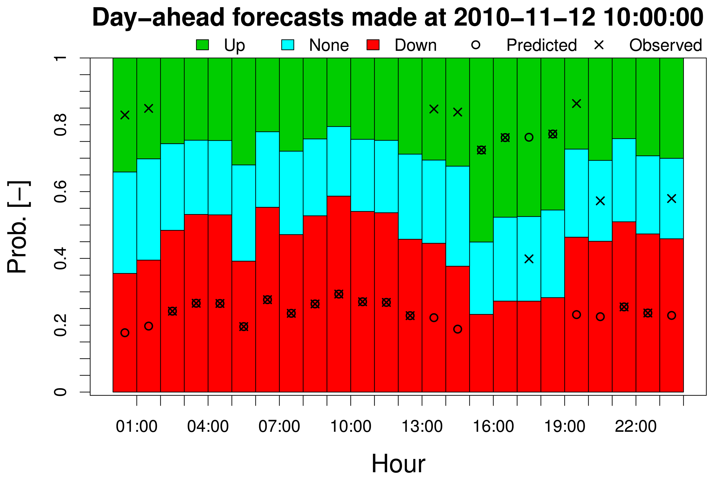
First and foremost, the score values in Table 2 reveal that all models have a forecast skill significantly superior to the constant probability model, since all RPSS_s are considerably higher than zero. The difference in forecast skill between the conditional models and the unconditional ones seems to be insignificant. Considering results over both training and evaluation sets, it appears that the models with daily seasonality are slightly better than the others. The performance of all models with seasonal terms is rather similar, though. For illustration, a visualization of a single set of forecasts is given in Figure 5.

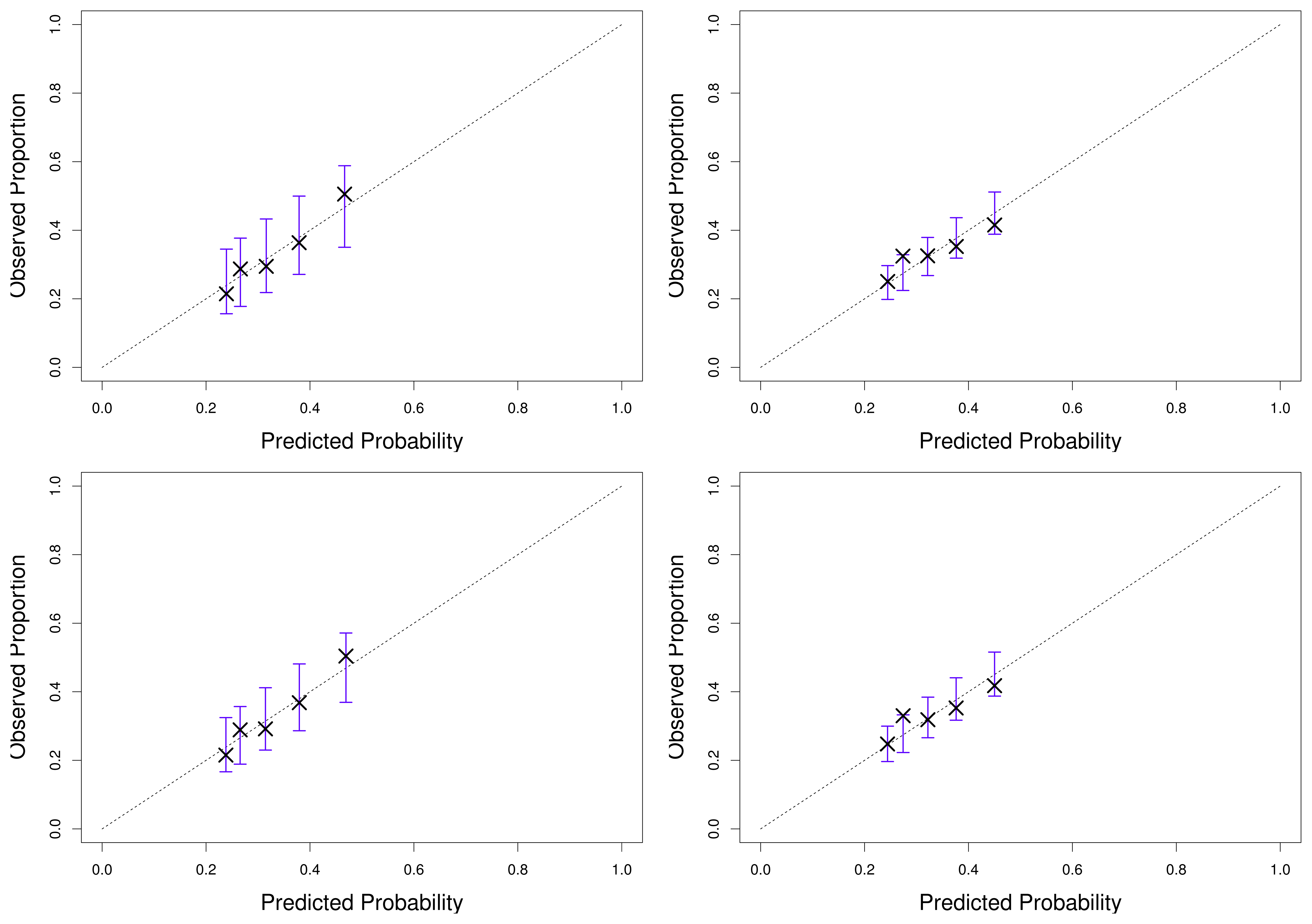
In Figure 6, reliability diagrams for both unconditional and conditional versions of Model II are depicted, along with 95% consistency bars (following the terminology of [35]). The diagrams are based on segmenting predicted probabilities into five equally populated bins centered on their respective averages. The consistency bars are constructed by bootstrapping 10,000 samples with replacement for each bin [23,35,36], accounting for the autocorrelation of the probability transformation integral (PIT), following the proposal of [37].

For both models and periods, the predictions cannot be deemed probabilistically unreliable at the 5% significance level. Both unconditional and conditional models appear to perform similarly overall. Hence, it must be concluded that the forecast wind power penetration has no significant impact on the imbalance sign; at least, not when defined in terms of price differences and under such a family of models.

The reason for the lack of improved forecasting skill most likely lies in the time variation of imbalance sign probabilities; both periodical variations and drift. Since they are not taken into account in Figure 4, the increased probability of down-regulation could be the result of generally higher wind power penetration during the night, while periods of high down-regulation frequency coincide with periods of high wind power production.

As a final remark, it should be noted that the segmentation of predicted probabilities implies that their position in the horizontal dimension is subject to uncertainty just as their vertical position. Especially this uncertainty could be large for the bins, including the highest and the lowest probabilities, as the distribution of elements in these bins is likely to be skewed, positively and negatively, respectively. This property could, however, only inflate the reliability uncertainty and, thus, cannot impact our conclusions. Although an interesting problem, the construction of these two-dimensional consistency bars is beyond the scope of this paper.

5.2. Imbalance Penalties

The imbalance penalty forecasts are evaluated in terms of the root mean square error (RMSE),

$$\text{RMSE}=\sqrt{\frac{{\text{∑}}_{t=1}^N{\left({\psi }_t^{(\uparrow /\downarrow )}-{\widehat{\psi }}_t^{(\uparrow /\downarrow )}\right)}^2}{N}}$$

(50)

and in terms of the R² measure,

$$R^2=1-\frac{{\text{∑}}_{t=1}^N{\left({\psi }_t^{(\uparrow /\downarrow )}-{\widehat{\psi }}_t^{(\uparrow /\downarrow )}\right)}^2}{{\text{∑}}_{t=1}^N{\left({\psi }_t^{(\uparrow /\downarrow )}-{\overline{{\psi }^{(\uparrow /\downarrow )}}}_t\right)}^2}$$

(51)

where ${\overline{{\psi }^{(\uparrow /\downarrow )}}}_t$ is the empirical mean of the penalties during the period considered. Thus, similarly to the case of RPSS_D, the R² measures the relative improvement in forecasting skill compared to the climatological models. For the sake of comparison,

Table 3. Standard deviation of the down- and up-regulation penalties.

Period	Down	Up
Training	109.81	97.56
Test	135.85	118.73

gathers the standard deviations of the time series themselves.

Table 4. The estimated model parameters along with performance measures for the best performing up-regulation penalty models. In-sample measures are for the training set, and out-of-sample ones relate to the test set.

Seasonality	Xt	γ	τ	αμ	αS(1)	In-Sample		Out-of-Sample
						RMSE	R2	RMSE	R2
	π(S) & L	0.2647	793	0.0082	—	92.68	0.0974	116.93	0.0301
Additive	L	0.5372	625	0.0028	0.0447	91.93	0.1120	116.87	0.0311
	π(S) & L	0.5223	701	0.0030	0.0533	92.87	0.0938	114.47	0.0705
Multiplicative	π(S) & L	0.4252	695	0.0050	0.0202	93.57	0.0801	117.13	0.0268

and

Table 5. The estimated model parameters along with performance measures for the best performing down-regulation penalty models. In-sample measures are for the training set, and out-of-sample ones relate to the test set.

Seasonality	Xt	γ	τ	αμ	αS(1)	In-Sample		Out-of-Sample
						RMSE	R2	RMSE	R2
	—-	—	1197	0.0040	—	108.46	0.0243	133.07	0.0405
Additive	—	—	599	0.0022	0.0465	107.22	0.0466	132.35	0.0508
	π(S)	0.9634	74	0.0005	0.1419	110.18	−0.0067	133.15	0.0393
	π(S) & W	0.4491	584	0.0007	0.1523	106.52	0.0590	129.24	0.0948
	π(S) & L	0.6975	611	0.0006	0.0936	107.30	0.0452	131.04	0.0695
	—	—	600	0.0023	0.0451	106.51	0.0592	132.10	0.0544
Multiplicative	π(S) & W	0.3768	574	0.0418	0.0587	106.38	0.0614	129.59	0.0900

list the estimated model parameters, as well as the corresponding performance measures for these up- and down-regulation penalty models.

The best performing models are the conditional ones, more precisely those involving conditioning upon predicted spot price. Moreover, the models include either a mean term only or both mean and daily seasonal terms. However, none of these models performs particularly well: their residual RMSE is only slightly less than the series standard deviation. In light of the optimal smoothing parameters, which yield long model memory, this is not surprising.

The long memory, combined with the high value of τ and the residual RMSE values, indicates that the model is only capable of tracking the relatively long-term average penalty and its variations. Spiking behavior remains undescribed though. This suggest that such behavior is mainly explained by factors that become known after the clearing of the day-ahead market. It would therefore be interesting to estimate expected penalties based on scenarios for some of these factors expected to impact regulation penalties, e.g., wind power and load forecasting errors, as well as remaining capacity on the interconnections to neighboring areas.

5.3. Unconditional Expected Imbalance Penalties

Finally, the models' ability to provide optimal quantile values for the design of optimal wind power offering strategies is examined. Now, recall that the bid that optimizes the hourly expected revenue of a price taking wind power producer is the q̂-quantile of the cdf for wind power generation, where:

$$\widehat{q_t}=\frac{{\widehat{\psi }}_t^{(\downarrow )}}{{\widehat{\psi }}_t^{(\downarrow )}+{\widehat{\psi }}_t^{(\uparrow )}}$$

(52)

and with ${\widehat{\psi }}_t^{(\downarrow )}$ and ${\widehat{\psi }}_t^{(\uparrow )}$, the unconditional expectations for the penalties, given by Equations (11) and (12), respectively.

The market design implies that the realization of q is a binary number for the hours where imbalances in either direction are penalized. For hours when imbalances are not penalized, q is not defined, as it implies division by zero. However, during these hours, any bid between zero and full production can be seen as the correct one. Therefore, q is defined as:

$$q_t=\frac{{\psi }_t^{(\downarrow )}}{{\psi }_t^{(\downarrow )}+{\psi }_t^{(\uparrow )}}=\{\begin{array}{ll}1& \text{if}{\psi }_t^{(\downarrow )}>0\\ 0& \text{if}{\psi }_t^{(\uparrow )}>0\\ \text{Undefined}& \text{if}{\psi }_t^{(\downarrow )}={\psi }_t^{(\uparrow )}=0\end{array}$$

(53)

In order to evaluate the quality of q̂_T, the RPSSD (Equation (48)) is calculated for the hours when q_t is defined during the test period. The climatology model for q is used as the benchmark. This implies that the optimal quantile estimate q̅ is constant throughout the period and found by replacing ${\widehat{\psi }}_t^{(\uparrow /\downarrow )}$ by the period averages in Equation (52). The estimate of q̂ is found using: (i) the unconditional model with a daily seasonal cycle for ${\mathit{Î}}_t^{(\uparrow /\downarrow )}$; (ii) the model conditioned upon the predicted spot price and wind power penetration for ${\widehat{\psi }}_{t\mid >0}^{(\downarrow )}$; and (iii) the model conditional to both the predicted spot price and load for ${\widehat{\psi }}_{t\mid >0}^{(\uparrow )}$. This yields RPSS D = 0.2954, hence indicating that the proposed model outperforms the empirical unconditional probability by a substantial margin.

6. Conclusions and Discussion

Our work has shown that the analysis of real-time electricity markets can significantly improve by building models aiming to described short-term variations in market dynamics. This may be beneficial in both the design of offering strategies and in the appraisal of potential profitability if gaming electricity markets. Despite the fact that our empirical results are somewhat area specific, a number of relevant similarities between the specifics of the Nord Pool and of other electricity markets suggests that similar results would be obtained for other markets, as well.

Our results were derived in a framework tailored for the day-ahead offering of wind power, with its specific lead times (between 13 and 37 hours ahead). Even though conditioning models upon predicted wind power penetration did not result in significant improvements, the conditional Holt–Winters framework is likely to be more relevant for other variables and for shorter lead times. For instance, one interesting aspect to investigate in the context of short-term prediction would be to include updated wind power and load forecasts when they become available.

Although the forecasting skill of the proposed models might seem low to some readers, one has to bare in mind that the process it describes is mainly driven by errors from well-tuned forecasting models and unforeseeable events, like plant malfunctions. Consequently, the observed forecasting quality is, in our opinion, quite satisfactory. From the market operator's point of view, however, the results of this paper might be worrying, since they hint that profitable gaming on the electricity market is possible. Thus, it is clear that anti-gaming policies have to be revised if the desire is to maintain a gaming-free market. Given the current carbon emission curbing targets in various parts of the world, however, the potential benefits of gaming for producers of and systems highly penetrated with electricity by renewable sources have to be considered while structuring such reforms.

The models presented in this paper are adapted to the purpose of facilitating the bidding strategy in the spirit of those presented in [4]. Thus, expectations for imbalance penalties are modeled conditional on the information available before gate closure only. The proposal of similar models for scenario generation purposes does not necessarily call for such availability restrictions. In that case, models can be constructed based on realizations of the variables affecting the penalties, e.g., spot price, regulation needs and interconnection capacity to neighboring areas. In that case, accounting for the interdependence between simulated variables becomes paramount, for instance using the method presented in [38].

References

- Bremnes, J.B. Probabilistic wind power forecasts using local quantile regression. Wind Energy 2004, 7, 47–54. [Google Scholar]
- Matevosyan, J.; Söder, L. Minimization of imbalance cost trading wind power on the short-term power market. IEEE Trans. Power Syst. 2006, 21, 1396–1404. [Google Scholar]
- Pinson, P.; Chevallier, C.; Kariniotakis, G.N. Trading Wind Generation From Short-Term Probabilistic Forecasts of Wind Power. IEEE Trans. Power Syst. 2007, 22, 1148–1156. [Google Scholar]
- Zugno, M.; Jónsson, T.; Pinson, P. Trading wind energy based on probabilistic forecasts of wind generation and market quantities. Wind Energy 2013, 16, 909–926. [Google Scholar]
- Morales, J.M.; Conejo, A.J.; Pérez-Ruiz, J. Short-term trading for a wind power producer. IEEE Trans. Power Syst. 2010, 25, 554–564. [Google Scholar]
- Gibescu, M.; Kling, W.L.; van Zwet, E.W. Bidding and regulating strategies in a dual imbalance pricing system: Case study for a Dutch wind producer. Int. J. Energy Technol. Policy 2008, 6, 240–253. [Google Scholar]
- Galloway, S.; Bell, G.; Burt, G.; McDonald, J.; Siewerski, T. Managing the risk of trading wind energy in a competitive market. IEE Gener. Transm. Distrib. 2006, 153, 106–114. [Google Scholar]
- Rahimiyan, M.; Morales, J.M.; Conejo, A.J. Evaluating alternative offering strategies for wind producers in a pool. Appl. Energy 2011, 88, 4918–4926. [Google Scholar]
- Skytte, K. The regulating power market on the Nordic power exchange Nord Pool: An econometric analysis. Energy Econ. 1999, 21, 295–308. [Google Scholar]
- Gneiting, T. Quantiles as optimal point forecasts. Int. J. Forecast. 2010, 27, 197–207. [Google Scholar]
- Boogert, A.; Dupont, D. On the effectiveness of the anti-gaming policy between the day-ahead and real-time electricity markets in The Netherlands. Energy Econ. 2005, 27, 752–770. [Google Scholar]
- Olsson, M.; Söder, L. Modeling real-time balancing power market prices using combined SARIMA and Markov processes. IEEE Trans. Power Syst. 2008, 23, 443–450. [Google Scholar]
- Winters, P.R. Forecasting sales by exponentially weighted moving averages. Manag. Sci. 1960, 6, 324–342. [Google Scholar]
- Nord Pool Spot AS. Exchange Information 2009. Available online: http://nordpoolspot.com (accessed on 15 March 2014).
- Nord Pool Spot AS. Exchange Information 2010. Available online: http://nordpoolspot.com (accessed on 15 March 2014).
- Nord Pool Spot AS. Exchange Information 2011. Available online: http://nordpoolspot.com (accessed on 15 March 2014).
- Nord Pool Spot AS. The Power Market - How does it work? http://nordpoolspot.com (accessed on 15 March 2014).
- Jónsson, T.; Pinson, P.; Madsen, H. Forecasting electricity spot prices accounting for wind power predictions. IEEE Trans. Sustain. Energy 2013, 4, 210–218. [Google Scholar]
- Nielsen, T.S.; Nielsen, H.A.; Madsen, H. Prediction of wind power using time-varying coefficient functions. Proceedings of 15th Triennial World Congress of the International Federation of Automatic Control, Barcelona, Spain, 21–26 July 2002.
- Lange, M. On the uncertainty of wind power predictions—Analysis of the forecast accuracy and statistical distribution of errors. J. Sol. Energy Eng. Trans. ASME 2005, 127, 177–184. [Google Scholar]
- Jónsson, T.; Ryan, S.M.; Zugno, M.; Pinson, P. Risk Averse Bidding of Wind Fower: Formulation and Properties; Technical report 2012-03; Department of Applied Mathematics and Computer Science, Technical University of Denmark: Kgs. Lyngby, Denmark; 15; April; 2012. [Google Scholar]
- Jónsson, T. Forecasting and decision-making in electricity markets with focus on wind energy. Ph.D. thesis, Department of Applied Mathematics and Computer Science, Technical University of Denmark, Kgs. Lyngby, Denmark, 25 July 2012. [Google Scholar]
- Efron, B.; Tibshirani, R. Bootstrap methods for standard errors, confidence intervals, and other measures of statistical accuracy. Stat. Sci. 1986, 1, 54–77. [Google Scholar]
- Jónsson, T.; Pinson, P.; Madsen, H. On the market impact of wind energy forecasts. Energy Econ. 2010, 32, 313–320. [Google Scholar]
- Taylor, J.W. Short-term electricity demand forecasting using double seasonal exponential smoothing. J. Oper. Res. Soc. 2003, 54, 799–805. [Google Scholar]
- Hyndman, R.J.; Koehler, A.B.; Ord, J.K.; Snyder, R.D. Forecasting with Exponential Smoothing—The State Space Approach; Springer: New York, NY, USA, 2008. [Google Scholar]
- Hyndman, R.J.; Koehler, A.B.; Snyder, R.D.; Grose, S. A state space framework for automatic forecasting using exponential smoothing methods. Int. J. Forecast. 2002, 18, 439–454. [Google Scholar]
- Gelper, S.; Fried, R.; Croux, C. Robust forecasting with exponential and Holt-Winters smoothing. J. Forecast. 2010, 29, 285–300. [Google Scholar]
- Cleveland, W.S.; Devlin, S.J. Locally Weighted Regression: An Approach to Regression Analysis by Local Fitting. J. Am. Stat. Assoc. 1988, 83, 596–610. [Google Scholar]
- Nielsen, H.A.; Nielsen, T.S.; Joensen, A.K.; Madsen, H.; Holst, J. Tracking time-varying coefficient functions. Int. J. Adapt. Control Signal Process. 2000, 14, 813–828. [Google Scholar]
- Weigel, A.P.; Liniger, M.A.; Appenzeller, C. The discrete Brier and ranked probability skill scores. Mon. Weather Rev. 2007, 135, 118–124. [Google Scholar]
- Epstein, E. A scoring system for probability forecasts of ranked categories. J. Appl. Meteorol. 1969, 8, 985–987. [Google Scholar]
- Murphy, A.H. On the ranked probability skill score. J. Appl. Meteorol. 1969, 8, 988–989. [Google Scholar]
- Murphy, A.H. A note on the ranked probability skill score. J. Appl. Meteorol. 1971, 10, 155–156. [Google Scholar]
- Broecker, J.; Smith, L.A. Increasing the reliability of reliability diagrams. Weather Forecast. 2007, 22, 651–661. [Google Scholar]
- Atger, F. Estimation of the reliability of ensemble-based probabilistic forecasts. Q. J. R. Meteorol. Soc. 2004, 130, 627–646. [Google Scholar]
- Pinson, P.; McSharry, P.; Madsen, H. Reliability diagrams for nonparametric density forecasts of continuous variables: accounting for serial correlation. Q. J. R. Meteorol. Soc. 2010, 136, 77–90. [Google Scholar]
- Pinson, P.; Papaefthymiou, G.; Klockl, B.; Nielsen, H.A.; Madsen, H. From probabilistic forecasts to statistical scenarios of short-term wind power production. Wind Energy 2009, 12, 51–62. [Google Scholar]