Optimization Models and Methods for Demand-Side Management of Residential Users: A Survey

Abstract
: The residential sector is currently one of the major contributors to the global energy balance. However, the energy demand of residential users has been so far largely uncontrollable and inelastic with respect to the power grid conditions. With the massive introduction of renewable energy sources and the large variations in energy flows, also the residential sector is required to provide some flexibility in energy use so as to contribute to the stability and efficiency of the electric system. To address this issue, demand management mechanisms can be used to optimally manage the energy resources of customers and their energy demand profiles. A very promising technique is represented by demand-side management (DSM), which consists in a proactive method aimed at making users energy-efficient in the long term. In this paper, we survey the most relevant studies on optimization methods for DSM of residential consumers. Specifically, we review the related literature according to three axes defining contrasting characteristics of the schemes proposed: DSM for individual users versus DSM for cooperative consumers, deterministic DSM versus stochastic DSM and day-ahead DSM versus real-time DSM. Based on this classification, we provide a big picture of the key features of different approaches and techniques and discuss future research directions.1. Introduction
Traditional power grids were designed to supply energy produced by a few central generators connected to the high voltage (HV) network. Nowadays, this scenario is changing because of the remarkable growth of medium- to small-sized renewable energy source (RES) plants, such as hydroelectric, solar and wind, distributed on medium and low voltage (MV and LV) grids. According to [1], the contribution of RESs to the world’s electricity generation in 2010 was about 19% of total global electricity consumption, a considerable increase with respect to previous years. In the European Union, for example, a total of about 58.8 GW of new power capacity was constructed in 2010, and the renewable share of new power installations was 40% [2]. The widespread diffusion of RESs is motivated by the substantial socio-economic benefits obtainable with these sources: reduction of greenhouse gas emissions and air pollution, diversification of energy supply, diminished dependence on imported fuels, economic development and jobs in manufacturing, installation and management of RESs plants [3,4]. Despite these obvious benefits to the environment, industry and consumers themselves, there are some barriers that can limit renewable sources’ penetration [5]. In fact, renewable generation is variable, uncertain and is just partially dispatchable. For this reason, the energy dispatching is much more challenging than in the past, and new instruments are required to ensure the real-time balancing between demand and supply.
In addition to RESs penetration, traditional power grids face also other challenges that limit their efficiency among which are the non-optimal dimensioning and usage of grid resources. In fact, in order to match customers’ demand of electric energy, installed generation, transmission and distribution capacities must be able to meet the peak of demand. Moreover, sufficient additional capacity must be available to deal with the uncertainty in generation and consumption. As a consequence, grids resources are underutilized for most of the time.
Smart grids (SGs) are the new generation of power grids, which have been introduced to address the main issues of traditional grids. Specifically, SGs can make grids more efficient and smarter by means of facilitating the deployment of renewable energy sources, decreasing oil consumption by reducing the need for inefficient generation during peak usage periods, optimizing resources utilization and construction of back-up (peak load) power plants and enabling the integration of plug-in electric vehicles (PEVs) and energy storage systems (ESSs) [6]. In order to properly design these new generation grids, a reference model has been defined, which consists of seven functional blocks, which are, namely, bulk generation, transmission, distribution, operation, market, service provider and customers [6]. The bulk generation domain generates energy by using resources like oil, coal, nuclear fission and RESs and stores electricity to manage the variability of renewable resources. The energy produced is dispatched through the transmission and distribution sectors, which are controlled by the operation domain. The balance between supply and the demand is guaranteed by the market domain, which consists of suppliers of bulk electricity, retailers who supply electricity to users and traders who buy electricity from suppliers and sell it to retailers and aggregators of distributed small-scale power plants. The service provider manages services for utilities companies and end-users, like billing and consumers’ account management. Finally, customers consume energy, but can also generate and store electricity locally. This domain includes residential, commercial and industrial customers, who can actively contribute to the efficiency of the grid.
The residential sector is expected to play a key role in the smart grid framework, since it is currently one of the major contributors to countries’ energy balances [7]. Furthermore, in the near future, residential energy consumption will probably exceed 40% of the total yearly consumption in most of the Western countries [8]. A key feature of consumer demand is that it varies notably depending on the time of day [9] and on the climate [10,11]. Moreover, it is largely uncontrollable and totally inelastic with respect to the power grid conditions (i.e., the energy demand is just partially responsive to prices). To address this issue, demand management mechanisms can be used to optimally manage the energy resources of users and their energy demand profile, with the aim of not only reducing their bills or saving energy, but also using the energy itself more efficiently by means of shifting loads to off-peak hours, adapting the demand to renewable sources’ supply or reacting to emergency conditions. To this purpose, a pivotal role is played by the smart grid information and technologies (IT) infrastructure, which can provide a huge amount of data to consumers, such as real-time information on energy prices, power grid status, renewable sources generation and electric devices consumption.
Demand management mechanisms can be classified into two main categories: demand-response (DR) and demand-side management (DSM). DR methods are reactive solutions designed to encourage consumers to dynamically change their electricity demand in the short term, according to signals provided by the grid/utilities, such as prices or emergency condition requests. Typically, these techniques are used to reduce the peak demand or to avoid system emergencies, such as blackouts. On the other hand, DSM is a proactive approach aimed at making consumers energy-efficient in the long-term. In the literature, demand-response and demand-side management terms are often used as synonymous or misused. Thus, in some works on DSM, proposed solutions are called DR methods and vice-versa. Actually, demand-response and demand-side management are two different methodologies, which can also be used in conjunction with each other.
Demand management mechanisms can be designed to control the electric resource of individual users. However, this approach may have some undesirable effects [12]. In fact, consumers are characterized by a natural diversity in terms of appliance usage. This feature is fully exploited by the power system to optimize its efficiency in generating and distributing energy. Demand management mechanisms for individual users may actually disturb this diversity. In the case of systems for consumers’ payment reduction, for example, all users would shift their loads to periods of the day where the electricity prices are low. Unfortunately, this would determine large peaks of demand during such low-cost periods and, possibly, service interruptions (i.e., blackout or brownouts). To contain these unwanted side-effects, management mechanisms can be designed to control the community of users, thus managing their resources based on a system-wide perspective. Two different approaches are proposed in the literature to define these methods: optimization and game theory. In the first case, all consumers are supposed to cooperate in managing their resources, and optimization models are used to minimize a shared utility function. However, these solutions do not incorporate conflicts among users. In the case of real-time tariffs, for example, energy prices depend on the overall users’ demand, and one consumer’s actions directly affect the others in terms of costs. As a consequence, minimizing the overall bill may be unfair in terms of payment sharing among customers. In order to address conflicts, game theory is usually used, since it can model complex interactions among the independent rational players of the power grid [13].
The natural extension of demand management mechanisms for communities of users is represented by techniques designed for microgrids, which are small-scale versions of the electricity systems that locally generate and distribute electricity to consumers. These grids are an ideal way to integrate renewable resources at the community level and allow for customer participation in the electricity market [14–16].
Although a few surveys have been proposed in the literature in reference to the research challenges of smart grids, optimization techniques for DSM have never been reviewed. For this reason, in this work, we provide a survey of the most relevant studies concerning the optimization of energy resources of users, with a special focus on solutions for residential consumers. Specifically, we review the related literature according to three different contrasting characteristics, which are DSM for individual users versus DSM for cooperative consumers, deterministic DSM versus stochastic DSM and day-ahead DSM versus real-time DSM. Based on these classifications, we seek to provide a clear picture of the strengths and challenges of different approaches and techniques used in designing DSM systems.
The remainder of this paper is organized as follows. Section 2 presents the fundamentals of DSM frameworks, with a special focus on the architectures and approaches used in designing these systems. Section 3 provides a comprehensive formulation of the optimization model, which can be used to describe demand-side management problems. Section 4 surveys DSM models and methods designed to individually manage residential users, while Section 5 reviews DSM mechanisms for cooperative communities of consumers. Finally, Section 6 summarizes this work and identifies future research directions.
2. Fundamentals of Demand-Side Management
In this section, we present the basic architecture and components of DSM frameworks. Moreover, we also provide a broad classification of approaches and optimization techniques for demand-side management. For the ease of presentation, we list in Table 1 the main DSM-related acronyms used in this paper.
2.1. Architecture and Components of DSM Frameworks
Demand-side management frameworks are designed to optimally manage the electric resources of users through a specific architecture, shown in Figure 1, composed of the following basic components:
Local generators: local energy plants (e.g., photovoltaic (PV) plants) that generate electric energy that can be either used locally or injected into the grid.
Smart devices: electric appliances that are able to monitor themselves, thus providing data, such as their energy consumption, and that can be remotely controlled [17].
Sensors: used to monitor several data of interest, such as the user’s position within the house, temperature and light [18]. Moreover, in the case of traditional devices, power meter sensors [19] can be used to monitor and control these appliances.
Energy storage systems: are storage devices that allow the DSM system to be flexible in managing electric resources.
Energy management unit (EMU): exchanges information with the other elements of the system and manages the electric resources of users based on an intelligent DSM mechanism. Specifically, this mechanism has to define the schedule of appliances, the operating plan of ESSs and the demand and supply profiles (i.e., when to buy and inject energy into the grid). In the case of multi-user architectures, all of the EMUs of users are connected to a central server, which coordinates the consumers.
Smart grid domains: the distribution, operation, market, service provider and customer domains of the smart grid described in Section 1. A utility company, which is part of the market domain, supplies electric energy to users from whom it receives payments according to energy tariffs. Eventually, also, a profit-neutral entity, called the independent system operator (ISO), can be introduced, which stands between suppliers and customers. The ISO procures electricity from suppliers and sells it to users with the goal of matching supply and demand.
All of the components of the architecture are connected through a communication infrastructure. Specifically, one or more home area networks (HANs) are used to interconnect the elements that are within the customer’s domain. Several technologies can be used to implement HANs, which can be either wired or wireless [20]. Among wired networks, Ethernet [21] represents a very popular solution, since it allows one to create high-rate HANs (i.e., up to hundreds of Gbps). However, this technology requires investments for the cable deployment. A cheaper alternative is represented by power line communication solutions, which do not need the installation of dedicated cables, since they use power transmission wires. These lines can indeed be utilized to both distribute energy and transmit data with rates in the order of Mbps [22]. Cable deployment is also not required with wireless technologies, such as Wi-Fi [23]. However, wireless solutions generally provide comparatively short distance connections with low data rates, since they are subject to transmission attenuation and environmental interference. Among wireless technologies, wireless sensor networks, such as ZigBee [24] and 6LoWPAN [25] networks, represent a valid alternative, since they can be utilized to create low-cost, flexible, highly-reliable and self-healing communication infrastructures.
In addition to home networks, also wide are networks (WANs) are required to connect EMUs to the other domains of the smart grid, such as the utility company or the central server in the case of DSM solutions for communities of cooperative users. Among the technologies that can be used to implement this communication infrastructure, cellular networks represent a promising solution [26], since they can support large numbers of simultaneous connections with high service coverage. Furthermore, 4 G technologies, such as WiMAX [27] and Long Term Evolution (LTE) [28], can also guarantee reliability and quality of service in data transmission [29].
2.2. Classification of Approaches and Optimization Techniques for DSM
Optimization methods for demand-side management can be classified based on three main characteristics, as summarized in Figure 2. Firstly, DSM systems can be designed to optimize the usage of electric resources of either individual users or a community of cooperative consumers. In the first case, users are individually managed, while in the second case, consumers collaborate in defining their operating plans and DSM methods are used to optimize a shared utility function. A further classification can be obtained based on whether deterministic or stochastic techniques are utilized to design the demand management mechanism. In fact, several parameters of DSM systems, such as RESs’ energy generation, devices usage preferences and energy prices for future periods, are estimated by prediction methods. In deterministic DSM problems, these parameters are defined as deterministic data, while in stochastic techniques, they are represented as random variables in order to consider uncertainty in the decision-making process. To this purpose, two main methods can be adopted: stochastic optimization and robust optimization. Stochastic optimization methods are used in problems where uncertainty can be represented through a probabilistic model. On the contrary, robust optimization is applied when the uncertainty model is not probabilistic, or a distribution is not accurately known, or when uncertain data can be represented by a set of values. Although stochastic optimization has been extensively studied for years, it is severely limited by its dependency on the availability of historical data, as well as by its inability to handle risks in a direct manner, subsequently excluding many important domains of application. On the other hand, robust optimization can be easier to solve and more effective in practice, since it does not significantly increase the complexity of the corresponding optimization problem. For this reason, most of the DSM methods designed to deal with uncertain data are based on robust optimization.
Finally, DSM systems can be classified based on the time scale used to manage the resources of customers: day-ahead and real-time. In the day-ahead stage, the operating plan of electric resources of users is defined over the next 24-h time period (or a different time horizon). To this end, DSM mechanisms require predictions/estimates of some parameters of the system, such as the energy generation of local sources, electricity prices and devices usage preferences for the next day. These data can be defined by learning algorithms executed by the EMU based on data provided by sensors, smart appliances or external sources (e.g., weather forecast used for RESs generation prediction). On the other hand, in the real-time stage, the users’ plan is re-defined based on real-time events and data. As a consequence, the demand-side management systems behave similarly to demand-response frameworks. Typically, real-time DSM methods are based on stochastic techniques, since they are usually designed to address the issue of the uncertainty of data.
Note that in this survey, we mainly focus on day-ahead demand-side management, and only some relevant works in the field of real-time DSM are mentioned. For this reason, the locution “day-ahead” is usual omitted when referring to this kind of DSM systems. On the contrary, the time scale is always specified when presenting real-time methods.
3. Optimization Model for Demand-Side Management
In this section, we provide a comprehensive formulation of the optimization model that can be used to describe the demand-side management problem. In defining this model, we combine the several constraints and objectives proposed in the literature in papers on DSM frameworks. In order to give a coherent and uniform description of the model, we make some simplifying assumptions in harmonizing the different works to which we refer. Note that the model that we describe in this section is defined for individual users and in reference to the day-ahead scenario. However, it can be easily extended to consider collaborative users and real-time conditions.
The DSM model for individual users is designed to manage the electric resources of a single customer over a time period (typically a day) represented by a set, , of time slots of equal duration (usually 15-min or 1-h slots are used). Customers are equipped with a set of electric devices that have to be used according to users’ preferences, ESSs that allow the system to store energy for later use and RESs that generate energy that can be either used locally or injected into the grid. In the following subsections, we mathematically describe all of these basic elements of the DSM system. In order to make the optimization model easier to follow and understand, we group its constraints into five categories, as represented in Figure 3: electric devices, local energy generators, energy storage systems, energy balancing and electric energy market. Firstly, constraints on electric devices, presented in Section 3.1, are introduced to model the electric appliances of residential customers. Specifically, three different kinds of devices are considered: fixed devices, whose usage cannot be modified, shiftable devices, which can only be shifted in time without altering their load profile, and elastic devices, which are fully adjustable, both in terms of usage time and instantaneous power consumption. Local generators and storage systems are described in Sections 3.2 and 3.3, respectively, to constrain the net generation of RESs and the charge/discharge rates and state of charge of the batteries. The energy balancing constraints, presented in Section 3.4, are defined to realistically model the interaction of consumers with the grid. Specifically, the input and output energy of the DSM system must match at all times. Moreover, the energy bought from the retailer, as well as that injected into the grid, is upper-bounded according to the power grid and RESs’ generation capacities, respectively. Finally, the constraints on the electricity market of Section 3.5 are used to define the energy tariffs. In addition to model constraints, in Section 3.6, we describe the objectives of the DSM methods proposed in the literature, which can be designed to optimize the costs associated with the usage of energy resources, the consumer’s comfort and the use of renewable sources.
For the ease of presentation, we list in Table 2 the main notations used in the DSM problem formulation.
3.1. Electric Devices
The residential consumer can be be quipped with three different kinds of devices: fixed, shiftable and elastic. For each one of these categories, a mathematical model can be defined as described below.
Fixed devices are non-manageable devices whose power consumption and usage time cannot be modified (e.g., TV, lights) and are represented by the set . Each fixed appliance f ∈ is characterized by its power absorption defined for each time slot of the time horizon n ∈ [30].
Shiftable devices are activities that can only be shifted in time (e.g., washing machine, dishwasher) and are represented by the set . Each appliance s ∈ is characterized by a fixed load profile having a duration of time slots. The power consumption of s in the d-th time slots of its load profile (with ), , is constant within the time slot.
The DSM system has to decide the starting time of each appliance s ∈ within a set of consecutive time slots . Set is delimited by a minimum starting-time slot, , and a maximum end-time slot, , which represent the consumer’s preferences in using device s. These parameters determine the flexibility of the system in scheduling the corresponding appliance.
In order to model the scheduling decision problem of shiftable devices, the binary variables are defined for each appliance s ∈ and for each time slot n ∈ . These variables are equal to one if the activity s starts in the time slot n and zero otherwise. The following constraints guarantee that each shiftable device s is executed once within the time slots [31]:
The power demand of each shiftable appliance s ∈ in each time slot n ∈ , , depends on both the load profile of the device and its start time. This profile is computed according to the following constraints [30,32]:
These constraints force the power required by each shiftable appliance s at time n to be equal to the power associated with the slot of the load profile, , executed at time n. Indeed, xs(n−d+1) is equal to one if the slot d of the load profile is carried on at time n, and zero otherwise.
The consumer’s preferences in running shiftable devices are modeled by defining the sets within which each appliance has to be lunched. Additionally, a dissatisfaction function, , can be introduced for each appliance s ∈ to model the user’s degree of discomfort associated with each potential starting time slot [31]. In fact, the user may allow the DSM mechanism to operate devices away from their usual preferred start times if this improves the overall performance of the system. In order to prevent the excessive degradation of the user’s comfort, a maximum discomfort level, f,MAX, can be defined to bound the overall degree of dissatisfaction:
Note that function has values between 0 and 1, with one representing the maximum discomfort. The shiftable devices described above are modeled as non-uninterruptible activities, i.e., they are executed from their scheduled start times until they are completed. However, short interruptions may be considered acceptable in some cases. In modeling uninterruptible shiftable devices, constraints similar to those later described for energy-based elastic appliances can be used [33].
Elastic devices are appliances whose instantaneous power consumption can be controlled by the system (e.g., heating, ventilation and air conditioning (HVAC) devices) and are represented by the set . Specifically, their power absorption in each time slot n ∈ is a non-negative variable of the problem.
Two different classes of elastic devices are defined in the literature:
Energy-based elastic devices are appliances with a prescribed energy requirement (e.g., pool pump or PEVs) and are represented by set EB ⊆ . For each of these appliances e ∈ EB, a certain amount of energy has to be used over a set of time slots delimited by a minimum starting-time slot, , and a maximum ending-time slot, [34]:
where µ is a parameter used to convert the power quantities into energy quantities and depends on the duration of time slots of the DSM problem.If devices e ∈ EB are supposed to run in all of the time slots of , their power consumption is defined according the following set of constraints, which guarantee that is within certain minimum and maximum power levels during those slots [35]:
where and are, respectively, the minimum and maximum power that device e can consume at time n.If energy-based elastic devices are required to run only in a subset of time slots , constraints (5) have to be modified as follows:
where are binary variables defined for each appliance e ∈ EB and for each time slot . These variables are equal to one if the activity e is operational at time n, and zero otherwise.In constraints (6), elastic devices are supposed to be uninterruptible [34]. In the case of non-uninterruptible activities [36], additional variables and constraints are used. Specifically, binary variables are defined for each device e ∈ EB and for each time slot \ {1}, where is equal to one if the activity e is operational at time n − 1, and zero otherwise. Moreover, non-negative variables are introduced to represent the amount of energy consumed by device e until time n. Based on these variables, the following constraints are defined, which have to be used in addition to Equations (4) and (6):
where ɛ is a small positive number (the smallest representable by the machine precision). Constraints (7) are used to compute the energy consumed by each device. Constraints (8)–(10) guarantee that every appliance is operational at time n if it has also been operational in the previous time slot (i.e., non-uninterruptible activity), unless at time n − 1 it has already reached its energy consumption goal, , hence satisfying constraints (4). In this case, in fact, the appliance must not be used in all of the following time slots.Comfort-based elastic devices are assumed to control a physical variable that influences the user’s comfort (e.g., HVAC devices regulating the indoor temperature) and are represented by set CB ⊆ (note that EB ∪ CB = .). In the following, we model HVAC appliances, which constitute a particular subset, called CB,HV AC, of CB. However, constraints similar to those presented here can be used to represent every device of CB controlling other physical variables, such as refrigerators [37,38].
Without loss of generality, the following discrete time model can be used to represent the indoor temperature, at time n, of a building regulated by a set of thermostatically-driven HVAC appliances CB,HV AC [39,40]:
where:– βe is the temperature conversion parameter representing the temperature decrease yielded by 1 kW of the HVAC device e ∈ CB,HV AC during one time slot.
– Δ is the sampling time of the first order dynamic of the building temperature variation.
– τ is the constant time of the first order dynamic of the building temperature variation.
– is the indoor temperature at time n ∈ .
– is the initial indoor temperature of the residential building.
– is the outdoor temperature at time n ∈ .
Note that is a variable of the problem, while βe, Δ, τ, and are parameters of the model. In constraints (11) and (12), the indoor temperature is supposed to be controlled by a set CB,HV AC of HVAC appliances (e.g., air-conditioner, heat pump, ventilation), each one characterized by its power absorption and conversion parameter βe. However, in real use-case scenarios, only one of these devices is actually used, depending on the season of the year, to regulate the indoor temperature. For this reason, CB,HV AC is actually a one-element set.
The power that HVAC appliances consume in each time slot n is limited by the maximum power that the appliances can bear, , according to the following constraints [39]:
Based on the comfort standard ISO7730 [41], the thermal comfort at each time n, , can be computed according to the following constraints:
where and are, respectively, the temperature set-point and the maximum deviation between the desired and the actual temperature at time n ∈ . These parameters are used to represent the user’s thermal preferences.The thermal comfort computed through Equation (14) can be constrained to be greater or equal to the minimum required value, , in order to preserve the user’s comfort:
In some works [42], energy-based and comfort-based devices are often combined, thus defining appliances characterized by both a certain amount of energy to be consumed over a set of time slots and a comfort function, which defines the comfort of users based on how this energy amount is allocated over slots .
In order to represent the aggregate power demand of all devices (i.e., fixed, shiftable and elastic), the non-negative variables can be introduced, which are defined as follows:
Note that all devices parameters can be defined directly by the user or automatically obtained through learning algorithms [43–45].
3.2. Local Energy Generators
The residential customer can use local renewable energy generators, such as PV panels, to generate electric energy that can be either used locally or injected into the grid. RESs are characterized by the total amount of energy that is predicted to be generated in each time slot . These data can be defined by learning algorithms based on weather forecasts [46,47].
In the case of excess energy availability, which happens when the RESs’ production is higher than the energy needed by the user, a certain amount of the energy generated by renewable sources can be injected into the grid. To this end, non-negative variables zn are defined for each n ∈ , which represent the energy injected into the grid at time n. These variables are bounded according to the following constraints:
Constraints (17) guarantee that the energy injected into the grid, zn, is not greater than the excess generation of RESs.
3.3. Energy Storage Systems
Energy storage systems give flexibility to the system in managing the energy resources. ESSs, for example, can be used to reduce the user’s bills by allowing him to buy energy from the grid when it is cheap for later use. Moreover, storage systems can also help in balancing the user’s demand and the power generation of RESs in the case of the availability of local renewable sources [49].
In order to model ESSs, which are represented by the set , binary variables wbn are defined for each ESS b ∈ , and each time slot n ∈ : wbn is equal to one if the ESS b is charging at time n, and zero otherwise. Furthermore, the charge and discharge rates of each ESS b ∈ are represented by non-negative variables and . Such variables are bounded according to the following constraints, which guarantee that the charging and discharging operating modes are not used at the same time [50]:
The state of charge (SOC) of each ESS b ∈ in every time slot n ∈ is represented by non-negative variables SOCbn. The SOC of an ESS in a time slot depends on the SOC of the same ESS in the previous time slot and on the charge and discharge rates [32,52]:
To avoid damages to ESSs, minimum and maximum charge levels are introduced and the SOC is bounded in every time slot [50,53]:
Moreover, in order to guarantee that there is a certain amount of electric energy in the battery at the beginning of the next day, the following constraints are defined [39]:
These constraints force the SOC of each ESS b to be greater than a minimum charge level, , at the end of the controlled time horizon.
Despite ESSs having great benefits for the performance of DSM systems, their cost may limit their applicability in real-life scenarios. In order to study this issue, the cost of operating ESSs can be included in the model. This cost can be defined as the amortized purchase and maintenance cost of batteries over their lifetime, which depends on how fast/much/often they are charged and discharged. For this reason, based on some simplifying assumptions, the cost function, gb, can be modeled as a (convex) function of the charge and discharge rates and [39].
3.4. Energy Balancing
In order to run appliances and to charge ESSs, the customer can buy energy from the retailer. Bought energy is represented by non-negative variables yn, which are defined for each time slot n ∈ . These variables must satisfy the following constraints, which force the balance between the input and output energy of the system, in each time slot [50]:
The amount of energy that can be bought from the grid in each time slot may be limited by the retailer in order to avoid large peaks of demand. To this end, the utility company can set a peak power demand (PPD) limit for each time slot , which may vary for different customers and at different times of the day. The following constraints guarantee that the demand of the residential user does not exceed the PPD threshold [31]:
The residential user can both buy and sell energy to the grid. However, these two processes cannot be performed at the same time. In fact, in a real use-case scenario, the energy produced by local generators can be injected into the grid only if it exceeds the energy demand of the customer. In this case, there would be no need to buy extra energy, since RESs generation would be enough to satisfy the user’s energy demand. To this end, a binary variable hn is defined for every n ∈ , which is equal to one if at time n, the user is injecting the RESs’ production into the grid, and zero otherwise. The following constraints guarantee that, in every time slot, the user is either buying or selling energy [50]:
Note that if constraints of Equations (27) and (28) are used, constraints defined with Equations (17) and (26) can also be removed, since they would be redundant.
3.5. Electric Energy Market
A considerable number of tariffs are available to define electric energy prices among which are time of use (TOU), critical-peak pricing (CPP) and real-time pricing (RTP). In the TOU case, electricity prices depend on the time of day and are pre-established and set in advance. Critical-peak pricing is a variant of TOU in which, in the case of emergency situations (e.g., high demand), the price is substantially raised. Finally, in RTP, electricity prices can change as often as hourly, reflecting the utility cost of supplying energy to customers at that specific time.
In DSM optimization problems, the price of electric energy, cn, in each time n ∈ can be defined based on these electric energy tariffs according to several mathematical models proposed in the literature and described below.
Fixed tariff: the energy price at each time n is a parameter of the model and is independent of the users.
Power-dependent tariff: the energy price at each time n is an increasing, piecewise, linear function of the total energy demand, yn, of the residential user. In this case, cn(·) is typically modeled as a strictly increasing function of yn if the demand is lower than a threshold and as a constant function of value if the demand is greater than , as defined by the following constraints [31,36]:
where and sn are, respectively, a fixed cost (this includes costs associated with electricity transportation, distribution and dispatching, frequency regulation, power balance, etc.) and the slope of the cost function at time n. Note that in Equation (29), and sn are assumed to be time-dependent, hence implying that the electricity prices depend not only on the user’s behavior (i.e., yn), but also on external factors, such as the availability of renewable energy and other customers’ demand, which vary over time. As an alternative, and sn can be defined as constant parameters within the time horizon of the problem.The power-dependent tariff is a very promising pricing solution that can be used to incentivize users towards a more efficient use of energy. In fact, it reflects, through a supply/demand mechanism, the costs incurred by the system to satisfy the “energy needs” of users (e.g., higher during peak hours and lower in off-peak hours).
Reward tariff: the energy price at each time n is defined as the sum of two components: firstly, a fixed price, which is independent of the customer’s demand. Moreover, the user gets a reward from the retailer if his energy demand at time n, yn, is less (greater) than or equal to an upper power limit (lower limit ) [30]. This tariff can be used by electric energy utilities to incentivize users to modify their energy consumption based on price-volume signals and represents an alternative to power-dependent tariffs in which the utility requirements are indirectly announced by properly defining the energy prices.
In order to use this particular tariff, binary variables and are defined for each time slot n ∈ . Variables are equal to one if the energy reduction (increase) proposal of the retailer at time n is accepted, and zero otherwise. The following constraints:
guarantee that if the power demand in the time slot n is less (greater) than , then the energy reduction (increase) requirement is met and the corresponding variable is set to one, otherwise it must be set to zero. Note that similar constraints can also be used to define penalty tariffs in which an economic penalty is used to penalize users when their consumption is lower/greater than some predetermined thresholds [54] or to define rewards/penalties for the energy supplied to the grid, zn.
For all of the mentioned pricing models described above, the utility company usually releases the parameters of the pricing function in advance. However, more dynamic scenarios can be considered, where energy prices data are announced only for NFIX time slots, with 1 ≤ NFIX ≤ ||. In this case, some price prediction techniques can be used to define the energy tariffs for the remaining time slots [55].
In addition to buying energy, the customer can also inject energy into the grid if local generation plants are available. The tariff of the energy sold to the grid, dn, is usually defined by subtracting from cn a fixed price , which represents an estimation of the costs of the electric system ancillary services (e.g., costs for the energy transportation, distribution, measurement and dispatching services) [32].
3.6. Objective Functions
Demand-side management systems, defined by combining constraints (1)–(31), are designed to identify the optimal energy plan of a single residential customer within the considered time horizon. This plan can be chosen according to several objective functions:
Bill minimization: The objective of the problem is to minimize the overall daily costs of the user, also considering the gains derived from the energy sale [56]:
The first term of Equation (32) is the daily cost of the energy bought from the grid, while the second one is the daily gain obtained by injecting energy into the grid. Additionally, also the operating costs of ESSs may be included in Equation (32) [39].In the case that reward tariffs are used, the objective function defined in Equation (32) must be modified as follows, in order to include the rewards given by the retailer:
Discomfort minimization: The objective of the problem is to minimize the daily discomfort experienced by the user by operating devices away from their usual preferred start times or working modes [57]:
where α and β are weights used to combine two different terms into the objective function and is the discomfort associated with comfort-based devices e ∈ CB. In the case of HVAC appliances, this discomfort is equal to .Maximization of local energy generation usage: The goal of the problem is to maximize the use of energy generated by local sources. To this end, the objective function can be defined based on several indicators, which represent the fraction of the demand covered by on-site generation [58]. Specifically, in the case of on-site PV technologies, the most relevant indicator is the solar fraction [48]:
where is the energy generated by PV panels at time n and and are, respectively, the total power demand of loads and net generation at the time slot n. This objective function maximizes the fraction of demand that is covered by the solar generation. Similarly, more general objectives can be defined in which other energy generation sources are considered, as well as storage systems [59]. In these cases, the indicator maximized in the optimization model is named the load match index.
Note that objectives of Equations (32)–(35) can also be combined into one single objective function, which minimizes a utility function that takes into account different goals. In [36,55], for example, the utility function combines both the bill and the appliance scheduling discomfort, and a parameter is used to control the trade-off between these two design objectives.
4. Demand-Side Management for Individual Residential Users
Optimization methods for single residential users are defined to individually and separately manage the energy resources of customers by means of deciding the operational plan of home appliances, energy storage systems and renewable energy resources, as well as managing the energy exchanges with the power grid. These kinds of solutions can be designed for several objectives. First of all, they can provide benefits to customers in terms of the reduction of costs associated with the use of energy resources and optimal management of the comfort of occupants. Moreover, they can be developed to maximize the usage of local energy generation. Specifically, in this case, the goal is to obtain (nearly) zero-energy buildings, which are energy efficient buildings able to generate electricity, or other energy types, from renewable sources in order to compensate for their energy demand [60,61].
Optimization of energy resources of single consumers can also be used to improve the efficiency of the electric grids by reducing the peak load and, therefore, the need for generation, transmission and distribution capacity, as well as grid investments. The most common way to reach these goals is to properly define the electric energy prices to incentivize costumers to move their loads from peak to off-peak hours. Time of use and real-time pricing tariffs, for example, can be very effective in shaping the customers’ demand. Similarly, tariffs can be specifically designed to elastically adapt the users’ demand to fluctuating generations of renewable sources.
In this section, we first review the works proposed in the literature for the case of deterministic optimization models and algorithms, in which the problem parameters are modeled as deterministic data. Later, in Section 4.2, we describe the methods used to address the decision-making process of energy management systems in the presence of random/uncertain parameters.
4.1. Deterministic Approach to DSM for Individual Users
In deterministic DSM systems, the parameters used in the model of Section 3 are defined as deterministic data, including those estimated by forecast algorithms. Some of these solutions focus on optimizing only the comfort of the residential customer without considering the costs associated with the usage of electric devices. In [57], for example, an optimization model is defined to minimize the thermal discomfort of the user by means of properly using HVAC appliances. In order to solve this problem, the authors represent it as a multi-level graph in which each level is associated with a time slot and each node represents a possible state of the indoor temperature. Nodes of adjacent levels are connected by an arch only if the transition from one node to the other satisfies all of the constraints of the model. Moreover, each arch is weighted by the discomfort associated with the source node. Based on this graph construction, the original scheduling problem can be solved by applying the Bellman–Ford algorithm [62,63] to find the shortest path that connects all levels of the graph.
To improve the efficiency of power grids, the costumer’s demand has to be adapted to the grid requirements, which are usually indirectly announced by defining convenient energy tariffs. For this reason, not only the user’s comfort, but also the cost of using energy are usually included in most of the works on DSM. To this purpose, multi-objective optimization models can be designed to minimize the linear combination of the user’s payments and the appliances discomfort, as in [31]. In this work, only shiftable devices are considered, and two different approaches are used to define the energy tariffs: fixed and power-dependent pricing. In the first case, energy prices are independent of the user’s demand, and the resulting linear problem is proven to be as hard as the generalized assignment problem [64]. In order to solve it, the authors propose an exact branch and bound [65] algorithm, which, however, has an exponential worst-case time complexity. For this reason, they also define a simpler, but still efficient, heuristic, called rank-based scheduling, consisting in an iterative procedure. At each iteration, this algorithm selects the appliance, among the unscheduled ones, that exhibits the largest cost increase if it is not assigned to its optimum time slots. The scheduling of this device is decided by choosing the least-cost available time slots that do not prohibit other appliances from being scheduled at any start time. In the case of power-dependent tariffs, the problem is more complicated, since it becomes non-linear. To find the exact solution of this problem, the branch and bound algorithm can be re-used by appropriately revising it to adopt the new energy pricing model. However, similarly to the previous case, this method finds the optimal scheduling policy at the cost of exponential worst-case computational complexity. For this reason, the authors propose a heuristic inspired by force-directed scheduling [66], which is a well-known method to schedule tasks with a given time constraint.
Power-dependent tariffs are also studied in [34,36,55]. Specifically, in [55] a simple power-dependent tariff is defined in which the price of energy can only have two values, depending on whether the total demand of the residential consumer is lower or higher than a threshold. Moreover, the authors also consider the case in which the parameters of the tariff are announced only for a subset of time slots , and prediction methods are used to estimate the energy prices for the remaining time. The goal of the proposed DSM system is to minimize the user’s payment and device discomfort by optimally scheduling the operation and energy consumption of a set of energy-based elastic devices. Even if the resulting problem is non-linear because of the power-dependent tariff, the authors show that it can be easily linearized by introducing some auxiliary variables. As a consequence, it can be efficiently solved by using linear programming techniques, such as the interior-point method [67], which is a well-known procedure of convex optimization programming [67] that can be used to solve the problem in polynomial computation time. A more complicated power-dependent pricing model is used in [36] in which the tariff is defined as an increasing, piecewise linear, convex function of the user’s demand. In this work, a non-linear multi-objective model is proposed to minimize the consumer’s bill and the dissatisfaction due to delayed completion of energy-based elastic devices. In order to solve this problem, the authors decompose it into smaller per-appliance sub-problems that can be solved exactly and separately, coordinated by the dual variables, via dynamic programming [68]. Since the duality gap diminishes as the number of separable terms (i.e., devices) increases, the proposed method allows one to obtain near-optimal solutions. A very similar approach is proposed in [34] with a more comprehensive modeling of electric appliances. Specifically, the model includes fixed, energy-based and comfort-based elastic devices. The authors show that this problem has a zero duality gap if it is formulated over a continuous time interval, while the discretized version has a vanishing duality gap as the discretization becomes finer.
A very common method to solve DSM optimization problems is represented by evolutionary algorithms [69], which use mechanisms inspired by biologic evolutionary processes to perform the search of the solution space of the problem. This approach is used in [70], which proposes a multi-objective problem to schedule shiftable devices with the goal of minimizing the payments and discomfort of the customer based on a simple power-dependent tariff in which electricity can have only two prices depending on whether the user’s demand is lower or higher than a threshold. In this work, the authors design a genetic algorithm [71,72], which is a specific class of evolutionary algorithms. Genetic algorithms are heuristic methods based on the mechanisms of natural genetics and selection. Specifically, the solution (individuals) population is dealt with by three main operators to produce new offspring for the next generation: selection, crossover and mutation. In each generation, the population is evaluated to compute the fitness of every member (i.e., the value of the objective function of the problem) and the more fit individuals are randomly selected. Afterwards, these individuals undergo reproduction by means of the crossover operator and possibly mutate to give rise to a new generation. This process is repeated until a convergence criterion is satisfied. This same heuristic is also used in [73], which proposes a multi-objective problem to schedule shiftable devices with the goal of minimizing a utility function defined by the weighted sum of three terms: discomfort of the device schedule, cost of the energy consumed by the user and the penalty cost depending on the closeness of the peak demand to a given threshold and on the availability of energy in the power grid. As can be noted, the authors use a reward tariff, which rewards or penalizes the consumer based on the features of his demand. In the genetic algorithm proposed in this work, the crossover operator switches the start times of one or more devices between potential solutions, and the mutation operator introduces some extra variability into the population by changing the start time of a given appliance (gene) within a deviation range. Note that evolutionary algorithms are considered stochastic optimization methods, since they introduce randomness into the search-process. However, we have included this class of methods in this subsection, because their data are defined as deterministic parameters.
Since RESs diffusion is rapidly increasing, several works include renewable plants into DSM frameworks. In these cases, devices are scheduled also based on the availability of an intermittent electricity source (e.g., PV plants). In [56], a very simple problem is proposed to optimally schedule the operating times of appliances, while minimizing the electricity bill. In this work, both fixed and energy-based elastic devices are considered, and locally-generated power is included in the model, even if profits from selling renewable electricity to the energy market are not incorporated in the objective function. In order to solve this scheduling problem, the authors map it to the multiple knapsack problem (MKP) [64], which is a well-known problem in computer science. The MKP is a resources allocation problem in which there is a set of M resources (i.e., knapsacks) and a set of N objects, each one characterized by its value and its weight. Every knapsack has a capacity constraint Cj, which represents the maximum weight that it can support. The objective of the MKP is to assign the objects to the knapsacks in such a way that the total weight in each knapsack is less than its capacity limit and the total value in the knapsacks is maximized. The mapping between the DSM scheduling problem and the MKP is obtained by associating each time slot with a knapsack of capacity equal to the maximum energy that can be drawn from the grid (i.e., peak power demand). Each device is associated with an object whose weight and value are, respectively, the energy consumption and the cost of the energy used by the device in each specific time slot. Although the integer MKP problem is NP-complete, the authors show that optimal or near-optimal solutions can be obtained in polynomial time or for very reasonable run-times.
The efficiency of DSM solutions can be notably improved by including ESSs that can increase the system flexibility in managing the electric resources of users. In [32,50], two linear models are proposed in which both ESSs and RESs are included. These DSM methods are designed to minimize the daily bill of an individual user by optimally scheduling his shiftable and energy-based elastic devices based on fixed tariffs. The solver IBM ILOG CPLEX Optimization Studio (an optimization software for mathematical programming) [74] is used to solve these optimization problems, through a two-level algorithm based on the branch and bound and simplex [75] methods. The authors show that in minimizing the electricity bill, a key role is played by both RESs plants and ESSs. In fact, RESs allow one to reduce the daily bill, since the domestic load is partially supplied through the local generation, while ESSs enable users to store electric energy during low-price hours for later use. In [50], also a real-time optimization problem is formulated to deal with the uncertainty of renewable sources. The goal is to adjust the plan defined in the day-ahead phase based on changes in supply. To this purpose, the objective function is slightly modified by introducing a balancing payment, which is a cost incurred by the user if the actual energy injected into the grid differs from the one defined in the day-ahead stage. Furthermore, in this case, the optimization problem can be easily solved by the CPLEX solver.
Renewable sources and storage systems are also considered in [33], in which fixed, shiftable and elastic devices are included in the optimization model with a special focus on HVAC appliances. In this work, reward tariffs are used, and the objective of the problem is to minimize a utility function that takes into account three different terms: cost, scheduling preferences and thermal comfort. The authors propose a heuristic algorithm to derive suboptimal solutions of the problem within a limited computational time. This method combines local search [76] and exhaustive enumeration [77,78] and allows one to explore a very large and significant subset of the solution space, with a limited computational burden.
4.2. Stochastic Approaches to DSM for Individual Users
The optimization problem presented in Section 3 includes several parameters that are actually uncertain data. In fact, RESs’ energy generation for future periods, as well as the device parameters and, sometimes, energy tariffs are estimated by prediction methods, which are naturally subject to errors. As a consequence, suitable tools are required to address the decision-making process of DSM systems in the presence of uncertainty.
In [79], a multi-objective DSM method is designed to minimize the cost of using energy and user’s discomfort with a special focus on HVAC appliances. In order to deal with the uncertainty of the data, two different approaches are proposed. The first one is dedicated to weather forecast uncertainty, while the second one is to the uncertain data of fixed devices. Weather forecast plays a key role in optimizing the usage of HVAC devices, since it is used to estimate several parameters, among which is the outdoor temperature. This information is utilized by the optimization method to define how to use heating, ventilation and air conditioning appliances to meet the desired indoor temperature. In order to take into account weather uncertainties, the authors design a parametric model in which the outdoor temperature, in each time slot n, is supposed to take a value within the interval , being the expected value and the maximum variation of the temperature. This parametric uncertainty is addressed through a robust optimization model [80] in which a suboptimal solution is chosen for the nominal values of the indoor temperature in order to ensure that the solution remains feasible and near optimal when the data changes within . The level of conservatism of the robust solution, in terms of probabilistic bounds of constraints violations, is properly adjusted to decrease the “price of robustness’. In addition to weather forecast, [79] considers also the uncertainty of the data of fixed devices . Specifically, each appliance f ∈ is modeled by defining its power consumption when operational, its nominal duration and the probability distribution , which defines the probability that the execution of device f finishes at time n. In order to deal with the uncertainty of the ending time of devices activities, a robust stochastic programming approach is defined based on works [81,82]. This approach employs a scenario decomposition method in which the set of possible scenarios, each one characterized by its occurrence probability, is defined based on distributions of fixed devices.
In most of the works on DSM, the optimal operating plan for the electric resources of users is defined based on the energy tariff. Electric prices within the scheduling horizon may be announced by utilities in advance. However, due to random factors influencing prices, such as different users’ reactions and RESs’ generation, the exact future prices may not be obtained by users, and only an estimate may be made based on statistical knowledge [83]. As a consequence, DSM scheduling may be performed in the presence of future prices uncertainty. In [84], an optimization method is proposed to guarantee the robustness of the energy plan of users subject to uncertain electricity prices. In this work, fixed and energy-based elastic devices are considered and electric prices, cn, are defined as independent and identically distributed random variables with mean and variance . The total price paid by the individual residential user to the utility can be defined as follows based on Equation (32):
Cost defined in Equation (36) is a random variable with mean and variance:
Variance defined in Equation (37) reflects the effect of price uncertainty on the user’s bill and can be used to represent the robustness of the scheduling plan subject to price uncertainty. In fact, a smaller variance results in stronger robustness to price uncertainty. For this reason, the authors include this term in the utility function of the model, whose objective function is to minimize the weighted sum of the electric bill (computed with respect to the expected electric prices), bill variance of Equation (37) and the user’s discomfort. The proposed model is a quadratic problem, and two different cases are considered to solve it. In the first one, a basic mathematical representation of the devices is used to define the constraints of the optimization model, in which only continuous variables are used. As a consequence, the optimization problem is equivalent to a typical quadratic program, which has a unique global optimal solution that can be found by the interior-point method. In the second variant of the proposed optimization model, a more detailed and realistic representation of devices is provided, in which also binary variables are used. The problem defined is a quadratic mix integer programming, which is an NP-hard problem. In order to solve it, a method based on linear programming relaxation [85] is used to tackle the binary constraints. Specifically, the binary constraints are relaxed, and the resulting quadratic problem is solved to obtain an optimal result in which the binary variables may actually have fractional values. These values are then rounded to binary ones to obtain a feasible solution of the original problem. Note that in this work, RESs are non considered. However, the proposed model could be easily extended to include the uncertainty of prices of local generation.
The uncertainty of electric prices is also considered in [35]. In this work, a multi-objective optimization model is defined, which includes fixed and energy-based elastic devices. The goal of the model is to maximize a utility function defined as the user’s comfort minus the cost of device execution, which is computed according to a fixed tariff (i.e., independent of user’s demand) modeled as a random variable. Because of the price definition, the resulting is a stochastic optimization problem. Instead of applying stochastic dynamic programming [86], which is generally difficult to solve, the authors propose dual decomposition [67] and stochastic gradient [87] methods to solve the problem. Specifically, the primal problem is firstly dually decomposed into a series of independent sub-problems, each of which is associated with a specific time slot. In each sub-problem, the price uncertainty is addressed by the stochastic gradient, which is an iterative algorithm in which the direction of the solution search is defined by the (stochastic) gradient of the objective function estimated from samples of the price. The convergence of this algorithm is proven in [88].
In [35], in addition to the day-ahead method, also a real-time algorithm is proposed to further mitigate the impact of price prediction errors. Specifically, at the beginning of each time slot n★ ∈ , the algorithm updates the user’s schedule by solving an optimization problem, which is very similar to the one used in the day-ahead phase. The only differences are that: (1) the user’s schedule and demand in previous time slots (i.e., n = 1, 2, · · ·, n★ − 1) are fixed and cannot be changed; (2) the price at time n★ is known, while it is still represented as a random variable with respect to future time slots (i.e., n = n★ + 1, n★ + 2, · · ·, ||). Real-time DSM is also studied in [51], which proposes a real-time system based on a stochastic optimization problem to minimize the long-term time average electric bill based on fixed prices. In this problem, a comprehensive model is formulated, including fixed and energy-based elastic devices, renewable sources and storage systems. Moreover, three kinds of uncertain data are considered: RESs’ generation, electricity prices and devices parameters. Instead of solving the stochastic optimization problem exactly, the authors study a relaxed version, whose solution is found based on a modified version of the Lyapunov optimization methods [89], which were initially developed for the dynamic control of queueing systems. The authors show that by introducing virtual queues to represent electric resources activities, the Lyapunov model can fit in the scheduling problem and can therefore be used to achieve close to optimal solutions without requiring any statistical knowledge on uncertain data.
5. Demand-Side Management for Cooperative Residential Users
Optimization methods for single residential users are defined to individually and locally control the energy resources of customers. However, this approach may have some undesirable effects [12] since the decisions of users are not coordinated. In the case of DSM methods for users’ payment minimization, for example, all consumers may shift their loads to periods of the day where the electricity prices are low, potentially causing large peaks of demand during such low-cost periods and service interruptions. To contain these issues, DSM systems can be specifically designed to manage communities of cooperative users, usually served by a common utility company. In this scenario, each consumer has his own local RESs, ESSs, as well as electric devices, and a central DSM controller is envisioned to jointly define the optimal operating plans of customers.
Cooperative methods can have several benefits. First of all, they can be used to reduce the overall peak demand of users by intelligently scheduling devices, for example by properly cycling HVAC appliances to avoid unnecessary simultaneous operations. Similarly, users’ cooperation can be exploited to efficiently adapt the overall load demand to distributed generation in order to define zero-energy buildings or to improve the RESs’ penetration into the power system. Moreover, aggregate approaches can allow one to optimize the usage of flexibility resources on the grid, such as ESSs used to manage power flows. The cost of investing and operating a few large batteries, each one aimed, for example, to manage the houses in a neighborhood, is indeed substantially lower than operating a large number of ESSs installed in single houses [90].
The great benefits achievable through the cooperative approach have to be attributed to the different optimization perspective of the central energy controller with respect to the individual-user model. In fact, when applying single-user methods, each customer selects one of the schedules that maximizes his utility function, without contemplating the effect of his decisions on the overall power grid. On the other hand, the cooperative approach considers the net effect of each user’s plan on the overall system performance and exploits the differences and inherent randomness among consumers, in terms of electricity consumption needs and preferences, to improve the performance of DSM frameworks.
In this section, we first review works designed for deterministic optimization of collaborative users and then we discuss stochastic/robust approaches.
5.1. Deterministic Approach to DSM for Cooperative Users
Optimization methods for collaborative users can be obtained by extending the individual-user model presented in Section 3 to multi-user cases. In [32], a linear problem is presented to manage the energy resources of a group of users equipped with shiftable devices, RESs and ESSs. In this work, each consumer is modeled by applying the individual-user model, and an additional set of constraints is defined to limit the overall demand of consumers in each time slot. The optimization problem, whose objective is to minimize the overall electricity bill of the community based on fixed prices, is solved with the CPLEX solver. The framework proposed in [32] is based on a centralized architecture in which a central DSM controller is in charge of defining the optimal joint operating plan of users. A similar approach is also proposed in [54] in which, however, a penalty tariff is used to define the energy prices. Even if this problem is non-linear because of the tariff properties, it can be easily solved by defining a dynamic programming method in which the original problem is broken down into simpler sub-problems (in each one, the solution search is limited to certain time slots), which are solved recursively. Note that this work is actually defined for commercial users, but it can be easily extended to residential consumers, since it defines a model that is able to manage generic electric devices. A centralized approach is also proposed in [52], which focuses on storage systems management. ESSs are incorporated into a DSM framework that includes fixed and elastic appliances, too. The proposed system is designed to minimize the overall costs of a community of customers based on a fixed tariff estimated by the framework. The authors show that relevant savings can be achieved with storage systems, since they allow users to purchase power during off-peak hours when electricity prices are low. However, the charging of the batteries must be properly coordinated and appropriately scheduled to avoid peaks of demand. To this end, an ad hoc heuristic is defined, which ensures both the stability of the power grid and customers’ savings.
As in the case of individual users, evolutionary algorithms represent a very popular method to solve DSM problems (or to find good approximations of optimal solutions), also in the case of communities of cooperative customers. In [91], these techniques are used with respect to a multi-objective problem designed to schedule energy-based devices in a centralized fashion, with the goal of minimizing the overall payments of customers and maximizing a generic utility function. In this work, a piecewise linear power-dependent tariff is defined as pricing model. To retrieve a set of Pareto-optimal solutions (i.e., solutions that cannot be improved in any of the objectives without degrading at least one of the other objectives) [92], the authors design an evolutionary algorithm in which, in each generation of individuals (i.e., solutions), the population is evaluated by using the constraint-dominance definition (i.e., a solution A dominates B if A is feasible, but B is not, or if both are feasible and A “Pareto-dominates” B, or if both are infeasible, but A has lower overall constraints violations). Each individual is assigned a rank according to the number of individuals by which it is dominated, and individuals with the same rank are said to form a “front”. Furthermore, each individual within the same front is characterized by its “crowding distance”, which measures how close it is, in the objective space, to other individuals [93]. Once all individuals have been evaluated, some of these are selected to form a mating pool for crossover and mutation operations. The selection is performed by randomly selecting two individuals at the time and choosing the one with the smaller rank or (if they have equal rank) greater crowding distance. After the mating pool is filled, the crossover process is executed by combining couples of random individuals to create two more individuals, called offsprings, which are randomly mutated. This new generation of individuals is combined with the previous one, and the process is iterated until the number of iterations reaches a predefined threshold.
One of the main limitations of methods for communities of cooperative users is represented by the huge amount of sensitive data, which must be transmitted through the smart grid infrastructure, therefore introducing scalability, security and privacy concerns [94,95]. One way to limit these issues is to solve cooperative problems through distributed algorithms in which only limited information is exchanged among users. In [96], a multi-objective model is defined to optimally control comfort-based devices with the aim of maximizing the total comfort of a group of cooperative users minus their payments. In this case, the price is defined as a strictly convex function of the power generated by the utility company, s, to satisfy the overall demand of consumers. The resulting problem is a concave maximization one and may be solved by applying convex programming techniques (e.g., interior-point method) in a centralized fashion. However, in this case, the central controller should know some detailed data on users. In order to preserve customers’ privacy, the authors define a distributed algorithm based on dual decomposition and gradient projection [87]. Specifically, the Lagrangian dual problem is decomposed into a set of individual and separate minimization problems, one defined with respect to s and assigned to the utility company and the others defined for each individual user. These problems are solved by applying an iterative procedure based on gradient projection:
The utility company initializes the values of the Lagrange multipliers used in the dual decomposition and broadcasts them to users.
Each consumer uses these values to solve his optimization problem (i.e., to define the optimal schedule of his devices). Afterwards, he sends back to the utility his daily power demand.
The utility defines the optimal value of s based on the power demand of consumers and updates the Lagrange multipliers, which are broadcast to users. The algorithm goes back to Step 2 until convergence.
In [97], the authors extend the approach proposed in [96] by including several kinds of devices (i.e., fixed, energy-based and comfort-based appliances). Moreover, generic convex objectives, not necessarily strictly convex, are included in this framework, such as piecewise linear tariffs, which can be used to properly model generation costs [98].
Distributed approaches for cooperative DSM optimization are also studied in [99], which focuses on distributed energy generation and storage optimization. In this work, the authors distinguish between passive users, whose electric resource usage cannot be modified, and active users, who participate in the optimization process. Furthermore, two kinds of active users are considered: dispatchable energy producers, who own some dispatchable energy generators, and energy storers, who posses ESSs. The energy needed by each user to run his appliances in each time slot is supposed to be known and is not modeled per appliance, as in the works considered so far. The DSM problem is formulated as a non-linear optimization problem in which active users determine their generation/storage strategies to minimize the aggregate cumulative expense over the time period of analysis, based on a tariff depending on users’ behavior. To solve the resulting non-convex optimization problem, the authors define an algorithm built on methods presented in [100,101] in which, instead of convexifying the whole objective function and then solving a sequence of convex problems, as in the case of gradient-based algorithms, only the non-convex parts are convexified, and the resulting optimization problems are solved separately by customers. Since such a procedure preserves the structure of the original objective function, it is expected to be faster than classical gradient-based methods.
Cooperative models can also be used to study electricity markets with users’ participation as in [42]. In this work, a day-ahead market is proposed for the settlement of next-day electricity prices. A non-profit organization, called the independent system operator (ISO), is supposed to be responsible for determining the day-ahead prices based on the suppliers’ and users’ requirements, with the objective of balancing supply and demand at all times. Each supply company must decide its energy generation profile over the time horizon, for which it receives a certain payment, but also pays the generation costs, which are modeled as an increasing and strictly convex function of the amount of energy produced. On the other hand, each consumer has to decide the optimal schedule of his devices (modeled as energy-based elastic appliances with a comfort function), which determines his payments and his comfort defined as a strictly convex function of his demand. Theoretically, the problem should be solved in a centralized fashion by the ISO with the goal of maximizing the social welfare defined as the difference between users’ comfort and suppliers’ generation costs. However, to this end, ISO should have perfect knowledge of the cost and comfort functions, which are usually private. For this reason, instead of solving the problem centrally, schedules of electric resources and prices are intelligently defined by participants in a distributed fashion by incentivizing them to maximize their individual benefits, while collectively achieving the optimum social welfare. In particular, the authors exploit the separable structure of the original problem over market participants, which allows one to solve it through a gradient projection method. This algorithm iteratively performs as follows:
Each consumer solves an optimization problem to define the appliance schedule that maximizes the weighted difference between his comfort and his bill.
Each generator company solves an optimization problem to define its supply schedule with the goal of maximizing its profit.
ISO computes the energy prices based on users’ and suppliers’ schedules.
In addition to this algorithm, the authors design also another distributed iterative method for arbitrary comfort and cost functions (i.e., without convexity properties) under the assumption of finite and discrete feasible sets. This algorithm, which is based on linearizing the optimization problem and then solving it with a distributed primal-dual method [102], defines bundle prices for individual market participants.
Although decentralized techniques limit the exchange of information among the actors of cooperative DSM frameworks, security and privacy issues are not completely solved. In [96,97], for example, the authors assume that exchanging aggregate power consumption data at the household level is sufficient to hide the usage patterns of single electric devices. However, several studies prove that the power consumption patterns of individual appliances can easily be extracted from house-aggregate measurements [103]. To address security and privacy problems, specific techniques can be applied, such as data perturbation techniques in which users broadcast a noisy version of their individual power demand. Additionally, also ESSs can be configured to disguise the actual appliances’ electricity consumption [104,105].
5.2. Stochastic Approaches to DSM for Cooperative Users
As discussed in Section 4.2, some parameters of DSM systems are actually affected by errors, since they are predicted by forecast algorithms. To this end, proper methods are required to deal with uncertain data. In [106], the deterministic approach presented in [96] is extended to consider the effect of device uncertainty. Specifically, an optimization model is defined to optimally control comfort-based devices with the aim of maximizing the weighted difference between the total comfort of a group of cooperative users and their payments. Assuming a thermal generator, the price is defined as a quadratic function of the overall demand of consumers [98], which is limited by the the power generated by the utility company, s. The uncertainty of device data is modeled by adding to the power demand of each appliance c ∈ CCB in each time slot n ∈ a zero-mean random variable cn, which represents the load uncertainty that could reflect several variations in a practical environment with respect to the expected conditions (e.g., higher or lower outdoor temperature). The paper considers three uncertainty models: bounded uncertainty model, a Gaussian model and an unknown distribution model. In the first case, the random variables δcn have bounded magnitudes, which are assumed to be known. In order to solve the optimization problem, the worst case is considered by assigning to the random variables their maximum values. The only difference between this problem and its deterministic version is a constant factor in the objective function and in a set of constraints. As a consequence, the distributed algorithm presented in [96], based on dual decomposition and gradient projection methods, can still be used to solve the problem. In the Gaussian model of device uncertainty, the random variable δcn is modeled as an independent and identical Gaussian variable with zero mean and variance , which is assumed to be known. In this case, the optimization model has a set of probabilistic constraints, which the authors rewrite as deterministic constraints based on the well-known tail probability of Gaussian distributions [107]. The resulting model has a similar form as in the bounded uncertainty case and can be solved in a similar fashion. The last uncertainty model considered in the paper is the unknown distribution model in which the random variables δcn have an unknown distribution. However, the authors assume that δcn have zero mean, known variance and symmetric distribution around their mean values. Furthermore, in this case, probabilistic constraints can be reduced to deterministic constraints by applying the Chebyshev’s inequality [102], and the dual decomposition and gradient projection methods can once again be used to solve the problem.
Users’ demand uncertainty is also tackled in [108] in which a real-time approach is proposed. Specifically, the authors focus on shiftable devices, which have multiple operation modes (e.g., the washing machine may have several washing cycles), each one with a different load profile. Each appliance is characterized by two probability distributions, which specify, respectively, the probability of using the device during the time horizon and the probability of choosing each specific working mode. These data can be estimated based on historic data on appliances usage [43,44]. The load scheduling problem is formulated as a multi-stage stochastic optimization problem in which the goal is to minimize the overall real-time market costs based on a fixed tariff. The authors propose a suboptimal, but efficient, decentralized algorithm to handle the problem. Specifically, a suboptimal formulation of the problem is defined, and its Lagrange dual is used to obtain a set of sub-problems that can be separately and individually solved by users based on a Markov decision process [109]. Moreover, dual variables are updated by the subgradient projection method. The Lagrange dual and subgradient algorithm are also used in [110] to deal with RESs’ supply uncertainty. In this paper, the DSM system has to decide how to schedule a set of energy-based elastic devices with the goal of maximizing a social welfare function defined as the users’ comfort minus their payments computed based on a power-dependent tariff. A distinctive feature of this work is that the scheduling problem is tackled both in the day-ahead and real-time scales to improve the overall performance of the system with respect to data uncertainty.
6. Conclusions
Demand management mechanisms represent a very promising solution to properly control the electric resources of users with the aim of not only reducing their bills or saving energy, but also improving the efficiency of power grids by means of shifting loads to off-peak hours, adapting the demand to renewable sources’ supply or reacting to emergency conditions. In this paper, we have presented the state-of-the-art on optimization methods for demand-side management of residential users, surveying the related literature based on three dichotomies, which are individual users versus cooperative consumers, deterministic versus stochastic and day-ahead versus real-time. Specifically, individual-user methods are designed to individually manage the electric resources of users, while in the case of cooperative consumers, users collaborate in defining their operating plans. Cooperative methods are expected to have a greater impact on the efficiency of power grids, since they manage the electric resources of users based on a system-wide perspective. In deterministic DSM models, the parameters of optimization problems are defined as deterministic data, while in stochastic frameworks, they are represented as random variables in order to address the decision-making process in the presence of uncertainty. Finally, two time scales can be used in managing the electric resources of residential customers: day-ahead and real-time. In the day-ahead case, the operating plan of users is defined over the next 24-h time period (or a generic future time horizon) based on data prediction. On the other hand, in the real-time stage, the customers’ plan is defined in real-time according to real data. The main features of these methods, which have been discussed throughout this work, are summarized in Table 3.
Despite the great effort in the research field of optimization tools for demand-side management of residential users, many research issues remain open.
Cooperative methods: The majority of existing works on optimization methods for DSM are designed to individually and separately manage customers. Cooperative models are clearly more difficult to study and solve, since they are typically characterized by time, appliances and customers-coupled constraints. However, as we have discussed in this paper, the cooperative approach is, in the perspective, the most promising strategy to be implemented in real scenarios. For this reason, some effort is required to design new and more comprehensive cooperative tools, particularly for the case of stochastic problems in which device, RES and price uncertainty may be naturally addressed based on customers’ natural diversity in terms of appliance usage and preferences.
Realistic modeling: The scenario modeled in DSM optimization problems is often unrealistic. Electric devices, for example, are frequently supposed to be completely elastic (i.e., their consumption in each time slot is decided by the DSM system), which can be considered as a realistic assumption only for a restricted group of appliances. As a consequence, some works appear to be too focused on the mathematical approach, with limited applicability in real scenarios. Realistic modeling, which is a critical step to narrow the gap between research and practice, would make optimization models even harder to solve, therefore requiring the definition of proper algorithms to obtain optimal or near-optimal solutions with acceptable solving times.
Grid-oriented objective functions: DSM methods are usually able to improve the efficiency of power grids based on proper electric energy tariffs, which implicitly represent the grids needs. However, these needs may also be explicitly modeled in demand-side management problems. Specifically, grid-oriented objective functions may be defined aiming, for example, at minimizing the peak demand of users, reducing the network losses, improving the predictability of power exchanges between users and power networks and matching the supply of renewable sources of the grid.
Acknowledgments
This work has been partially funded by Italian MIUR project SHELL “Ecosistemi domestici condivisi e interoperabili per ambienti di vita sostenibili, confortevoli e sicuri” and Regione Lombardia project SCUOLA “Smart Campus as Urban Open LAbs”.
Author Contributions
The survey presented in this paper was a collaborative effort between the authors. The authors contributed collectively to the literature review and manuscript preparation.
Conflicts of Interest
The authors declare no conflict of interest.
References
- Patwardhan, A.P.; Gomez-Echeverri, L.; Johansson, T.B.; Nakićenović, N. Global Energy Assessment: Toward a Sustainable Future; Cambridge University Press: Cambridge, UK, 2012. [Google Scholar]
- Wilkes, J.; Moccia, J. Wind in Power—2010 European Statistics; European Wind Energy Association: Brussels, Belgium, 2011. [Google Scholar]
- Ortega, M.; del Río, P.; Montero, E.A. Assessing the benefits and costs of renewable electricity. The Spanish case. Renew. Sustain. Energy Rev 2013, 27, 294–304. [Google Scholar]
- Pfeiffer, B.; Mulder, P. Explaining the diffusion of renewable energy technology in developing countries. Energy Econ 2013, 40, 285–296. [Google Scholar]
- Richards, G.; Noble, B.; Belcher, K. Barriers to renewable energy development: A case study of large-scale wind energy in Saskatchewan, Canada. Energy Policy 2012, 42, 691–698. [Google Scholar]
- National Institute of Standards and Technology (NIST), U.S. Department of Commerce, NIST Framework and Roadmap for Smart Grid Interoperability Standards; NIST Special Publication: Washington, DC, USA, 2010.
- European Commission, EU Energy in Figures, StatiStical Pocketbook; European Commission: Brussels, Belgium, 2012.
- Buildings Energy Data Book; U.S. Department of Energy, Energy Efficiency & Renewable Energy Department: Washington, DC, USA, 2011.
- U.S. Energy Information Administration, Independent Statistics and Analysis; U.S. Energy Information Administration: Washington, DC, USA, 2014.
- Considine, T. The impacts of weather variations on energy demand and carbon emissions. Resour. Energy Econ 2000, 22, 295–314. [Google Scholar]
- Lu, N.; Taylor, T.; Jiang, W.; Jin, C.; Correia, J.; Leung, L.; Wong, P.C. Climate change impacts on residential and commercial loads in the Western US grid. IEEE Trans. Power Syst 2010, 25, 480–488. [Google Scholar]
- Strbac, G. Demand side management:Benefits and challenges. Energy Policy 2008, 36, 4419–4426. [Google Scholar]
- Saad, W.; Han, Z.; Poor, H.V.; Basar, T. Game-theoretic methods for the smart grid: An overview of microgrid systems, demand-side management, and smart grid communications. IEEE Signal Process. Mag 2012, 29, 86–105. [Google Scholar]
- Liang, H.; Zhuang, W. Stochastic modeling and optimization in a microgrid: A survey. Energies 2014, 7, 2027–2050. [Google Scholar]
- Prabaakaran, K.; Chitra, N.; Kumar, A.S. Power quality enhancement in microgrid—A survey. Proceedings of the IEEE International Conference on Circuits, Power and Computing Technologies (ICCPCT), Nagercoil, India, 20–21 March 2013; pp. 126–131.
- Ravichandran, A.; Malysz, P.; Sirouspour, S.; Emadi, A. The critical role of microgrids in transition to a smarter grid: A technical review. Proceedings of the IEEE Transportation Electrification Conference and Expo (ITEC), Detroit, MI, USA, 16–19 June 2013; pp. 1–7.
- Lui, T.J.; Stirling, W.; Marcy, H.O. Get smart. IEEE Power Energy Mag 2010, 8, 66–78. [Google Scholar]
- Nguyen, T.A.; Aiello, M. Energy intelligent buildings based on user activity: A survey. Energy Build 2013, 56, 244–257. [Google Scholar]
- Lanzisera, S.; Dawson-Haggerty, S.; Cheung, H.; Taneja, J.; Culler, D.; Brown, R. Methods for detailed energy data collection of miscellaneous and electronic loads in a commercial office building. Build. Environ 2013, 65, 170–177. [Google Scholar]
- Wang, W.; Xu, Y.; Khanna, M. A survey on the communication architectures in smart grid. Comput. Netw 2011, 55, 3604–3629. [Google Scholar]
- Metcalfe, R.M.; Boggs, D.R. Ethernet: Distributed packet switching for local computer networks. Commun. ACM 1976, 19, 395–404. [Google Scholar]
- Anatory, J.; Theethayi, N.; Thottappillil, R. Channel characterization for indoor power-line networks. IEEE Trans. Power Deliv 2009, 24, 1883–1888. [Google Scholar]
- Hiertz, G.R.; Denteneer, D.; Stibor, L.; Zang, Y.; Costa, X.P.; Walke, B. The IEEE 802.11 universe. IEEE Commun. Mag 2010, 48, 62–70. [Google Scholar]
- ZigBee Alliance, ZigBee Specification; ZigBee Alliance: San Ramon, CA, USA, 2006.
- Shelby, Z.; Bormann, C. 6LoWPAN: The Wireless Embedded Internet; John Wiley & Sons: Hoboken, NJ, USA, 2011; Volume 43. [Google Scholar]
- Gao, J.; Xiao, Y.; Liu, J.; Liang, W.; Chen, C. A survey of communication/networking in Smart Grids. Futur. Gener. Comput. Syst 2012, 28, 391–404. [Google Scholar]
- Andrews, J.G.; Ghosh, A.; Muhamed, R. Fundamentals of WiMAX: Understanding Broadband Wireless Networking; Pearson Education: Upper Saddle River, NJ, USA, 2007. [Google Scholar]
- Sesia, S.; Toufik, I.; Baker, M. LTE: The UMTS Long Term Evolution; Wiley Online Library: Hoboken, NJ, USA, 2009. [Google Scholar]
- Clark, A.; Pavlovski, C.J. Wireless networks for the smart energy grid: Application aware networks. In Proceedings of the International MultiConference of Engineers and Computer Scientists, Hong Kong, China, 17–19 March 2010.
- Agnetis, A.; Dellino, G.; Detti, P.; Innocenti, G.; de Pascale, G.; Vicino, A. Appliance operation scheduling for electricity consumption optimization. In Proceedings of the 50th IEEE Conference on Decision and Control and European Control Conference (CDC-ECC), Orlando, FL, USA, 12–15 December 2011; pp. 5899–5904.
- Goudarzi, H.; Hatami, S.; Pedram, M. Demand-side load scheduling incentivized by dynamic energy prices. Proceedings of the IEEE International Conference on Smart Grid Communications (SmartGridComm), Brussels, Belgium, 17–20 October 2011; pp. 351–356.
- Barbato, A.; Capone, A.; Carello, G.; Delfanti, M.; Merlo, M.; Zaminga, A. House energy demand optimization in single and multi-user scenarios. Proceedings of the IEEE International Conference on Smart Grid Communications (SmartGridComm), Brussels, Belgium, 17–20 October 2011; pp. 345–350.
- Agnetis, A.; de Pascale, G.; Detti, P.; Vicino, A. Load Scheduling for Household Energy Consumption Optimization. IEEE Trans. Smart Grid 2013, 4, 2364–2373. [Google Scholar]
- Gatsis, N.; Giannakis, G.B. Residential demand response with uninterruptible tasks: Duality and algorithms. Proceedings of the 2011 50th IEEE Conference on Decision and Control and European Control Conference (CDC-ECC), Orlando, FL, USA, 12–15 December 2011; pp. 1–6.
- Deng, R.; Yang, Z.; Chen, J.; Chow, M.Y. Load scheduling with price uncertainty and temporally-coupled constraints in smart grids. IEEE Trans. Power Syst 2014, PP. [Google Scholar] [CrossRef]
- Kim, S.J.; Giannakis, G.B. Efficient and scalable demand response for the smart power grid. Proceedings of the IEEE International Workshop on Computational Advances in Multi-Sensor Adaptive Processing (CAMSAP), San Juan, Puerto Rico, 13–16 December 2011; pp. 109–112.
- Stadler, M.; Krause, W.; Sonnenschein, M.; Vogel, U. Modelling and evaluation of control schemes for enhancing load shift of electricity demand for cooling devices. Environ. Model. Softw 2009, 24, 285–295. [Google Scholar]
- Zehir, M.A.; Bagriyanik, M. Demand side management by controlling refrigerators and its effects on consumers. Energy Convers. Manag 2012, 64, 238–244. [Google Scholar]
- Li, N.; Chen, L.; Low, S. Optimal demand response based on utility maximization in power networks. Proceedings of the IEEE Power and Energy Society General Meeting, San Diego, CA, USA, 24–29 July 2011; pp. 1–8.
- Ramanathan, B.; Vittal, V. A framework for evaluation of advanced direct load control with minimum disruption. IEEE Trans. Power Syst 2008, 23, 1681–1688. [Google Scholar]
- Olesen, B.; Parsons, K. Introduction to thermal comfort standards and to the proposed new version of EN ISO 7730. Energy Build 2002, 34, 537–548. [Google Scholar]
- Dalkilic, O.; Candogan, O.; Eryilmaz, A. Pricing algorithms for the day-ahead electricity market with flexible consumer participation. Proceedings of the IEEE Conference on Computer Communications Workshops (INFOCOM WKSHPS), Turin, Italy, 14–19 April 2013; pp. 369–374.
- Wilke, U.; Haldi, F.; Scartezzini, J.L.; Robinson, D. A bottom-up stochastic model to predict building occupants’ time-dependent activities. Build. Environ 2013, 60, 254–264. [Google Scholar]
- Shao, S.; Pipattanasomporn, M.; Rahman, S. Development of physical-based demand response-enabled residential load models. IEEE Trans. Power Syst 2013, 28, 607–614. [Google Scholar]
- Barbato, A.; Capone, A.; Rodolfi, M.; Tagliaferri, D. Forecasting the usage of household appliances through power meter sensors for demand management in the smart grid. Proceedings of the IEEE International Conference on Smart Grid Communications (SmartGridComm), Brussels, Belgium, 17–20 October 2011; pp. 404–409.
- Fernandez-Jimenez, L.; Muñoz-Jimenez, A.; Falces, A.; Mendoza-Villena, M.; Garcia-Garrido, E.; Lara-Santillan, P.; Zorzano-Alba, E.; Zorzano-Santamaria, P. Short-term power forecasting system for photovoltaic plants. Renew. Energy 2012, 44, 311–317. [Google Scholar]
- Voyant, C.; Muselli, M.; Paoli, C.; Nivet, M. Optimization of an artificial neural network dedicated to the multivariate forecasting of daily global radiation. Energy 2011, 36, 348–359. [Google Scholar]
- Widén, J.; Wäckelgård, E.; Lund, P.D. Options for improving the load matching capability of distributed photovoltaics: Methodology and application to high-latitude data. Solar Energy 2009, 83, 1953–1966. [Google Scholar]
- Mohd, A.; Ortjohann, E.; Schmelter, A.; Hamsic, N.; Morton, D. Challenges in integrating distributed energy storage systems into future smart grid. Proceedings of the IEEE International Symposium on Industrial Electronics (ISIE), Cambridge, UK, 30 June–2 July 2008; pp. 1627–1632.
- Clastres, C.; Ha Pham, T.; Wurtz, F.; Bacha, S. Ancillary services and optimal household energy management with photovoltaic production. Energy 2010, 35, 55–64. [Google Scholar]
- Guo, Y.; Pan, M.; Fang, Y. Optimal power management of residential customers in the smart grid. IEEE Trans. Parallel Distrib. Syst 2012, 23, 1593–1606. [Google Scholar]
- Adika, C.O.; Wang, L. Smart charging and appliance scheduling approaches to demand side management. Int. J. Electr. Power Energy Syst 2014, 57, 232–240. [Google Scholar]
- Yang, H.; Lu, L.; Zhou, W. A novel optimization sizing model for hybrid solar-wind power generation system. Solar Energy 2007, 81, 76–84. [Google Scholar]
- Hatami, S.; Pedram, M. Minimizing the electricity bill of cooperative users under a quasi-dynamic pricing model. Proceedings of the IEEE International Conference on Smart Grid Communications (SmartGridComm), Gaithersburg, MD, USA, 4–6 October 2010; pp. 421–426.
- Mohsenian-Rad, A.H.; Leon-Garcia, A. Optimal residential load control with price prediction in real-time electricity pricing environments. IEEE Trans. Smart Grid 2010, 1, 120–133. [Google Scholar]
- Kumaraguruparan, N.; Sivaramakrishnan, H.; Sapatnekar, S.S. Residential task scheduling under dynamic pricing using the multiple knapsack method. Proceedings of the IEEE Innovative Smart Grid Technologies (ISGT), Washington, DC, USA, 16–20 January 2012; pp. 1–6.
- Ha, D.L.; Ploix, S.; Zamai, E.; Jacomino, M. A home automation system to improve household energy control. Proceedings of the 12th IFAC Symposium on Information Control Problems in Manufacturing, Saint Etienne, France, 17–19 May 2006; pp. 15–20.
- Salom, J.; Widén, J.; Candanedo, J.; Sartori, I.; Voss, K.; Marszal, A. Understanding net zero energy buildings: Evaluation of load matching and grid interaction indicators. Proceedings of Building Simulation, Sydney, Australia, 14–16 November 2011; 6, pp. 2514–2521.
- Voss, K.; Sartori, I.; Napolitano, A.; Geier, S.; Gonçalves, H.; Hall, M.; Heiselberg, P.; Widén, J.; Candanedo, J.A.; Musall, E.; et al. Load matching and grid interaction of net zero energy buildings. Proceedings of the EuroSun Conference, Graz, Austria, 28 September–1 October 2010.
- Marszal, A.J.; Heiselberg, P.; Bourrelle, J.; Musall, E.; Voss, K.; Sartori, I.; Napolitano, A. Zero energy building—A review of definitions and calculation methodologies. Energy Build 2011, 43, 971–979. [Google Scholar]
- Sartori, I.; Napolitano, A.; Voss, K. Net zero energy buildings: A consistent definition framework. Energy Build 2012, 48, 220–232. [Google Scholar]
- Bellman, R. On a Routing Problem; Technical Report, DTIC Document; Defense Technical Information Center: Fort Belvoir, VA, USA, 1956. [Google Scholar]
- Ford, L.; Fulkerson, D.R. Flows in Networks; Princeton University Press: Princeton, NJ, USA, 1962. [Google Scholar]
- Martello, S.; Toth, P. Knapsack Problems: Algorithms and Computer Implementations; John Wiley & Sons: Chichester, UK, 1990. [Google Scholar]
- Lawler, E.L.; Wood, D.E. Branch-and-bound methods: A survey. Oper. Res 1966, 14, 699–719. [Google Scholar]
- Paulin, P.G.; Knight, J.P. Force-directed scheduling for the behavioral synthesis of ASICs. IEEE Trans. Comput. Aided Des. Integr. Circuits Syst 1989, 8, 661–679. [Google Scholar]
- Boyd, S.P.; Vandenberghe, L. Convex Optimization; Cambridge University Press: Cambridge, UK, 2004. [Google Scholar]
- Borrelli, F.; Baotic, M.; Bemporad, A.; Morari, M. Dynamic programming for constrained optimal control of discrete-time linear hybrid systems. Automatica 2005, 41, 1709–1721. [Google Scholar]
- Bäck, T. Evolutionary Algorithms in Theory and Practice: Evolution Strategies, Evolutionary Programming, Genetic Algorithms; Oxford University Press: Oxford, UK, 1996. [Google Scholar]
- Zhao, Z.; Lee, W.C.; Shin, Y.; Song, K.B. An optimal power scheduling method for demand response in home energy management system. IEEE Trans. Smart Grid 2013, 4, 1391–1400. [Google Scholar]
- Michalewicz, Z. Genetic Algorithms + Data Structures = Evolution Programs; Springer: Berlin, Germany, 1996. [Google Scholar]
- Goldberg, D.E. Genetic Algorithms in Search, Optimization, and Machine Learning; Addison-wesley Reading Menlo Park: Boston, MA, USA, 1989. [Google Scholar]
- Soares, A.; Gomes, Á.; Antunes, C.H.; Cardoso, H. Domestic load scheduling using genetic algorithms. In Applications of Evolutionary Computation; Springer: Berlin, Germany, 2013; pp. 142–151. [Google Scholar]
- High-Performance Software for Mathematical Programming and Pptimization; IBM: Endicott, NY, USA, 2005.
- Shamir, R. The efficiency of the simplex method: A survey. Manag. Sci 1987, 33, 301–334. [Google Scholar]
- Aarts, E.H.; Lenstra, J.K. Local Search in Combinatorial Optimization; Princeton University Press: Princeton, NJ, USA, 2003. [Google Scholar]
- Kreher, D.L.; Stinson, D.R. Combinatorial Algorithms: Generation, Enumeration, and Search; CRC Press: Boca Raton, FL, USA, 1998. [Google Scholar]
- Hooker, J.N. Unifying local and exhaustive search. Proceedings of the 2005 ENC, Munich, Germany, 19–22 July 2005; pp. 237–243.
- Jacomino, M.; Le, M.H. Robust energy planning in buildings with energy and comfort costs. 4OR 2012, 10, 81–103. [Google Scholar]
- Bertsimas, D.; Sim, M. The price of robustness. Oper. Res 2004, 52, 35–53. [Google Scholar]
- Mulvey, J.M.; Ruszczyński, A. A new scenario decomposition method for large-scale stochastic optimization. Oper. Res 1995, 43, 477–490. [Google Scholar]
- Yu, C.S.; Li, H.L. A robust optimization model for stochastic logistic problems. Int. J. Prod. Econ 2000, 64, 385–397. [Google Scholar]
- Aggarwal, S.K.; Saini, L.M.; Kumar, A. Electricity price forecasting in deregulated markets: A review and evaluation. Int. J. Electr. Power Energy Syst 2009, 31, 13–22. [Google Scholar]
- Chai, B.; Yang, Z.; Chen, J. Optimal residential load scheduling in smart grid: A comprehensive approach. Proceedings of the IEEE 9th Asian Control Conference (ASCC), Istanbul, Turkey, 23–26 June 2013; pp. 1–6.
- Bazaraa, M.S.; Jarvis, J.J.; Sherali, H.D. Linear Programming and Network Flows; John Wiley & Sons: Hoboken, NJ, USA, 2011. [Google Scholar]
- Ross, S.M. Introduction to Stochastic Dynamic Programming: Probability and Mathematical; Academic Press Inc.: Waltham, MA, USA, 1983. [Google Scholar]
- Spall, J.C. Introduction to Stochastic Search and Optimization: Estimation, Simulation, and Control; John Wiley & Sons: Hoboken, NJ, USA, 2005. [Google Scholar]
- Zhang, J.; Zheng, D.; Chiang, M. The impact of stochastic noisy feedback on distributed network utility maximization. IEEE Trans. Inf. Theory 2008, 54, 645–665. [Google Scholar]
- Neely, M.J. Stochastic network optimization with application to communication and queueing systems. Synth. Lect. Commun. Netw 2010, 3, 1–211. [Google Scholar]
- Lund, H.; Marszal, A.; Heiselberg, P. Zero energy buildings and mismatch compensation factors. Energy Build 2011, 43, 1646–1654. [Google Scholar]
- Salinas, S.; Li, M.; Li, P. Multi-objective optimal energy consumption scheduling in smart grids. IEEE Trans. Smart Grid 2013, 4, 341–348. [Google Scholar]
- Deb, K. Multi-objective optimization. In Search Methodologies; Springer: Berlin, Germany, 2014; pp. 403–449. [Google Scholar]
- Deb, K.; Pratap, A.; Agarwal, S.; Meyarivan, T. A fast and elitist multiobjective genetic algorithm: NSGA-II. IEEE Trans. Evol. Comput 2002, 6, 182–197. [Google Scholar]
- Quinn, E.L. Privacy and the New Energy Infrastructure. Available online: http://papers.ssrn.com/sol3/papers.cfm?abstract_id=1370731 (accessed on 1 September 2014).
- Yuan, Y.; Li, Z.; Ren, K. Modeling load redistribution attacks in power systems. IEEE Trans. Smart Grid 2011, 2, 382–390. [Google Scholar]
- Samadi, P.; Mohsenian-Rad, A.H.; Schober, R.; Wong, V.W.; Jatskevich, J. Optimal real-time pricing algorithm based on utility maximization for smart grid. Proceedings of the IEEE International Conference on Smart Grid Communications (SmartGridComm), Gaithersburg, MD, USA, 4–6 October 2010; pp. 415–420.
- Gatsis, N.; Giannakis, G.B. Cooperative multi-residence demand response scheduling. Proceedings of the IEEE 45th Annual Conference on Information Sciences and Systems (CISS), Baltimore, MD, USA, 23–25 March 2011; pp. 1–6.
- Wood, A.J.; Wollenberg, B.F. Power Generation, Operation, and Control; John Wiley & Sons: Hoboken, NJ, USA, 2012. [Google Scholar]
- Atzeni, I.; Ordóñez, L.G.; Scutari, G.; Palomar, D.P.; Fonollosa, J.R. Noncooperative and Cooperative Optimization of Distributed Energy Generation and Storage in the Demand-Side of the Smart Grid. IEEE Trans. Signal Process 2013, 61, 2454–2472. [Google Scholar]
- Scutari, G.; Palomar, D.P.; Facchinei, F.; Pang, J.S. Distributed dynamic pricing for MIMO interfering multiuser systems: A unified approach. Proceedings of the IEEE 5th International Conference on Network Games, Control and Optimization (NetGCooP), Paris, France, 12–14 October 2011; pp. 1–5.
- Scutari, G.; Facchinei, F.; Song, P.; Palomar, D.P.; Pang, J.S. Decomposition by partial linearization: Parallel optimization of multi-agent systems. IEEE Trans. Signal Process 2014, 62, 641–655. [Google Scholar]
- Papadimitriou, C.; Steiglitz, K. Combinatorial Optimization: Algorithms and Complexity; Dover Publications: Mineola, NY, USA, 1998. [Google Scholar]
- Efthymiou, C.; Kalogridis, G. Smart grid privacy via anonymization of smart metering data. Proceedings of the IEEE International Conference on Smart Grid Communications (SmartGridComm), Gaithersburg, MD, USA, 4–6 October 2010; pp. 238–243.
- Kalogridis, G.; Cepeda, R.; Denic, S.Z.; Lewis, T.; Efthymiou, C. Elecprivacy: Evaluating the privacy protection of electricity management algorithms. IEEE Trans. Smart Grid 2011, 2, 750–758. [Google Scholar]
- Chen, Z.; Wu, L. Residential appliance DR energy management with electric privacy protection by online stochastic optimization. 2013, 4, 1861–1869. [Google Scholar]
- Tarasak, P. Optimal real-time pricing under load uncertainty based on utility maximization for smart grid. Proceedings of the IEEE International Conference on Smart Grid Communications (SmartGridComm), Brussels, Belgium, 17–20 October 2011; pp. 321–326.
- Papoulis, A.; Pillai, S.U. Probability, Random Variables, and Stochastic Processes; Tata McGraw-Hill Education: Noida, India, 2002. [Google Scholar]
- Chang, T.H.; Alizadeh, M.; Scaglione, A. Real-time power balancing via decentralized coordinated home energy scheduling. IEEE Trans. Smart Grid 2013, 4, 1490–1504. [Google Scholar]
- Puterman, M.L. Markov Decision Processes: Discrete Stochastic Dynamic Programming; John Wiley & Sons: Hoboken, NJ, USA, 2009. [Google Scholar]
- Jiang, L.; Low, S. Multi-period optimal energy procurement and demand response in smart grid with uncertain supply. Proceedings of the IEEE 50th IEEE Conference on Decision and Control and European Control Conference (CDC-ECC), Orlando, FL, USA, 12–15 December 2011; pp. 4348–4353.


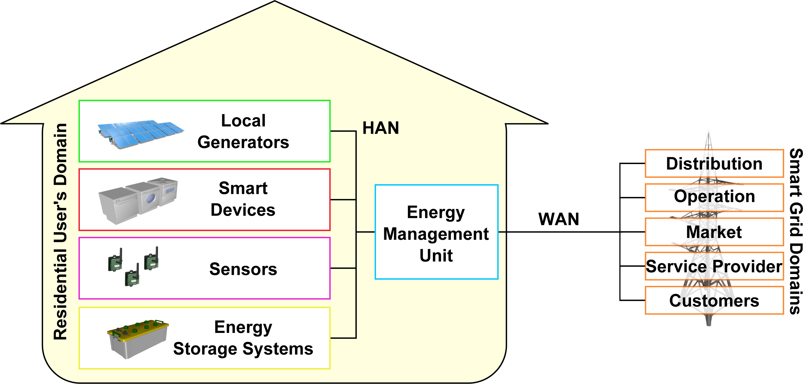
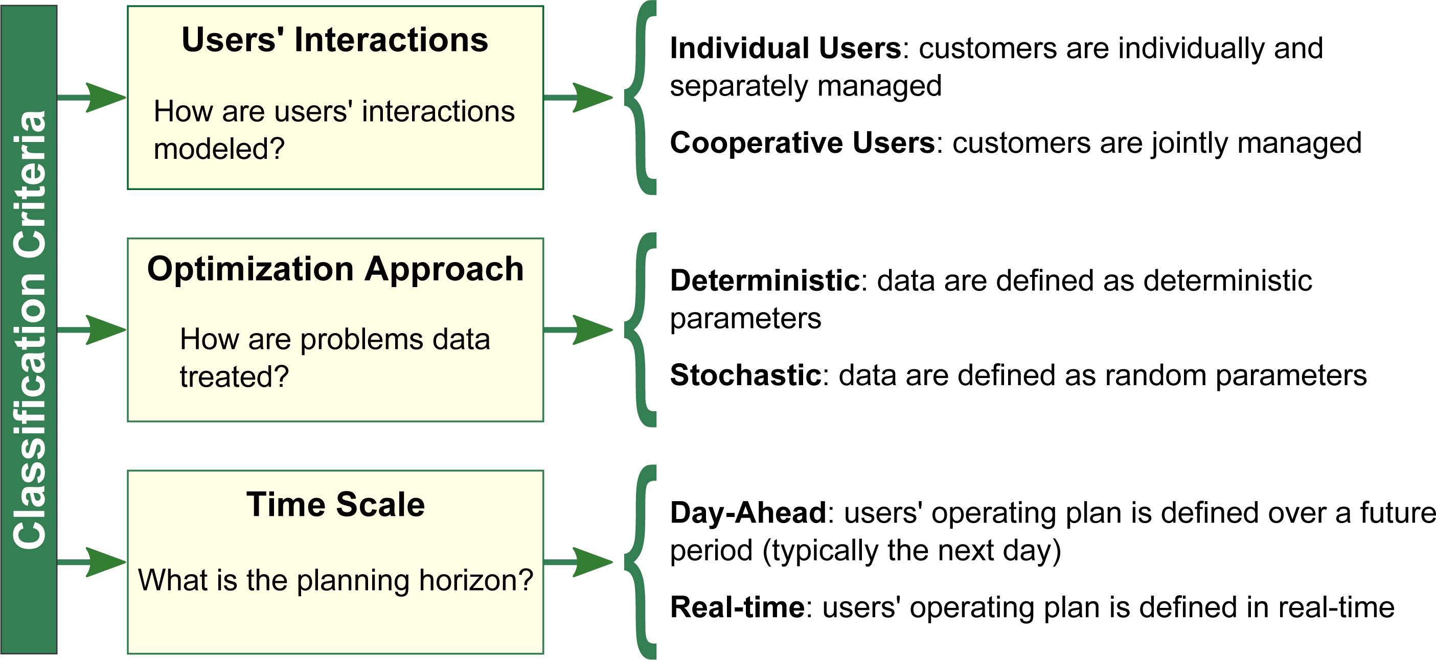
| Acronym | Definition |
|---|---|
| CPP | critical-peak pricing |
| DSM | demand-side management |
| EMU | energy management unit |
| ESS | energy storage system |
| HAN | home area network |
| HVAC | heating, ventilation and air conditioning |
| ISO | independent system operator |
| PEV | plug-in electric vehicle |
| PPD | peak power demand |
| PV | photovoltaic |
| RES | renewable energy source |
| RTP | real-time pricing |
| SOC | state of charge |
| TOU | time of use |
| WAN | wide area network |
| Sets | |
| Set of storage systems | |
| CB,HV AC | Set of HVAC devices |
| CB, EB | Set of comfort-based and energy-based elastic devices |
| , , | Sets of fixed, shiftable and elastic devices |
| Set of time slots | |
| Set of time slots within which the energy-based device e ∈ EB can be used | |
| Set of time slots within which the shiftable device s ∈ can be used | |
| Parameters | |
| ηC, ηD | Charging and discharging efficiencies of battery b ∈ [p.u.] |
| µ | Energy conversion parameter [h] |
| Maximum allowed power demand at time n ∈ [kW h] | |
| Energy generated by local RESs at time n ∈ [kW h] | |
| Duration of load profile of shiftable device s ∈ in terms of time slots [p.u.] | |
| Energy requirement of energy-based device e ∈ EB [kW h] | |
| Dissatisfaction for starting shiftable device s ∈ at time n ∈ [p.u.] | |
| Power consumption of shiftable device s ∈ in the d-th time slot of its load profile [kW ] | |
| , | Minimum and maximum power consumption of energy-based device e ∈ EB at time n ∈ [kW] |
| Power consumption of fixed device f ∈ at time n ∈ [kW] | |
| , | Maximum charging and discharging rates of battery b ∈ [kW] |
| Rewards paid at time n ∈ by the retailer if its demand increase/reduction requests are met [€] | |
| , | Minimum and maximum state of charge of battery b ∈ [kWh] |
| Minimum starting-time slot and maximum ending-time slot of energy-based device e ∈ EB [p.u.] | |
| Minimum starting-time slot and maximum ending-time slot of shiftable device s ∈ [p.u.] | |
| Outdoor temperature at time n ∈ [°C] | |
| Minimum and maximum power demand allowed by the retailer at time n ∈ [kW] | |
| Variables | |
| Net generation of RESs at time n ∈ [kW] | |
| Binary variables equal to one if the demand increase/reduction request of retailer at time n ∈ is satisfied [p.u.] | |
| cn, dn | Cost of energy bought and injected into the grid at time n ∈ [€/kW h] |
| Dissatisfaction of users for comfort-based device e ∈ CB at time n ∈ [p.u.] | |
| hn | Binary variable equal to one if at time n ∈ the user is injecting energy into the grid and zero otherwise [p.u.] |
| Power consumption of elastic device e ∈ at time n ∈ [kW ] | |
| Power consumption of comfort-based device e ∈ CB at time n ∈ [kW] | |
| Power consumption of energy-based device e ∈ EB at time n ∈ [kW] | |
| Overall power consumption of devices at time n ∈ [kW] | |
| Power consumption of shiftable device s ∈ at time n ∈ [kW ] | |
| Thermal comfort at time n ∈ [p.u.] | |
| Charging and discharging rates of battery b ∈ at time n ∈ [kW] | |
| SOCbn | State of charge of battery b ∈ in the time slot n ∈ [kW h] |
| Indoor temperature at time n ∈ [°C] | |
| wbn | Binary variable equal to one if battery b ∈ is charging at time n ∈ , and zero otherwise [p.u.] |
| Binary variable equal to one if shiftable device s ∈ starts at time n ∈ , and zero otherwise [p.u.] | |
| yn, zn | Energy bought and injected into the grid at time n ∈ [kWh] |
| Main Features | ||
|---|---|---|
| Users’ Interactions | Individual Users |
|
| Cooperative Users |
| |
| Optimization Approach | Deterministic |
|
| Stochastic |
| |
| Time Scale | Day-ahead |
|
| Real-time |
| |
© 2014 by the authors; licensee MDPI, Basel, Switzerland This article is an open access article distributed under the terms and conditions of the Creative Commons Attribution license (http://creativecommons.org/licenses/by/3.0/).
Share and Cite
Barbato, A.; Capone, A. Optimization Models and Methods for Demand-Side Management of Residential Users: A Survey. Energies 2014, 7, 5787-5824. https://doi.org/10.3390/en7095787
Barbato A, Capone A. Optimization Models and Methods for Demand-Side Management of Residential Users: A Survey. Energies. 2014; 7(9):5787-5824. https://doi.org/10.3390/en7095787
Chicago/Turabian StyleBarbato, Antimo, and Antonio Capone. 2014. "Optimization Models and Methods for Demand-Side Management of Residential Users: A Survey" Energies 7, no. 9: 5787-5824. https://doi.org/10.3390/en7095787