Fault Diagnosis and Fault-Tolerant Control of Wind Turbines via a Discrete Time Controller with a Disturbance Compensator

Abstract

This paper develops a fault diagnosis (FD) and fault-tolerant control (FTC) of pitch actuators in wind turbines. This is accomplished by combining a disturbance compensator with a controller, both of which are formulated in the discrete time domain. The disturbance compensator has a dual purpose: to estimate the actuator fault (which is used by the FD algorithm) and to design the discrete time controller to obtain an FTC. That is, the pitch actuator faults are estimated, and then, the pitch control laws are appropriately modified to achieve an FTC with a comparable behavior to the fault-free case. The performance of the FD and FTC schemes is tested in simulations with the aero-elastic code FAST.

1. Introduction

The feasibility of high value structures, such as wind turbines (WTs), depends, among other factors, on the costs associated with maintenance. Thus, research into methods of fault detection and isolation (FDI), as well as fault tolerant control (FTC) techniques that allow WTs to continue operating in the presence of faults (at least during a reasonable time to take a corrective action if the fault is severe and correctly detected) are the crux of the matter, as they will extend operating periods and, thus, minimize downtime and maximize the productivity of WTs [1,2]. The past few years have seen a rapid growth in interest in wind turbine FDI and FTC. For instance, [3] and [4] provide overviews of the recent status and practical aspects of these two research fields applied to WTs.

FDI techniques (also called fault diagnosis) can be classified into two categories: signal processing based and model based [5]. In the latter case, which is the approach used in this work, it is typical that a fault is said to be detected based on a residual signal. It must be a signal that is close to zero in the absence of a fault and significantly affected in the presence of faults [6]. The main components of a fault detection system are the following [6]: residual generator signal, residual evaluation method and prescribed threshold to decide whether a fault occurs or not [6]. It is then the task of fault isolation to categorize the type of fault and its location. Recently, there has been much interest in FDI in WTs. For example, observer-based schemes are provided in [7]. Support vector machine-based schemes are used in [8]. An automated fault detection and isolation scheme design method is presented in [9]. The work in [10] is based on parity equations. Data-driven methods are used in [11]. Finally, [12] is based on a generalized likelihood ratio method.

In control systems for wind turbines, robustness and fault tolerance capabilities are important properties, which should be considered in the design process, calling for a generic and powerful tool to manage parameter variations and model uncertainties [13]. In this paper, an active FTC is provided that is capable of handling the parameter variations along the nominal operating point and robust to the faults in the pitch system. In passive FTC systems, controllers are predetermined and are designed to be robust against a class of presumed faults. This approach needs neither FDI schemes nor controller reconfiguration, but it has limited fault-tolerant capabilities. In contrast, active FTC reacts to the system component failures actively by reconfiguring control actions so that the stability and acceptable performance of the entire system can be maintained [14]. A successful active FTC design relies heavily on real-time FDI schemes to provide the most up-to-date information about the true status of the system [14]. The main goal in this work is to design a controller with a suitable structure to achieve stability and satisfactory performance, not only when all control components are functioning normally, but also in case of (tolerable) faults. While still being a relatively new research topic, recent years have seen a growing number of publications in wind turbine FTC. For example, a set value-based observer method is proposed in [15], and [16] proposes a control allocation method for FTC of the pitch actuators. A virtual sensor/actuator scheme is applied in [17]. Takagi–Sugeno fuzzy-based methods for FTC for operation below rated wind speed are presented in [18]. The work in [19] presents an active FTC scheme based on adaptive methods, and a model predictive control scheme is used for FTC in [20].

In terms of control, the wind turbine works in two distinct regions. One is below the rated wind speed, in the partial load region, where the turbine is controlled to maximize the power capture. This is achieved by adjusting the generator torque to obtain an optimum ratio between the tip speed of the blades and the wind speed. The other one is above the rated wind speed, in the full load region, where the main task of the controller is to adapt the aerodynamic efficiency of the rotor by pitching the blades into or out of the wind to keep the rotor speed at its rated value. Blade control pitching is activated only in the full load region, while in the partial load region, the blades are kept by the controller at zero pitch angle [21]. Note that the switching of control between these two regions is gradual, normally using a so-called transition zone. In this paper, operation in the full load region, where the blade pitch control is acting, is considered.

Nowadays, pitch actuators are basically divided into two types: electric and hydraulic. Hydraulic actuators change the blade pitch angle through a hydraulic system. The method offers rapid response frequency, large torque, convenient centralization and is widely applied in WTs [22]. However, hydraulic systems may suffer from oil leakage, high air content in the oil, pump wear and pressure drop [2]. These faults are studied in this paper. In fact, the pitch actuators have the highest failure rate in WTs [2]. Thus, WT pitch sensors and actuators are often the topic of the FDI and FTC research focus. For example, an H-infinity-based FDI technique to detect and estimate the magnitude of blade bending moment sensor and pitch actuator faults is given in [23]; blade root bending measurements are used to detect pitch misalignment in [24]; model-based and system identification techniques are used for pitch actuator faults in [25]; a technique for detecting additive and multiplicative actuator faults is developed in [26]; FTC in the case of faulty blade load measurements is implemented in [27].

The main contribution of this paper is two-fold. First, a controller based on a disturbance compensator is proposed to face tolerable faults. Second, a fault-diagnosis algorithm is developed. The disturbance compensator and the controller are both formulated in the discrete time domain using the variable structure concept [28]. The actuator faults are estimated from the disturbance compensator, and the control inputs are then modified (with the estimated fault signal) to achieve fault-tolerant control in the presence of pitch actuator faults. The proposed techniques are validated using the aeroelastic wind turbine simulator software, FAST [29]. This simulator is designed by the U.S. National Renewable Energy Laboratory’s (NREL) National Wind Technology Center and widely used for studying wind turbine control systems. Since FAST is used by wind turbine researchers around the world, results based on this platform are more likely to be used by the wind industry than those based on a simpler model.

This paper is organized as follows. In Section 2, the onshore reference WT used in the simulations is introduced. In Section 4, the baseline control strategy, which will be used for comparison, is recalled. In Section 5, the control and disturbance estimation techniques are stated. The simulation results are presented in Section 6. Finally, Section 7 provides the conclusions.

2. Reference WT

Several FAST models of real and composite wind turbines of varying sizes are available in the public domain. In this work, the onshore version of a large WT that is representative of real utility-scale land- and sea-based multi-megawatt turbines described by [30] is used. This WT is a conventional three-bladed upwind variable-speed variable pitch-controlled turbine. In fact, it is a fictitious 5-MW machine with its properties based on a collection of existing wind turbines of similar rating, since not all turbine properties are published by manufacturers. The main properties of this turbine are listed in Table 1. This work deals with the full load region of operation: that is, the proposed controller’s main objective is that the electric power follows the rated power.

Table 1. Gross properties of the wind turbine [30].

Reference Wind Turbine
Rated power	5 MW
Number of blades	3
Rotor/hub diameter	126 m, 3 m
Hub height	90 m
Cut-in, rated, cut-out wind speed	3 m/s, 11.4 m/s, 25 m/s
Rated generator speed (ωng)	1, 173.7 rpm
Gearbox ratio	97

Table 1. Gross properties of the wind turbine [30].

Reference Wind Turbine
Rated power	5 MW
Number of blades	3
Rotor/hub diameter	126 m, 3 m
Hub height	90 m
Cut-in, rated, cut-out wind speed	3 m/s, 11.4 m/s, 25 m/s
Rated generator speed (ωng)	1, 173.7 rpm
Gearbox ratio	97

Here, the generator-converter and the pitch actuators are modeled and implemented externally; i.e., apart from the embedded FAST code. The next subsections present these models, as well as the wind model used in the simulations.

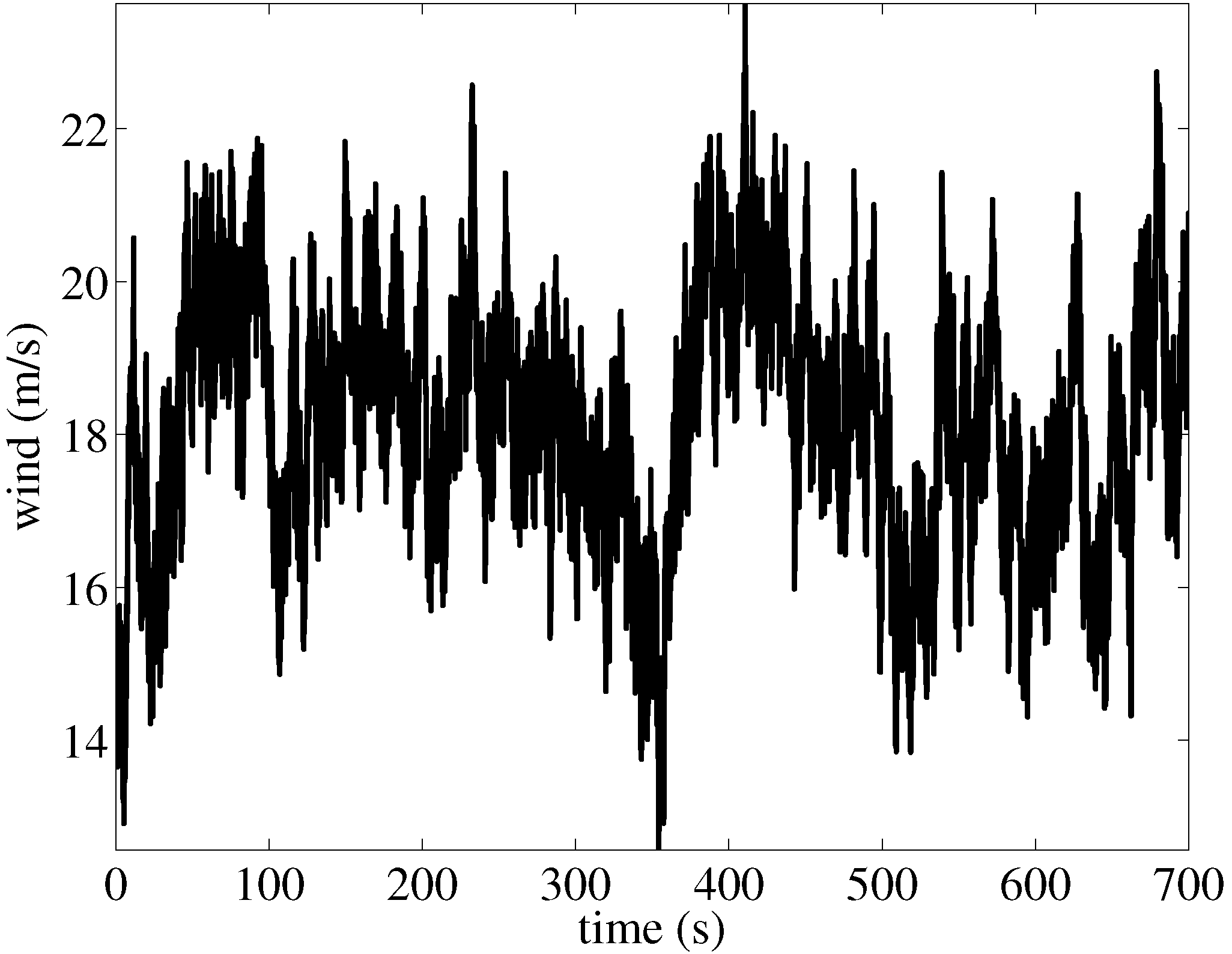
3. Wind Modeling

In fluid dynamics, turbulence is a flow regime characterized by chaotic property changes. This includes low momentum diffusion, high momentum convection and rapid variation of pressure and velocity in space and time. In the simulations, new wind datasets are generated in order to capture a more realistic turbulent wind simulation and, thus, to test the turbine controllers in a more realistic scenario. The turbulent-wind simulator TurbSim [31] developed by NRELis used. TurbSim generates a rectangular grid, which holds the wind data. The generated wind data have the following characteristics:

• Grid settings and position matched with the rotor diameter and the center of the grid positioned at hub height. This represents a grid size of 130 × 130 m centered at 19.55 m.
• The Kaimal turbulence model is selected.
• The turbulence intensity is set to 10%.
• Normal wind type is chosen with a logarithmic profile.
• Reference height is set to 90.25 m. This is the height where the mean wind speed is simulated.
• Mean (total) wind speed is set to 18.2 m/s.
• The roughness factor is set to 0.01 m, which corresponds to a terrain type of open country without significant buildings and vegetation.

It can be seen from Figure 1 that the wind speed covers the full load region, as its values range from 12.91 m/s up to the maximum of 22.57 m/s.

Figure 1. Hub-height wind speed for simulation tests. It is noteworthy that the simulated wind gust is from 350 to 400 s (approximately) where wind speed moves from 12.91 m/s up to the maximum of 22.57 m/s, followed by an abrupt decrease in the next 100 s.

Figure 1. Hub-height wind speed for simulation tests. It is noteworthy that the simulated wind gust is from 350 to 400 s (approximately) where wind speed moves from 12.91 m/s up to the maximum of 22.57 m/s, followed by an abrupt decrease in the next 100 s.

3.1. Generator-Converter Actuator Model

The dynamics of the generator-converter can be modeled by a first-order differential system [1], which is given by:

$${\dot{\text{τ}}}_r(t)+{\alpha }_{gc}{\text{τ}}_r(t)={\alpha }_{gc}{\text{τ}}_c(t)$$

where τ_r and τ_c are the real generator torque and its reference (given by the controller), respectively, where we set α_gc = 50 [30]. Additionally, the power produced by the generator, P_g(t), can be modeled using [1]:

$$P_g(t)={\eta }_g{\omega }_g(t){\text{τ}}_r(t)$$

where η_g is the efficiency of the generator and ω_g is the generator speed. In the numerical experiments, η_g = 0.98 is used [1].

3.2. Pitch Actuator Model

The hydraulic pitch system consists of three identical pitch actuators, which are modeled as a linear differential equation with time-dependent variables, pitch angle β(t) and its reference u(t). In principle, it is a piston servo-system, which can be expressed as a second-order differential system [1]:

$$\ddot{\text{β}}(t)+2\text{ξ}{\omega }_n\dot{\text{β}}(t)+{\omega }_n^2\text{β}(t)={\omega }_n^{2}u(t)$$

(1)

where ω_n and ξ are the natural frequency and the damping ratio, respectively. For the fault-free case, the parameters ξ = 0.6 and ω_n = 11.11 rad/s are utilized. [1].

3.3. Fault Description

Faults in a WT have different degrees of severity and accommodation requirements. A safe and fast shutdown of the WT is necessary for some of them, while for others, the system can be reconfigured to continue electrical power generation. Variable structure controllers can be applied in the case of failures that gradually change the system’s dynamics. In this work, pitch actuator faults are studied as they are the actuators with the highest failure rate in WTs [2]. A fault may change the dynamics of the pitch system by varying the damping ratio and the natural frequencies from their nominal values to their faulty values in Equation (1). The parameters for the pitch system under different conditions are given in Table 2. The normal air content in the hydraulic oil is 7%, whereas the high air content in the oil fault (F1) corresponds to 15%. Pump wear (F2) represents the situation of 75% pressure in the pitch system, while the parameters stated for hydraulic leakage (F3) correspond to a pressure of only 50%.

Table 2. Parameters for the hydraulic pitch system under different conditions [2].

Faults	ωn (Rad/s)	ξ
Fault-free (FF)	11.11	0.6
High air content in oil (F1)	5.73	0.45
Pump wear (F2)	7.27	0.75
Hydraulic leakage (F3)	3.42	0.9

Table 2. Parameters for the hydraulic pitch system under different conditions [2].

Faults	ωn (Rad/s)	ξ
Fault-free (FF)	11.11	0.6
High air content in oil (F1)	5.73	0.45
Pump wear (F2)	7.27	0.75
Hydraulic leakage (F3)	3.42	0.9

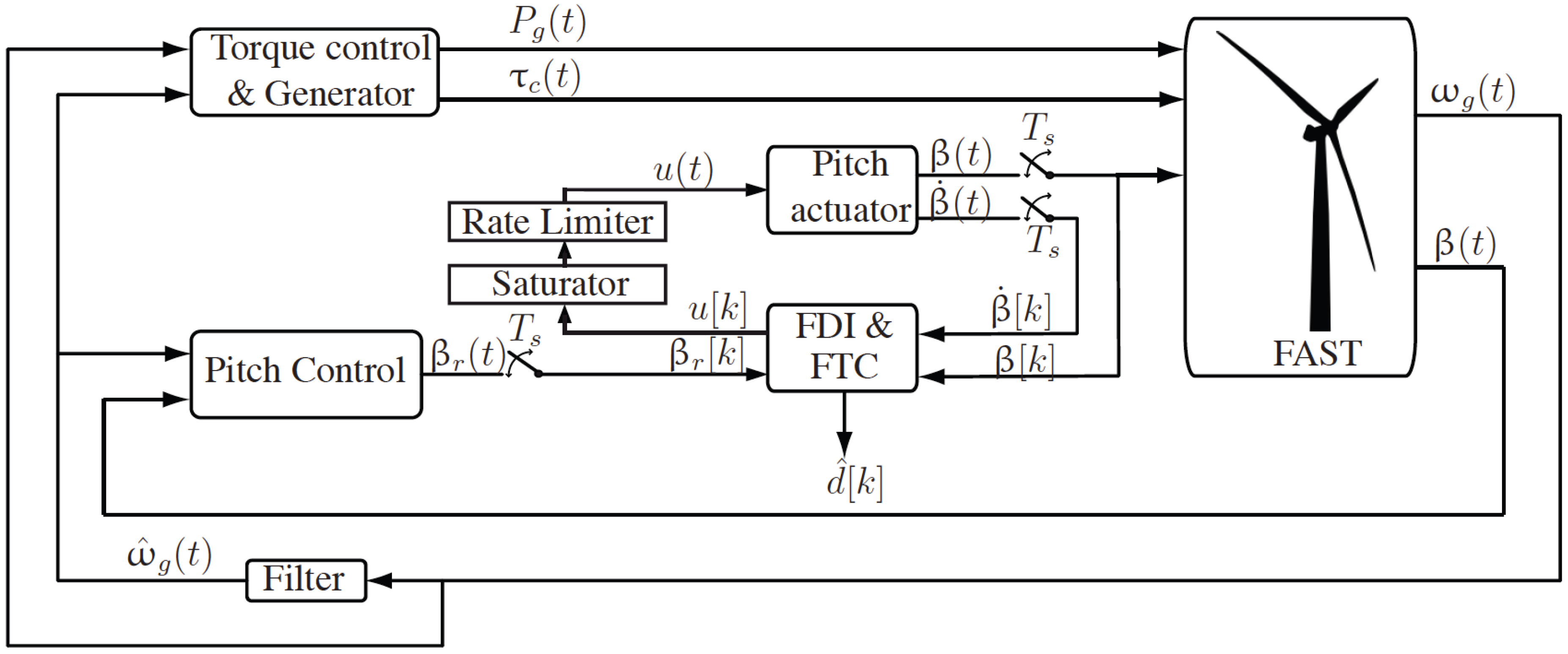
4. Baseline Control Strategy

The three-bladed 5-MW reference WT given by FAST contains a torque and pitch controllers for the full load region; see [30]. In this section, we recall these controllers and refer to them as the baseline torque, and pitch controllers as their performance in the fault-free scenario will be used for comparison with the proposed FTC technique stated in Section 5.

Both the torque control and the pitch control will use the generator speed measurement as the input. To mitigate high-frequency excitation of the control systems, we filtered the generator speed measurement for both the torque and pitch controllers using a recursive, single-pole low-pass filter with exponential smoothing, as proposed in [30].

In the full load region, the torque controller maintains constant the generator power; thus, the generator torque is inversely proportional to the filtered generator speed or,

$${\text{τ}}_c(t)=\frac{P_{\text{ref}}}{{\widehat{\omega }}_g(t)}$$

(2)

where P_ref is the reference power and ${\widehat{\omega }}_g$ is the filtered generator speed. This controller will be referred to as the baseline torque controller. As the generator may not be able to supply the desired electromechanic torque depending on the operating conditions and in the case of overshooting, the torque controller is saturated to a maximum of 47, 402.9 Nm and a maximum rate limit of 15, 000 Nm/s; see [30].

To assist the torque controller with regulating the WT electric power output, while avoiding significant loads and maintaining the rotor speed within acceptable limits, a collective pitch controller is added to the rotor speed tracking error. The collective blade pitch gain scheduling PI-controller (GSPI) is one of the first well-documented controllers, and it is used in the literature as a baseline controller to compare the obtained results [2]. This work will follow the same steps and use the baseline GSPI controller to study the blade pitching system in the fault-free scenario. The GSPI is a collective pitch controller that employs a gain-scheduling technique to compensate for the nonlinearity in the turbine by changing the controller gain according to a scheduling parameter. This controller was originally developed by Jonkman for the standard land-based 5-MW turbine [30]. The GSPI control has the generator speed as the input and the pitch servo set-point, β_r(t), as the output. That is,

$$\begin{array}{cc}{\text{β}}_r(t)=K_p(\text{θ})\left({\widehat{\text{ω}}}_g(t)-{\text{ω}}_{ng}\right)+K_i(\text{θ}){\displaystyle {\int }_0^t\left({\widehat{\text{ω}}}_g(\text{τ})-{\text{ω}}_{ng}\right)d\text{τ}},& K_p>0, K_i>0\end{array}$$

(3)

where ${\widehat{\omega }}_g(t)$ is the filtered generator speed, ω_ng is the nominal generator speed (at which the rated electrical power of the WT is obtained) and the scheduling parameter θ is taken to be the previously measured collective blade pitch angle. As the three pitch angles are measured, the collective pitch angle is obtained by averaging the measurements of all pitch angles. The scheduled gains are calculated following [30]. Finally, a pitch limit saturation to a maximum of 45° and a pitch rate saturation of 8°/s are implemented; see [30].

5. Fault-Tolerant Control

This section details the design of the FTC strategy based on a control plus disturbance estimator in the time discrete domain. The control objective is the tracking of the reference signal β_r(t) (given by the baseline pitch controller; see Equation (3)) and its corresponding velocity, even in the case of pitch actuator fault. The block diagram in Figure 2 shows the connections between the WT (simulated using FAST), the FTC system, the pitch actuator and the torque and pitch controllers. To discretize continuous signals, a conventional sampler is used. As can be seen in the block diagram in Figure 2, a switch closes to admit an input signal every sampling period T_s. The sampler converts the continuous time signal into a train of pulses occurring at the sampling instants kT_s for k = 0, 1, 2, .... Traditionally, a discrete time signal is considered to be undefined at points in time between the sample times. In this work, discrete time signals remain defined between sample times by holding the value at the previous sample time. That is, when the value of a discrete signal is measured between sample times, the value of the signal at the previous sample time is observed. This is known as a zero-order hold or the staircase generator, as the output of a zero-order hold is a staircase function. In this paper, the notation [k] is used for these discrete time signals.

Taking the pitch actuator system given in Equation (1), the state space representation in discrete time, using Euler approximation, leads to:

$$x\left[k+1\right]=\left(A+\Delta A\right)x[k]+bu[k]=Ax[k]+\Delta Ax[k]+bu[k]$$

(4)

where:

$$x\left[k+1\right]=\left(\begin{array}{c}\text{β}\left[k+1\right]\\ \dot{\text{β}}\left[k+1\right]\end{array}\right), A=\left(\begin{array}{cc}1& T_s\\ -{\text{ω}}_n^2{T}_s& 1-2\xi {\text{ω}}_n{T}_s\end{array}\right), x[k]=\left(\begin{array}{c}\text{β}\left[k\right]\\ \dot{\text{β}}\left[k\right]\end{array}\right), b=\left(\begin{array}{c}0\\ T_s{\text{ω}}_n^2\end{array}\right)$$

(5)

where ∆A accounts for a fault in the system, and thus, ∆Ax[k] is a disturbance term that will be estimated.

Figure 2. Block diagram of the closed loop system. Note that the torque control and the pitch control already include their respective saturator and rate limiter blocks.

Figure 2. Block diagram of the closed loop system. Note that the torque control and the pitch control already include their respective saturator and rate limiter blocks.

In order to design the control law u[k], the control objective is that, even in a faulty case, the real pitch angle β follows the commanded reference pitch angle β_r (given by the pitch controller), as well as the velocity $\dot{\text{β}}$ follows the commanded reference ${\dot{\text{β}}}_r$. That is, the objective is to ensure the asymptotic convergence of the tracking error vector to zero. The error vector is defined as:

$$e\left[k\right]={(e_1[k], e_2[k])}^T={(\text{β}[k]-{\text{β}}_r[k], \dot{\text{β}}[k]-{\dot{\text{β}}}_r[k])}^T$$

Following the results in [28], the switching function is defined with the error vector and a column vector c as follows:

$$s[k]=c^{T}e[k],$$

(6)

and then, for System 4-5, the sliding surface 6 gives the asymptotic convergence of the tracking error vector to zero designing vector c, such that the matrix:

$$\left[I-b{\left(c^{T}b\right)}^{-1}{c}^T\right] A$$

(7)

is contractive (eigenvalues inside the unit circle). When using a sample time T_s = 0.0125 (see [30]) and the fault-free values for the parameters ω_n and ξ, it is found that vector:

$$c={(1, 0.25)}^T$$

ensures that Matrix 7 is contractive (with one eigenvalue equal to zero as in the application example given by [28]). Finally, to achieve the sliding mode, a new control law with a disturbance estimation law is proposed [28], as follows:

$$u[k]=-\widehat{d}[k]+{\left(c^{T}b\right)}^{-1}\left[c^T\left(\begin{array}{c}{\text{β}}_r\left[k\right]\\ {\dot{\text{β}}}_r\left[k\right]\end{array}\right)-c^{T}Ax[k]+qs[k]-\eta \text{sgn}(s[k])\right]$$

(8)

$$\widehat{d}[k]=\widehat{d}[k-1]+{\left(c^{T}b\right)}^{-1}g[s[k]-qs[k-1]+\eta \text{sgn}(s[k-1])]$$

(9)

where 0 ≤ q ≤ 1, 0 < g < 1 and η > 0 and $\widehat{d}[k]$ being the fault estimator or also called the disturbance estimator. In the numerical simulations: q = g = 1/2 and η = 100. As can be seen in Equation (8), the proposed discrete controller for active FTC is dependent on a fault estimate, $\widehat{d}[k]$, provided by the fault diagnosis system. Note that [28] contributes a disturbance compensator and controller for regulation or tracking purposes only. The novelty of the present work is to extend the work in [28] by its inclusion in a new fault-tolerant control scheme and fault detection system (see the block diagram in Figure 2). The design of a continuous residual signal capable of isolating the type of fault (among the studied faults F1, F2 and F3) is also a contribution of this paper (see Figure 3 and Figure 4).

The pitch controller used by the FTC strategy is the baseline GSPI controller; see Section 4. On the other hand, the used torque controller is the chattering control proposed in [32], which is recalled here to be:

$${\dot{\text{τ}}}_c(t)=\frac{-1}{{\widehat{\text{ω}}}_g(t)}\left[{\text{τ}}_c(t)(a{\widehat{\text{ω}}}_g(t)+{\dot{\widehat{\text{ω}}}}_g(t))-a{P}_{\text{ref}}+K_{\alpha }\text{sgn}(P_{\text{e}}(t)-P_{\text{ref}})\right]$$

(10)

where P_ref is the reference power and P_e is the electrical power, considered here (only for the control design) to be described as [33]:

$$P_{\text{e}}(t)={\text{τ}}_c(t){\widehat{\text{ω}}}_g(t)$$

(11)

where τ_c(t) is the torque control and ${\widehat{\text{ω}}}_g(t)$ is the filtered generator speed. This chattering controller (Equation (10)) has several advantages (see [32]):

• It ensures that the closed-loop system has finite time stability of the equilibrium point (P_e(t)−P_ref), and the settling time can be chosen by properly defining the values of the parameters a and K_α.
• It does not require information from the turbine total external damping or the turbine total inertia. It only requires the filtered generator speed and reference power of the WT.

In the numerical simulations, the values a = 1 and K_α = 1.5 × 10⁵ have been used, and a first order approximation of ${\dot{\widehat{\text{ω}}}}_g(t)$ is computed.

This torque controller is saturated to a maximum of 47, 402.91 Nm and a maximum generator torque rate saturation of 15, 000 Nm/s, similarly to the baseline one.

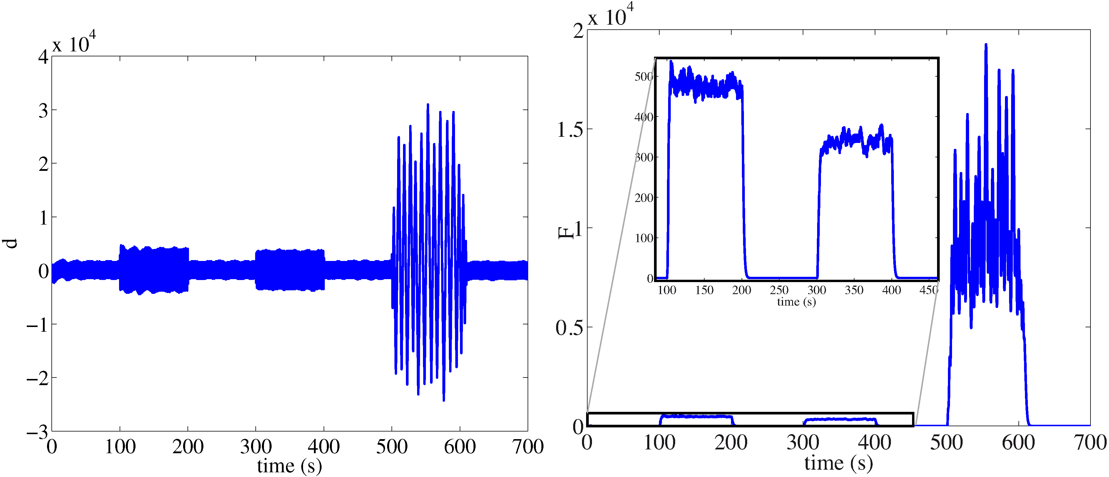
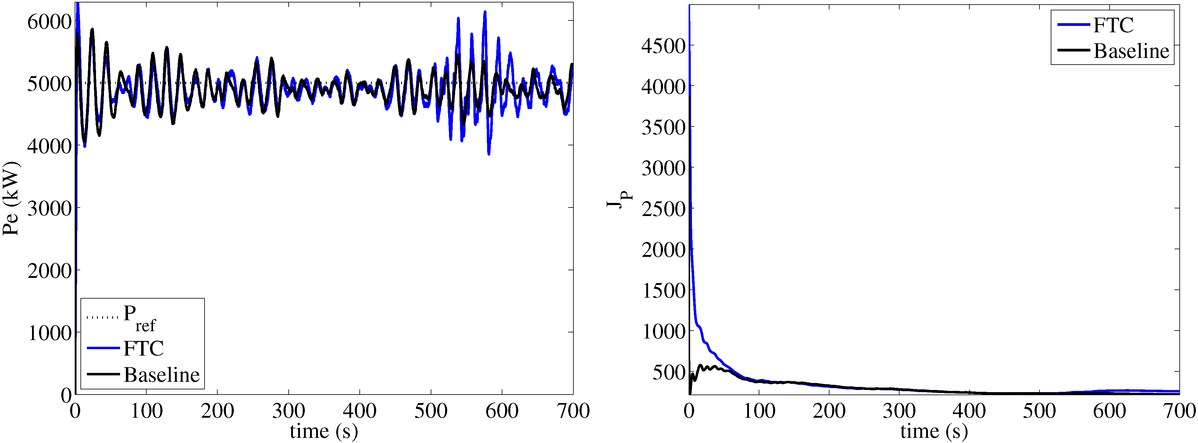
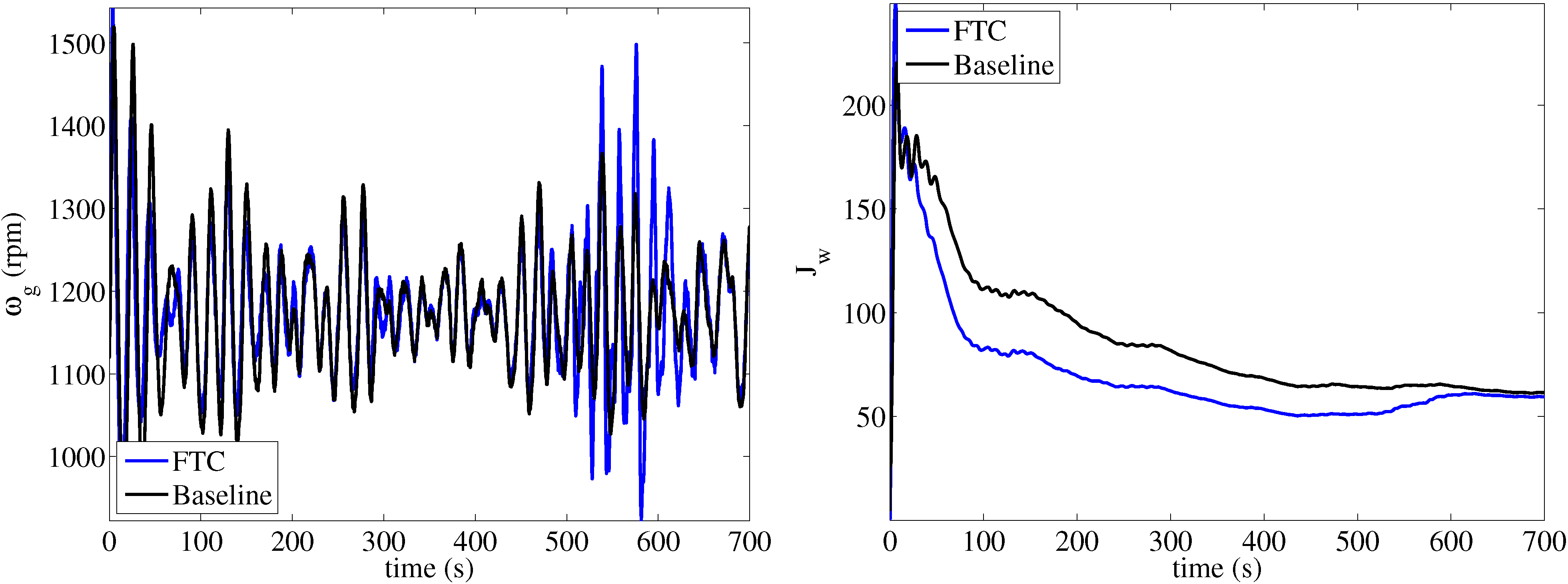
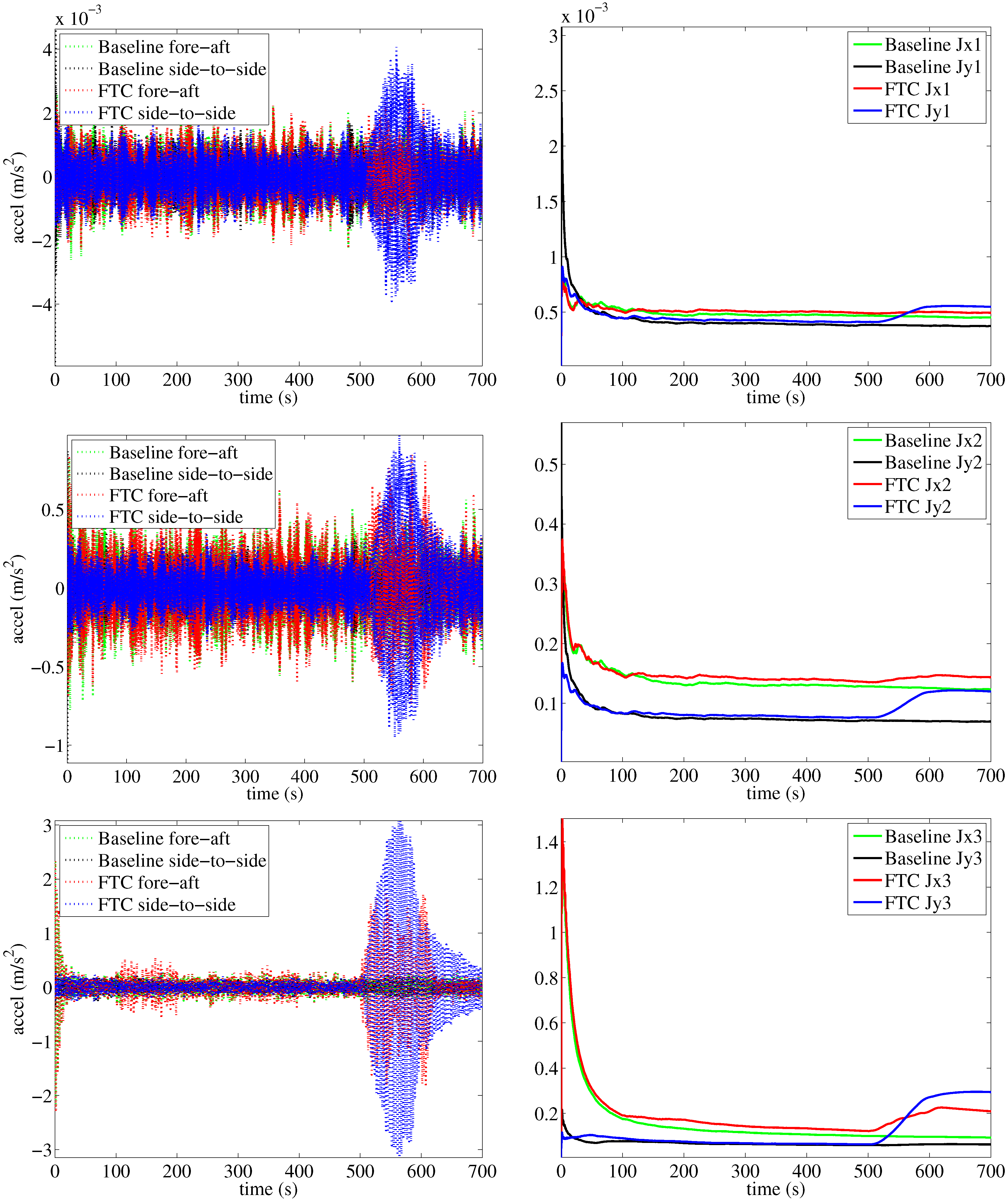
6. Results

The results compare the performance of the contributed FTC technique under different faulty scenarios with respect to the fault-free case with the baseline torque controller. When testing the FTC technique, the faults given in Table 2 are introduced only in the third pitch actuator (thus, β₁ and β₂ are always fault-free) in the following way:

• From 0 to 100 s, it is fault-free.
• From 100 to 200 s, a fault due to high air content in the oil (F1) is active.
• From 200 to 300 s, it is fault-free.
• From 300 to 400 s, a fault due to pump wear (F2) is active.
• From 400 to 500 s, it is fault-free.
• From 500 to 600 s, a fault due to hydraulic leakage (F3) is active.
• From 600 to 700 s, it is fault-free.

The response of the generator velocity, electrical power and accelerations are analyzed in terms of the normalized integral absolute error through the following performance indices [34]:

$$\begin{array}{c}{J}_w(t)=\frac{1}{t}{\displaystyle {\int }_0^t|{\text{ω}}_g(\text{τ})-{\text{ω}}_{ng}|d\text{τ}}\\ J_P(t)=\frac{1}{t}{\displaystyle {\int }_0^t|P_g(\text{τ})-P_{\text{ref}}|d\text{τ}}\\ J_{xi}(t)=\frac{1}{t}{\displaystyle {\int }_0^t|a_{x,i}(\text{τ})|d\text{τ}}\hspace{1em}i=1, 2, 3\\ J_{yi}(t)=\frac{1}{t}{\displaystyle {\int }_0^t|a_{y,i}(\text{τ})|d\text{τ}}\hspace{1em}i=1, 2, 3\end{array}$$

Note that a_xi(t) are the fore-aft and a_yi(t) the side-to-side accelerations at nodes located at the tower bottom (i = 1), at mid-tower height (i = 2) and at the tower top (i = 3).

As can be seen in Figure 3 (left), the three types of faults are detected by the disturbance estimator $\widehat{d}$ given in Equation (9). To finally setup the fault detection and isolation strategy, the proposed residual signal, r(t), is computed as described in Figure 4, and its results are shown in Figure 3 (right). This residual is close to zero when the system is fault-free. On the other hand, when a fault appears, it is significantly affected and allows one to isolate the type of fault (among the three studied pitch actuator faults stated in Table 2). The used thresholds to pinpoint the type of fault are:

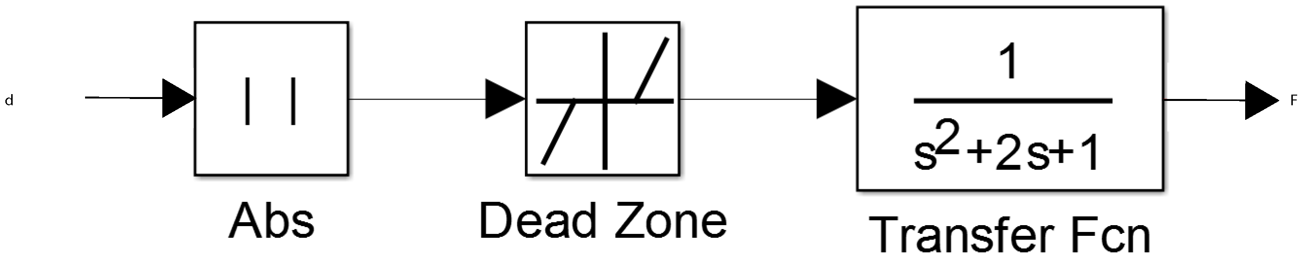
• When the signal is smaller than 400, then F2 is detected. This can be seen in the zoom in Figure 3 (right).
• When the signal is between 400 and 5000, then F1 is detected.
• When the signal is above 5000. then F3 is detected.

Figure 3. Discrete disturbance estimator (left) and the continuous residual signal (right).

Figure 3. Discrete disturbance estimator (left) and the continuous residual signal (right).

Figure 4. Computation of the residual signal, r(t). Note that the Simulink^® dead zone block is used (start of dead zone value equal to zero and end of dead zone value equal to 2000).

Figure 4. Computation of the residual signal, r(t). Note that the Simulink^® dead zone block is used (start of dead zone value equal to zero and end of dead zone value equal to 2000).

Note that in discrete time, the concept of the sliding mode surface is in fact a quasi-sliding mode (see, for instance, [35]). That is the reason in Figure 5 (left) that the typical finite time convergence, given by continuous slide-mode controllers, is not obtained here. In the discrete case, the typical convergence consists of the values of the trajectory being maintained inside an interval, as can be seen in Figure 5 (left).

Figure 5. Electrical power (left) and J_P index (right).

Figure 5. Electrical power (left) and J_P index (right).

It can be seen from Figure 5 and Figure 6 that the system behavior (electrical power and generator speed) with active fault compensation is similar to the behavior of the fault-free case, as the performance indices’, J_P(t) and J_w(t), values for the fault-free baseline and for the FTC (with faults) are very close. Moreover, the J_w(t) performance index shows that the generator speed is closer to the nominal one during faults F1 and F2 for the FTC than for the (fault-free) baseline controller. This can be seen in Figure 6 (right), as the values of the index, during faults F1 and F2, are smaller for the FTC strategy.

Figure 6. Generator speed (left) and J_w index (right).

Figure 6. Generator speed (left) and J_w index (right).

Figure 7 (left) shows that the first pitch angle (β₁), which is always fault-free, has a slightly different behavior with the FTC than with the baseline control. This is due to the fact that with the FTC technique, a fault is introduced in the third pitch actuator (β₃), as can be seen in Figure 7 (right). Although higher oscillations are present in the FTC, the pitch control signal is regulated within the authorized variation domain. That is, none of the variations exceed the mechanical limitations of the pitch actuator.

Figure 7. First pitch angle (left) and third pitch angle (right).

Figure 7. First pitch angle (left) and third pitch angle (right).

As can be seen in Figure 8, the fore-aft and side-to-side accelerations are similar for the FTC technique (with faults) and for the fault-free baseline control strategy. The performance indices J_xi(t) and J_yi(t) at different tower heights corroborate this statement, as their values are similar for the FTC and the baseline control strategy.

On the other hand, it is well known that actuator saturation causes stability problems in control systems [36]. This problem might also appear in the proposed FTC technique when torque saturation and/or pitch actuator saturation occur. Note that, although it is out of the scope of this paper, the problem can be overpassed using, for instance, the well-known anti-windup technique (see [37]).

Figure 8. Fore-aft and side-to-side accelerations (left) and related indices (right) at nodes located at the tower bottom, at mid-tower height and at the tower top.

Figure 8. Fore-aft and side-to-side accelerations (left) and related indices (right) at nodes located at the tower bottom, at mid-tower height and at the tower top.

Finally, note that when a fault appears in a mechanical system, normally, this fault will worsen, especially if the system remains in operation. The evolution of the failure can result in a disaster. To be realistic with robustness to a mechanical failure, the fault modeling should capture its evolution when the system remains in operation (time-varying parameters, among other nonlinearities). The evolution of the faults is not modeled in this paper. Thus, the results of this paper guarantee the controller robustness for a reasonable time in order to take action and correct the fault.

7. Conclusions

A WT fault-tolerant control scheme for pitch actuator faults is presented in this paper based on direct fault estimation by means of a disturbance compensator. With the proposed FTC strategy, the system behavior in FAST simulations with faults is close to the behavior of the baseline controllers in the fault-free case. Meanwhile, the proposed residual signal detects in a short time the appearance of the faults. This is in itself a benefit for the development of fault diagnosis schemes for WT. Finally, note that the resulting FTC strategy can also be easily implemented in practice due to low data storage and simple math operations (at each sampling time, sums and products between scalars).

References

- Odgaard, P.; Johnson, K. Wind Turbine Fault Diagnosis and Fault Tolerant Control—An Enhanced Benchmark Challenge. In Proceedings of the 2013 American Control Conference—ACC, Washington, DC, USA, 17–19 June 2013; pp. 1–6.
- Chaaban, R.; Ginsberg, D.; Fritzen, C.P. Structural Load Analysis of Floating Wind Turbines Under Blade Pitch System Faults. In Wind Turbine Control and Monitoring; Luo, N., Vidal, Y., Acho, L., Eds.; Springer: Zürich, Switzerland, 2014; pp. 301–334. [Google Scholar]
- Amirat, Y.; Benbouzid, M.E.H.; Al-Ahmar, E.; Bensaker, B.; Turri, S. A brief status on condition monitoring and fault diagnosis in wind energy conversion systems. Renew. Sustain. Energy Rev. 2009, 13, 2629–2636. [Google Scholar] [CrossRef] [Green Version]
- Hameed, Z.; Ahn, S.; Cho, Y. Practical aspects of a condition monitoring system for a wind turbine with emphasis on its design, system architecture, testing and installation. Renew. Energy 2010, 35, 879–894. [Google Scholar] [CrossRef]
- Zeng, J.; Lu, D.; Zhao, Y.; Zhang, Z.; Qiao, W.; Gong, X. Wind turbine fault detection and isolation using support vector machine and a residual-based method. In Proceedings of the American Control Conference (ACC), Washington, DC, USA, 17–19 June 2013; pp. 3661–3666.
- Vidal, Y.; Acho, L.; Pozo, F. Robust fault detection in hysteretic base-isolation systems. Mech. Syst. Signal Process. 2012, 29, 447–456. [Google Scholar] [CrossRef]
- Chen, W.; Ding, S.X.; Sari, A.; Naik, A.; Khan, A.Q.; Yin, S. Observer-based fdi schemes for wind turbine benchmark. In Proceedings of the IFAC World Congress, Milano, Italy, 28 August–2 September 2011; pp. 7073–7078.
- Stoican, F.; Raduinea, C.F.; Olaru, S. Adaptation of set theoretic methods to the fault detection of wind turbine benchmark. In Proceedings of the IFAC World Congress, Milano, Italy, 28 August–2 September 2011; pp. 8322–8327.
- Svärd, C.; Nyberg, M. Automated design of an fdi-system for the wind turbine benchmark. In Proceedings of the IFAC World Congress, Milano, Italy, 28 August–2 September 2011; Volume 18, pp. 8307–8315.
- Pisu, P.; Ayalew, B. Robust fault diagnosis for a horizontal axis wind turbine. In Proceedings of the IFAC World Congress, Milano, Italy, 28 August–2 September 2011; Volume 2, pp. 7055–7060.
- Dong, J.; Verhaegen, M. Data driven fault detection and isolation of a wind turbine benchmark. In Proceedings of the IFAC World Congress, Milano, Italy, 28 August–2 September 2011; Volume 2, pp. 7086–7091.
- Kiasi, F.; Prakash, J.; Shah, S.; Lee, J.M. Fault detection and isolation of benchmark wind turbine using the likelihood ratio test. In Proceedings of the IFAC World Congress, Milano, Italy, 28 August–2 September 2011; pp. 7079–7085.
- Sloth, C.; Esbensen, T.; Stoustrup, J. Robust and fault-tolerant linear parameter-varying control of wind turbines. Mechatronics 2011, 21, 645–659. [Google Scholar] [CrossRef]
- Jiang, J.; Yu, X. Fault-tolerant control systems: A comparative study between active and passive approaches. Ann. Rev. Control 2012, 36, 60–72. [Google Scholar] [CrossRef]
- Casau, P.; Rosa, P.A.N.; Tabatabaeipour, S.M.; Silvestre, C. Fault detection and isolation and fault tolerant control of wind turbines using set-valued observers. In Proceedings of the 8th IFAC Symposium on Fault Detection, Supervision and Safety of Technical Processes, Mexico City, Mexico, 29–31 August 2012; pp. 120–125.
- Kim, J.; Yang, I.; Lee, D. Control allocation based compensation for faulty blade actuator of wind turbine. In Proceedings of the 8th IFAC Symposium on Fault Detection, Supervision and Safety of Technical Processes, Mexico City, Mexico, 29–31 August 2012; Volume 8, pp. 355–360.
- Rotondo, D.; Nejjari, F.; Puig, V.; Blesa, J. Fault tolerant control of the wind turbine benchmark using virtual sensors/actuators. In Proceedings of the 8th IFAC Symposium on Fault Detection, Supervision and Safety of Technical Processes, Mexico City, Mexico, 29–31 August 2012; Volume 8, pp. 114–119.
- Sami, M.; Patton, R.J. Global wind turbine FTC via TS fuzzy modelling and control. In Proceedings of the 8th IFAC Symposium on Fault Detection, Supervision and Safety of Technical Processes, Mexico City, Mexico, 29–31 August 2012; Volume 8, pp. 325–330.
- Simani, S.; Castaldi, P. Active actuator fault-tolerant control of a wind turbine benchmark model. Int. J. Robust Nonlinear Control 2014, 24, 1283–1303. [Google Scholar]
- Yang, X.; Maciejowski, J. Fault-tolerant model predictive control of a wind turbine benchmark. In proceedings of the 8th IFAC Symposium on Fault Detection, Supervision and Safety of Technical Processes, Mexico City, Mexico, 29–31 August 2012; pp. 337–342.
- Pao, L.Y.; Johnson, K.E. Control of wind turbines. IEEE Control Syst. 2011, 31, 44–62. [Google Scholar] [CrossRef]
- Zhao, W.; Qin, L.; Yao, X.; Shan, G. Modeling Research of MW Wind Turbine Variable Pitch System. Mach. Tool Hydraul. 2006, 6, 056. [Google Scholar]
- Wei, X.; Verhaegen, M.; van Engelen, T. Sensor fault detection and isolation for wind turbines based on subspace identification and Kalman filter techniques. Int. J. Adapt. Control Signal Process. 2010, 24, 687–707. [Google Scholar] [CrossRef]
- Dolan, B. Wind Turbine Modelling, Control and Fault Detection. Ph.D. Thesis, Technical University of Denmark, Lyngby, Denmark, August 2010. [Google Scholar]
- Donders, S.; Verdult, V.; Verhaegen, M. Fault Detection and Identification for Wind Turbine Systems: A Closed-Loop Analysis. Master’s Thesis, University of Twente, Enschede, The Netherlands, June 2002. [Google Scholar]
- Mešic, S.; Verdult, V.; Verhaegen, M.; Kanev, S. Estimation and robustness analysis of actuator faults based on Kalman filtering. In proceedings of the 5th IFAC Symposium on Fault Detection, Supervision and Safety of Technical Processes, Washington, DC, USA, 9–11 June 2003; pp. 241–246.
- Dobrila, C.; Stefansen, R. Fault Tolerant Wind Turbine Control. Master’s Thesis, Technical University of Denmark, Kgl. Lyngby, Denmark, 31 August 2007. [Google Scholar]
- Eun, Y.; Kim, J.H.; Kim, K.; Cho, D.I. Discrete-time variable structure controller with a decoupled disturbance compensator and its application to a CNC servomechanism. IEEE Trans. Control Syst. Technol. 1999, 7, 414–423. [Google Scholar]
- Jonkman, J. National Wind Technology Center Computer-Aided Engineering Tools (FAST). Available online: https://nwtc.nrel.gov/FAST (accessed on 7 May 2015).
- Jonkman, J.M.; Butterfield, S.; Musial, W.; Scott, G. Definition of a 5-MW Reference Wind Turbine for Offshore System Development; Technical Report; National Renewable Energy Laboratory: Golden, CO, USA, 2009. [Google Scholar]
- Kelley, N.; Jonkman, B. National Wind Technology Center Computer-Aided Engineering Tools (Turbsim), Last modified 30 May 2013. Available online: https://nwtc.nrel.gov/TurbSim (accessed on 7 May 2015).
- Vidal, Y.; Acho, L.; Luo, N.; Zapateiro, M.; Pozo, F. Power Control Design for Variable-Speed Wind Turbines. Energies 2012, 5, 3033–3050. [Google Scholar] [CrossRef]
- Boukhezzar, B.; Lupu, L.; Siguerdidjane, H.; Hand, M. Multivariable control strategy for variable speed, variable pitch wind turbines. Renew. Energy 2007, 32, 1273–1287. [Google Scholar] [CrossRef]
- Hofmann, J.; Dittmer, A. Model-based control of the flying helicopter simulator: Evaluating and optimizing the feedback controller. CEAS Aeronaut. J. 2011, 2, 43–56. [Google Scholar] [CrossRef]
- Gao, W.; Wang, Y.; Homaifa, A. Discrete-time variable structure control systems. IEEE Trans. Ind. Electron. 1995, 42, 117–122. [Google Scholar]
- Hu, T.; Lin, Z. Control Systems with Actuator Saturation: Analysis and Design; Springer Science & Business Media: Boston, MA, USA, 2001. [Google Scholar]
- Galeani, S.; Tarbouriech, S.; Turner, M.; Zaccarian, L. A tutorial on modern anti-windup design. Eur. J. Control 2009, 15, 418–440. [Google Scholar] [CrossRef]
© 2015 by the authors; licensee MDPI, Basel, Switzerland. This article is an open access article distributed under the terms and conditions of the Creative Commons Attribution license (http://creativecommons.org/licenses/by/4.0/).
Share and Cite
Vidal, Y.; Tutivén, C.; Rodellar, J.; Acho, L. Fault Diagnosis and Fault-Tolerant Control of Wind Turbines via a Discrete Time Controller with a Disturbance Compensator. Energies 2015, 8, 4300-4316. https://doi.org/10.3390/en8054300
Vidal Y, Tutivén C, Rodellar J, Acho L. Fault Diagnosis and Fault-Tolerant Control of Wind Turbines via a Discrete Time Controller with a Disturbance Compensator. Energies. 2015; 8(5):4300-4316. https://doi.org/10.3390/en8054300
Chicago/Turabian StyleVidal, Yolanda, Christian Tutivén, José Rodellar, and Leonardo Acho. 2015. "Fault Diagnosis and Fault-Tolerant Control of Wind Turbines via a Discrete Time Controller with a Disturbance Compensator" Energies 8, no. 5: 4300-4316. https://doi.org/10.3390/en8054300