1. Introduction
Electricity is becoming an integral part of life. It is a scare resource that needs to be utilized resourcefully. Peaks created due to electricity usage are not only disruptive for power grids but also cause high electricity bills. For a normal home whose electricity consumptions is doubled, line losses increase by a factor of four. A reduction of one kilowatt behaves differently if the upper bound and lower bound is different. Electric power cost savings by lessening consumption from 5 KW to 4 KW is much lower than reducing from 50 KW to 49 KW. Line losses make the major difference [
1]. Normalizing electricity consumption to avoid PC peaks is a vital solution for preserving electric power and ultimately reducing its cost.
With the advent of smart grids, there happens a two way communication between electrical entities that makes it possible to reduce peaks utilizing different programs. Confining only to RUs or homes, this two way communication needs a little attention from the consumer to enjoy the liberty of lowering electricity prices. Balanced demand and supply of eclectic power results in stable grid infrastructure. Electricity consumers cannot play with the grid side mechanisms. However, they can manipulate with their own demands to minimize peaks in order to minimize electricity bills that is beneficial to the power company as well. Such manipulation of electricity demand at user premises is termed as HEMS or DSM in literature. DSM deals with any entity that needs to optimize its electricity consumption, while HEMS convents with RU’s energy management as the name indicates. Major objectives of a HEMS are: (i) PAR: Normalization of electric load within a given time frame, (ii) system overload prevention: Minimizing risk of system overload, (iii) resourcefulness: Managing resources effectively to yield maximum results out of minimum resources, and (iv) monetary benefits: Most attractive aspect for end user; minimize electricity bills, etc.
To achieve these objectives, different strategies are adopted. Scheduling electrical appliances with respect to price of respective time slot or hour is an emerging issue amongst researchers and engineering industries of respective domain. Numerous approaches are designed to schedule appliances for optimum electricity consumption. ToUP, RTP, IBR and CPP are major pricing models that are studied widely to schedule electrical appliances [
2], keeping certain objectives, mainly to reduce electricity cost and shave PC peaks on critical hours. The scheduling of appliances directly deal with electricity tariff and consumption pattern. Generally, the pricing scheme under consideration decides the nature of scheduling. Keeping pricing mechanisms in view, we define scheduling techniques in the following two categories:
Reactive scheduling: Electricity tariff dynamically changes and should be dealt with instantly. Schedule Appliances by forecasting electricity price at TU of appliance and
Proactive scheduling: Day ahead electricity tariff is known well before time and schedule is made a day ahead.
The former approach deals with the current pricing and makes schedules of electric load accordingly. Different AI methods and ML approaches can be utilized to forecast the price of any desired time slot. According to the price, the power consumption schedule of that specific time slot is developed.
In the later approach, consumers are aware of per hour price of the next day. The hourly price is published by electricity producing or distributing companies well before time and users can benefit from this information accordingly. Companies enjoy stability of grid while users feel comfortable by saving on electricity bills.
Table 1 lists the abbreviations used in this work and
Table 2 tabulates the variables and mathematical notations used.
The rest of the paper is organized as:
Section 2 reflects the existing literature on the said problem along with critical comments.
Section 3 discusses the proposed RSM with subsections of appliance, Time, Threshold and Power utilization framework followed with problem formulation.
Section 4 explains PSO and its version BPSO, which is utilized to schedule electrical appliances within respective sub-time slots. In
Section 5 simulation results are presented. Initially we find schedules for four sub-time slots deliberating power and cost efficiency proving validity of concept of limiting the scheduling window.
Section 6 gives comparative analysis and policy findings regarding unscheduled, scheduled using BPSO and RSM techniques. Moreover, UC is modeled considering the said approaches to use electric load in
SubSection 6.3, while system return of investment is modeled in
SubSection 6.4. The conclusion is presented in
Section 7, which concludes this paper.
2. Related work
Many researchers have scheduled a range of appliances or a single appliance based on pre-established demand charts. Most of the related literature speaks of minimizing the cost, minimizing carbon emissions and finding impact of RE/MGs on pricing and smart grid [
4].
Table 3 gives a brief insight of recent trends of research in SG, DSM and Scheduling of appliances.
Further reading for recent trends in DSM , DR programs and HEMS are suggested as [
5,
6,
7]. In [
5], the authors provided a compact survey in terms of HEMS. They discussed challenges in HEMS initially and then presented insight on existing literature regarding modelling of DR programs, multi-objectivity and uncertainty followed by communication infrastructure modelling. Finally they discussed existing research work conducted in response to scheduling and computational complexity. The authors of [
6] gave an extensive survey with respect to load management strategies developed in recent years. Authors discussed strategies to meet different objectives relating to the concept of SG. They gave brief literature review regarding power transmission aspect of SG followed with communication protocols regarding communication between SG and RUs for HANs or NANs. After words, various strategies regarding PC peak shavings are elaborated giving insight of existing work done on models like Incentive Based DLC and Dynamic Pricing Based Scheduling Schemes. The authors finally provided a brief comparative evaluation of LM techniques and major challenges contemplating LM in SG.
The authors pointed out a consideration regarding impact of DR programs on load patterns of house hold in [
8]. Also they introduced an issue that has not been given proper attention in the literature yet,
i.e., sizing of PV and ESS. In this paper the authors gave their insight, reflecting the economic impact of continuous incrementing of PVs and ESSs. An MILP model is developed contemplating HEMS and techno-economical sizing.
Researchers in [
21,
22] focused on scheduling home electrical appliances keeping the objective function to minimize electricity bills or electricity consumption. Mixed integer programming optimization technique is utilized to schedule house hold electrical appliances in [
23] having a PV system installed at home. Installing a micro-grid does not only promise cheaper bills but surplus electricity can be sold to the grid. However, installing a micro-grid may not be feasible financially for the majority of individuals/electricity consumers.
Incorporating WSN for HEMS, the authors in [
20] presented a fuzzy logic based residential energy management system that is more efficient in comparison with [
24] and [
25]. The authors proposed a user feedback module that helps in increased UC having one fixed power threshold for only four smart appliances,
i.e., WM, CD, DW and coffee maker. Number of appliances decides the complexity of the scheduling problem along with many other factors. Threshold level can be optimized to enhance UC along with PAR reductions or normalizing load over a 24 hour time span.
Erol-Kantarci
et al. [
24] uses Wireless Sensor Networks in HAN to trigger electrical appliances developing an effective HEMS. If we classify home electrical appliances intelligently, we can achieve the objectives that maximize UC and minimize electricity usage.
The authors in [
26] gave a detailed comparative analysis contemplating three different types of renewable energy generations,
i.e., PV systems, solar thermal and wind electricity generation techniques. The authors suggested wind electricity generation as the cheapest mode while solar thermal stands at second place. Qela. B
et al. [
27] introduced an ML algorithm for finding efficient schedule considering a single appliance,
i.e., HVAC. In this paper, the authors proposed an algorithm that first observes and learns the timings and user patterns of appliances for a certain amount of time and then schedules it accordingly.
In this work, a day ahead hourly RTP model is utilized that is published daily by the electricity supplier. Normally, all the n appliances are not needed around the clock, there are many devices that are switched off or are not in use during that time. Moreover, occupancy of the home hugely impacts upon scheduling electrical devices for a day contemplating UC. Applying any optimization technique, be it a nature inspired heuristic algorithm or linear/non-linear optimization model, may result in reduced electricity consumption and shave high demand peaks during high priced hours without considering appliance utility. Applying these algorithms directly results in two options; either a user tries to manage his appliance usage time according to prescribed schedule or pay higher electricity bills. The latter option is not beneficial for eithre electricity suppliers or users.
Keeping these constraints in view, we classify appliances as well as time (24 h of a day) carefully. On the basis of this time and appliance framework, a Realistic Scheduling Mechanism is formulated that incorporates human presence, human activity and time to schedule appliance reflecting UC and electricity consumption peak shavings.
Problem Statement and Contribution
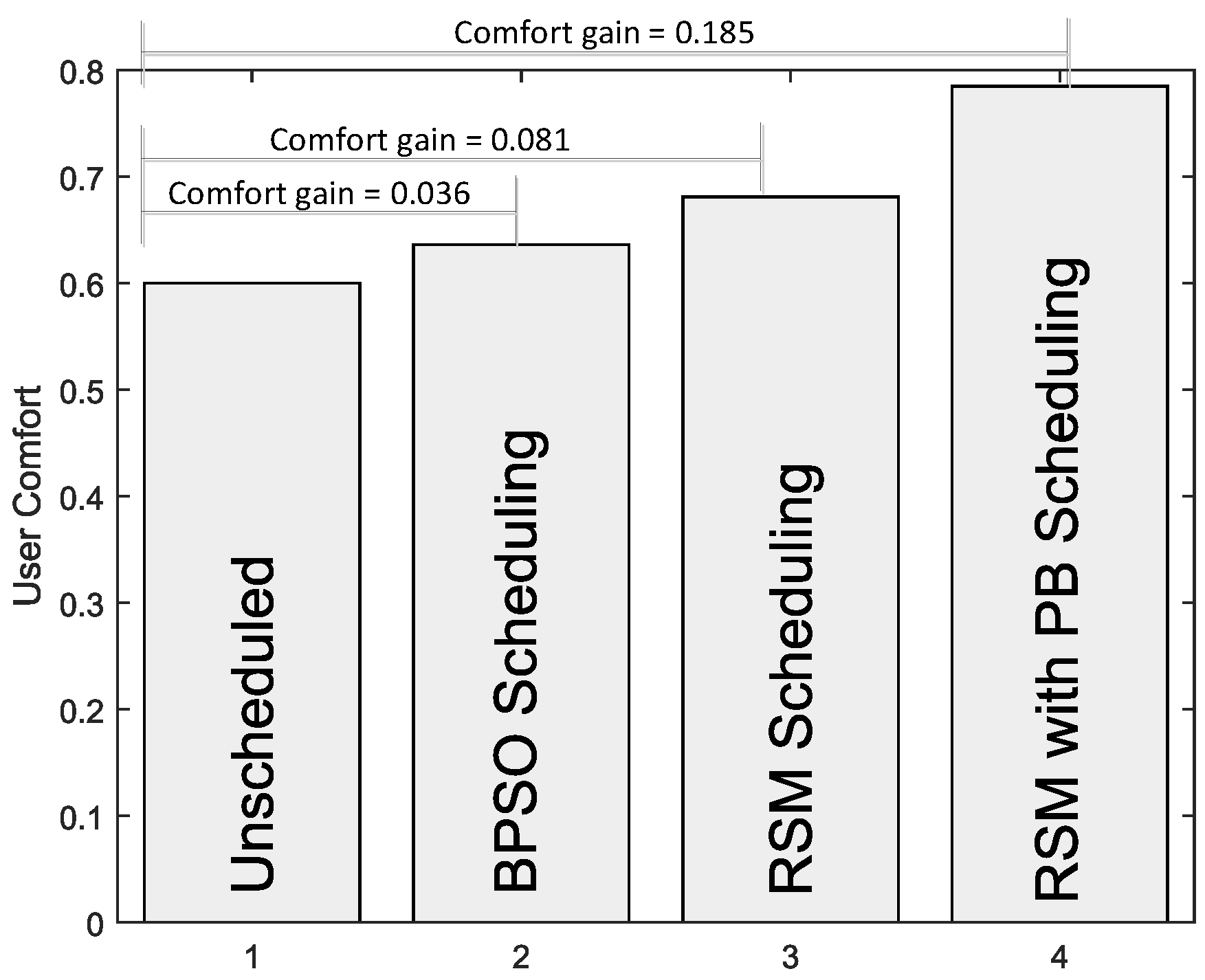
Scheduling home appliances in such a way that eliminates power demand peaks, intensifies UC and minimizes electricity bills having dynamic hourly electricity tariff is a basic problem. In literature, nature inspired heuristic algorithms are used widely to produce schedules that minimize electricity cost; however, achieving cost minimization by using such techniques often results in compromised appliance usage timings. This is because the scheduling horizon is vast and the algorithm has the liberty to schedule appliances within a 24 hour time span, raising user frustration. What if all RUs assemble their electric load on low price hours to save their electricity bills? The probability of increased demand with respect to supply will be higher, proceeding with higher probability of stifling the grid. Depicting UC, we define it as a state of equilibrium when the user has to pay lower electricity bills without effecting appliance utility or frustration level. Appliance utility refers to the use of electrical appliance within the desired range of time.
Therefore, the objective to achieve is to develop a balance between cost effectiveness and appliance utility up to user satisfaction level along with designing a dynamic power usage limiter that is also beneficial to electricity consumers and suppliers.
To achieve these goals, four major aspects are taken under deliberation; home occupancy, desired time of use of appliances, electricity price at time of use of appliance, and appliance utility with their specific constraints. Based on these parameters, we formulate RSM that classifies household electrical appliances and scheduling window, reducing electricity cost and elevating appliance utility. Scheduling window refers to the time span in which a set of appliances are meant to be scheduled. For each scheduling window, RSM uses BPSO keeping objective of cost minimization.
RSM is composed of algorithms regarding appliance functioning and operability that are utilized by a time modelling algorithm. Appliance classification is depleted by considering utility timings, nature of appliance and human presence. One long time slot (24 h) is divided into four logical sub-time slots that limit scheduling horizon. Each sub-time slot has six mini-time slots of one hour each. In limited scheduling horizon (sub-time slot), only one set of appliances is scheduled, raising appliance utility up to user satisfaction level (to ensure appliance utility part of UC).
For scheduling purposes, we apply BPSO keeping the objective function of minimizing cost for each sub-time slot contemplating electricity price, set of appliances to be scheduled and dynamic power threshold range deliberating PC during each respective sub-time slot. Although computational load increases, it also provides effective scheduling that takes care of user frustration as well as cost effectiveness. Our major contributions in formulating RSM are: (i) appliance classification and functioning algorithms with effective constraints, (ii) packet formats regarding all classes of appliances, (iii) dynamic power limiting threshold range with respect to electricity tariff, and (iv) optimizing scheduling horizon.
One cannot achieve an ideal condition in solving any complex problem. In our proposed scheme, we have to pay a price in terms of computational load. However, this cost is negligible considering the benefits that are achieved. Electricity consumers can have a dedicated processor for scheduling rather than relying on the processing power of a smart meter.
3. System Model: RSM
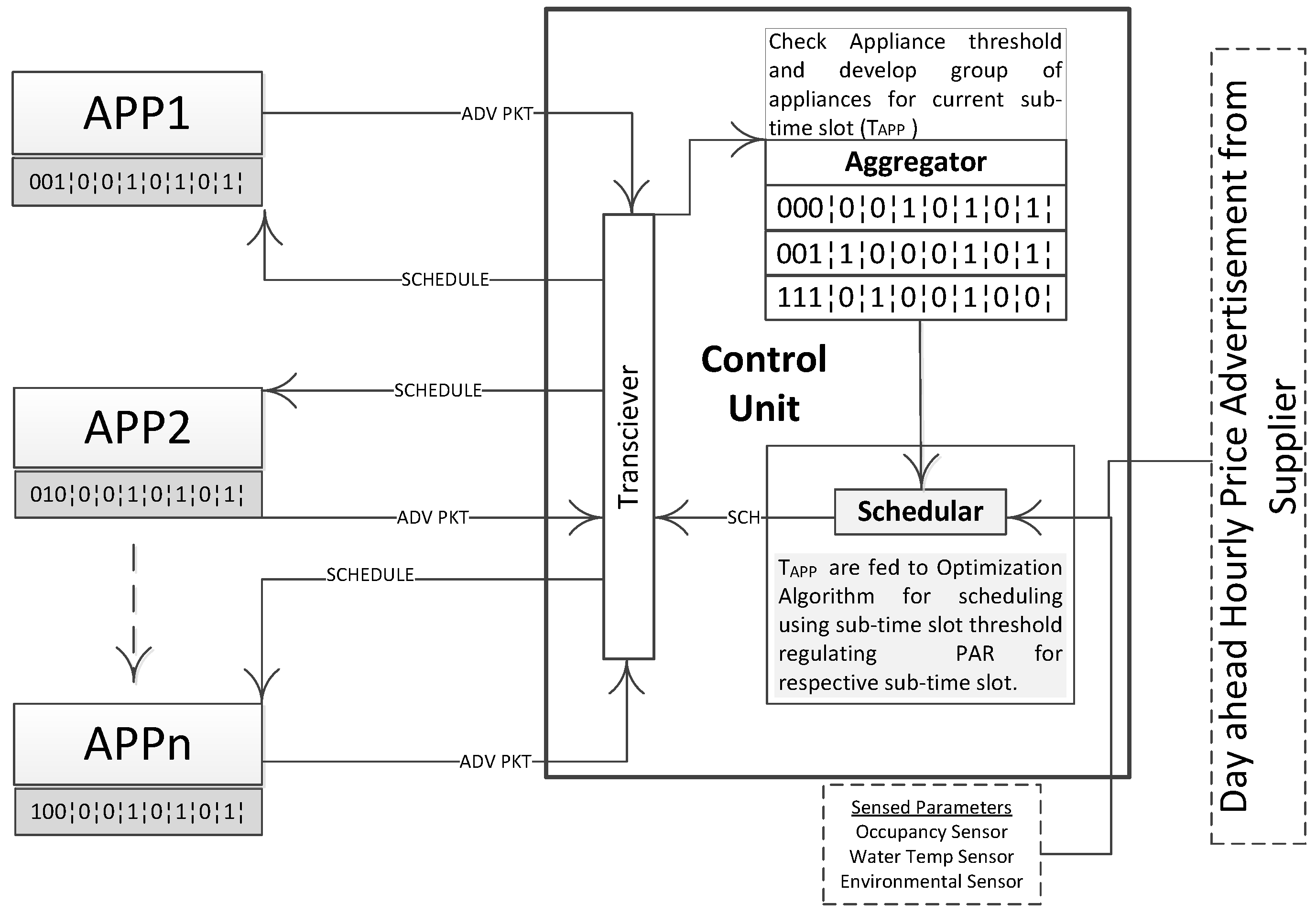
To develop an efficient HEMS, four entities,
i.e., the price at time, the TU, UA in RU and the nature of appliance are key players. A complete system model is defined as in
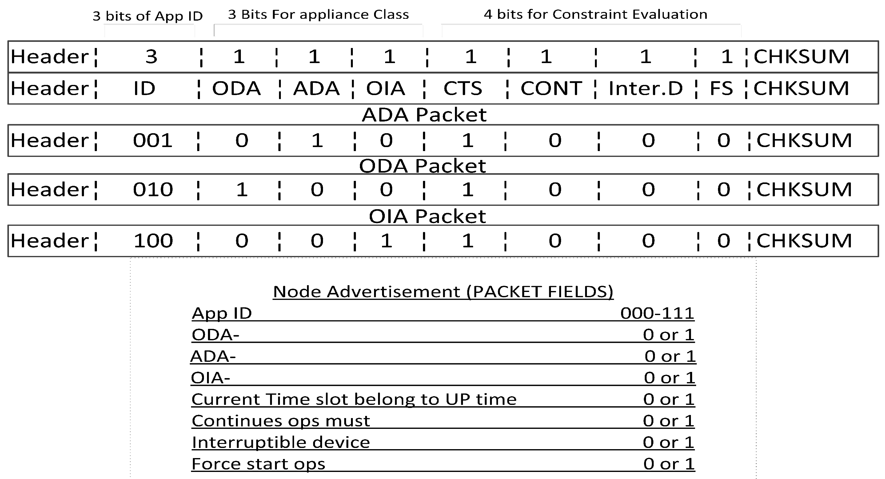
Figure 1 that takes care of said parameters. We consider a home having single occupancy with 10 smart appliances, that can be scheduled. We assume that every appliance is a smart appliance and has a built in sensor for different operations. Moreover, there is a network of sensors that sense different attributes regarding water tank for WP, water temperature for EWH, environmental temperature for HVAC and HO sensors. These sensors communicate their sensed value to control unit. Each appliance establishes its profile in form of a control/advertisement packet, that is transmitted to a scheduler. This advertisement packet has eight fields and is composed of 10 bits as shown in
Figure 1 and explicitly in
Figure 2.
The first field is of appliance
composed of three bits. In next three bits, it is determined that the appliance belongs to ADA, ODA or OIA class (explained in
SubSection 3.1). The fifth field informs us if the appliance is to be scheduled in this sub-time slot as per the user’s preferred time or not. The next field in the advertisement packet is responsible for determining whether the appliance needs a continuous operation without any deferment or not. The seventh field suggests that the device is interruptible or not, while last bit decides an opportunity of a force start regardless of time and final schedule made. The time frame, 24 hour time span, is divided into four equal sized sub-time slots, reducing scheduling window size.
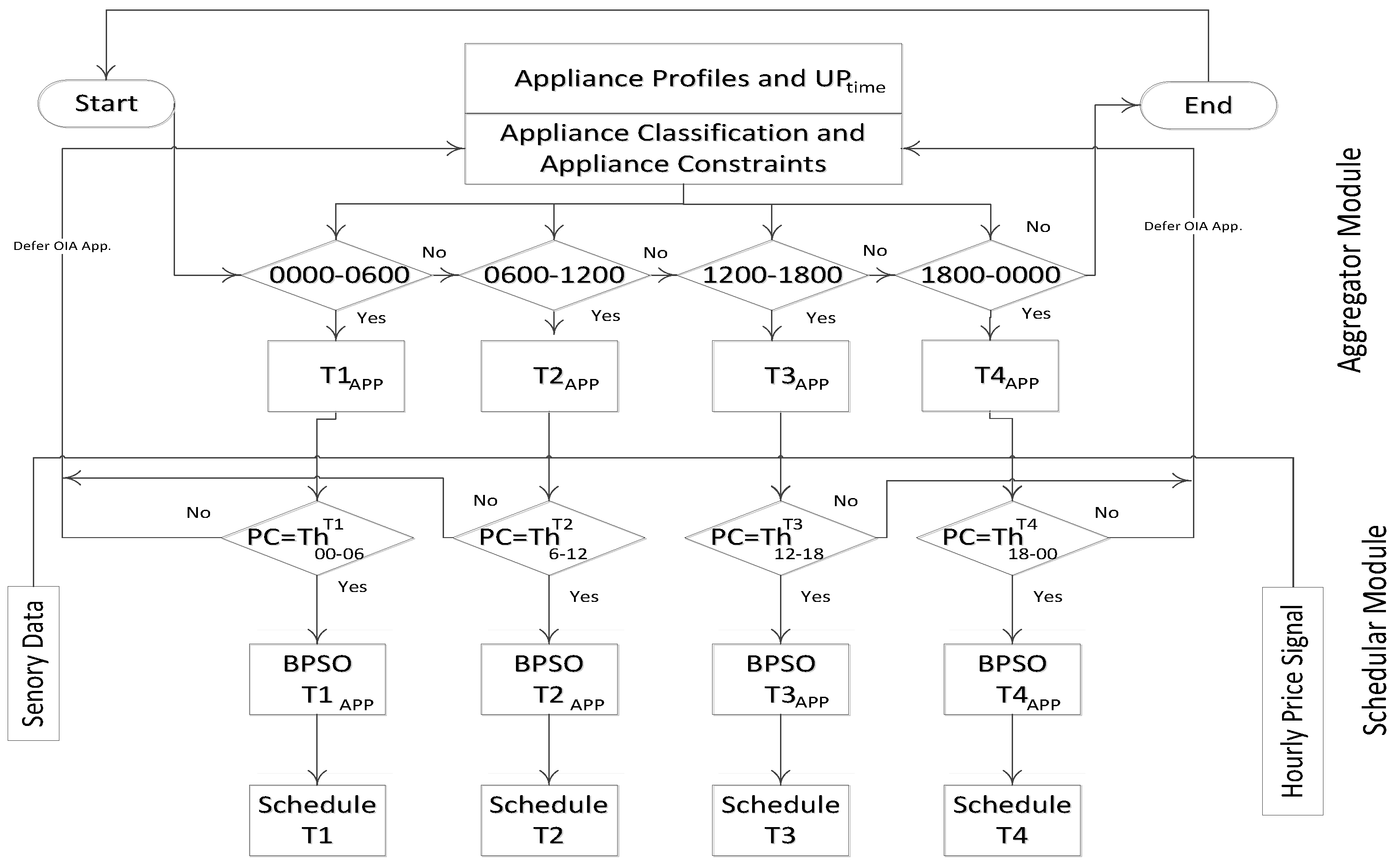
These profiles are gathered at aggregator modules of the control unit. An aggregator module collects these profiles, make sets of appliances regarding respective sub-time slots and verifies appliance threshold for the TU of appliance. These grouped profiles (for four different sub-time slots) are finally fed to the scheduler module of control unit. Prior to these profiles, the scheduler module has two more inputs, i.e., the day ahead price signal from electricity supplier and sensory data regarding environment (temperature outside and inside RU), water temperature in tank and HO. The schedular module also applies the sub-time slot threshold range to normalize the PC peaks.
Once appliance, time, threshold and PC modeling is done, we apply BPSO on each sub-time slot to get appliance schedule as
Figure 3 representing operability of RSM explains. Considering flow chart illustrated in
Figure 3, initially
and
is compared and a sub-time slot is found. Then a set of appliances for that sub-time slot is formulated by using appliance classification algorithms and profiles of each appliance. A power normalizing threshold for each appliance (using Equation (5)) plays an important role for selecting
along with
. Afterwards, PC limiter is applied using Equation (9) for the whole of the sub-time slot. This maintains the PC balance for both electricity user and provider. Finally, to achieve the objective of minimizing electricity bills, objective functions are fed to BPSO anticipating respective constraints to provide schedules that are user as well as supplier friendly. In this work we have not dealt with efficiency of communication protocol which is used between smart appliances and control unit. We assume that communication protocol works ideally.
3.1. Appliance Modelling
Classifying appliances, reflecting the said problem, is a complex task. Classification of appliances deals directly with appliance utility as well as cost effectiveness. Regarding appliance modeling, TU, PC and OA are focused parameters. Based on these parameters, RU’s electrical appliances are classified as
ADA: This class belongs to those appliances that not only require home presence but also need some activity performed on them. MO, IR, TV, etc., fall in this class.
ODA: These appliances are the ones that need human presence in RU to be operated. Such devices that are operable only if a home is occupied, fall in this class. For instance, what need is there for HVAC if home is vacant? It is also not necessary to switch on HVAC just on finding a low price hour without considering environmental temperature. Lights, EWH, etc., are the examples of this class.
OIA: The appliances that can be operable without home presence belong to this class. These appliances are delay tolerant and are meant to be scheduled at low price hours. WM, CD, PB, DW, WP, etc., are some examples of this class which are taken under consideration in this work.
With respect to described parameters and classification of electrical appliances, we can define each appliance separately. It is observed that, low PC appliances do not contribute significantly in high peaks of electricity demand. High PC devices play a vital role in generating peaks of electricity consumption. This is the reason that we take more high PC appliances as a prototype with respect to low PC devices.
Figure 4 depicts the algorithms that are designed for appliance workability raising appliance utility. Each appliance define its class in advertisement packet. The user also defines desired TU of that appliance. It is obvious that all appliances are not needed all together at the same instance. Moreover, an appliance may work multiple times in 24 h span as HVAC, MO and Ls,
etc. Algorithms for each class are explained in following subsections.
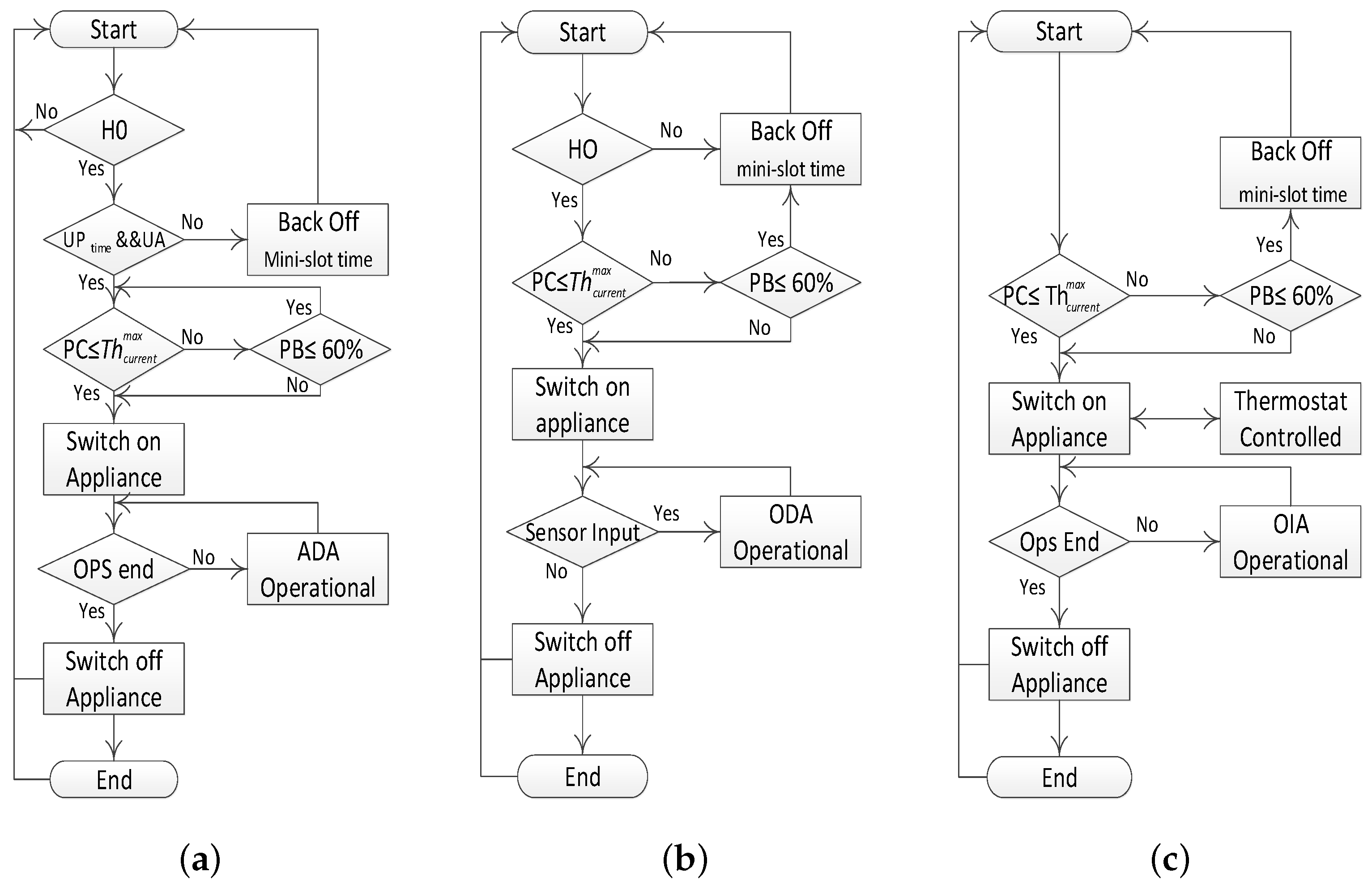
3.1.1. ADA Modelling
The most important class of appliances that plays vital role in user frustration or comfort is ADA. These appliances as the name indicates needs home presence as well as respective activity performed on that appliances.
Reflecting
Figure 4a there are four major thresholds,
i.e., HO, desired TU, UA and a PC limit (using Equation (5)). Analysing the algorithm for ADA class, it initializes and checks human presence if, occupancy sensor defines home presence, it will further proceed, otherwise, it will initialize again after a random back off time. If HO is verified, algorithm checks the desired TU and UA of this device. After passing these checks, an algorithm will check PC threshold, otherwise, an algorithm will be set to initialize again after a random back off period. Considering PC threshold check, it checks the overall PC at that specific instance. If it is below the predefined limit (
SubSection 3.3), then the appliance will be switched on. If PC, at that instance is higher than power usage limit, the appliance will switch on using PB considering charge on its batteries. These are the conditions which are common amongst the whole appliance range of ADA class. However, each device may have some of its own constraints which are elaborated in a periodic control packet. These limitations tend to raise UC and efficiency in terms of electricity usage.
Normally, a home is occupied for the evening, night and morning time. Electricity appliances of this class are needed mostly in the morning when the user has to prepare for the office and evening when the user comes back from the office. Focusing MO as a vital appliance of ADA, it can remain in ONS, OFS and WS while, state 00 refers to OFS, 10 is WS and 11 defines ONS.
At a given instance of time, MO can be in any of above mentioned state. To register in WS or ONS (Equation (1)), the following constraints must be analyzed.
| Conditions : |
| 1: |
| 2: if && && ϵ then |
| 3: |
| 4: if then |
| 5: |
| 6: end if |
| 7: if && then |
| 8: |
| 9: |
| 10: end if |
| 11: if then |
| 12: |
| 13: else |
| 14: if && then |
| 15: |
| 16: end if |
| 17: end if |
| 18: if then |
| 19: |
| 20: MO==10 |
| 21: end if |
| 22: |
| 23: end if |
Line 1 expresses the 00 state of microwave oven and it will shift to 11 state if the home occupancy sensor senses presence in the home, and current time slot is the desired time slot. Moreover, some user activity is planned in this time slot as depicted in line 2. In this document, 1stands for yes or on, while 0 represents no or off. State 11 shifts to state 10 if, power consumption is lower than the threshold of that particular mini-time slot. Considering line 8, if power consumption of the mini-time slot is exceeding the threshold limit, then PB will be consulted. If charge in PB is greater than MO will set in state 10 while PB is shifted to state 10. There is another check, regarding switching to 10 state, i.e., if in advertisement packet or if the option of force start is on, the appliance will be set to 10 state at the prescribed time regardless of PC (line 12). However, if force start option is not set on, and PB charge is less than , MO will remain in 11 state until PC threshold is satisfied (line 15). Mostly, food is cooked by giving proper attention. The higher the temperature setting of MO is, the higher will be the power consumption resulting in higher power demand. Line 20 limits the temperature range into an upper and lower bound of temperatures, where x and y are the desired limits of MO set by the user. The delay for this appliance is set as 120 min.
3.1.2. ODA Modeling
These are the devices which are needed only when a home is occupied, as the name indicates. Many appliances may fall in this class like HVAC, EWH, Ls,
etc. Figure 4b narrates ODA class of appliances, it deals with only three thresholds,
i.e., checks the HO,
and PC at that instance. This algorithm follows the same procedure as that of ADA class, the only difference is, that it does not precisely follow the user preferred time during respective sub-time slot. It checks different parameters depicted by environmental and temperature sensors. As discussed earlier, these are general conditions that are valid on every ODA. There can be some other constraints on a device level to further optimize the solution.
Let us anticipate that EWH belongs to ODA class, i.e., . Performance of EWH depends on hot water storage tank. We assume that tank can contain x litres of water and can keep water warm for T minutes. Moreover, EWH warms x litres of water in time, consuming power. EWH can be in OFS, ONS or WS where 00 represents OFS, 10 shows WS of appliance and 11 stands for ONS of Appliance.
Framework of EWH is presented in Equation (2):
| Conditions : |
| 1: |
| 2: if && ϵ then |
| 3: |
| 4: if then |
| 5: |
| 6: end if |
| 7: if && then |
| 8: |
| 9: end if |
| 10: if && then |
| 11: |
| 12: |
| 13: end if |
| 14: if then |
| 15: |
| 16: else |
| 17: if && then |
| 18: |
| 19: end if |
| 20: end if |
| 21: if then |
| 22: |
| 23: |
| 24: end if |
| 25: |
| 26: end if |
Anticipating EWH that belongs to ODA, the initial state is 00 will shift to 11 state if the HO sensor is positive and current sub-time slot is the desired time slot. To shift to state 10, water temperature range is verified as in line 4. If current water temperature rests within the range, state 11 will continue otherwise, as depicted in line 8 to 16, PC threshold is checked, PB state of charge is verified and force start option is checked as being to set to state 10. If force start option is not set on while charge on PB is less then
, EWH will remain in WS until above mentioned constraints are fulfilled. Delay is set to 180 min for this appliance (within 6 h of sub-time slot) as ODA class does not require urgent attention and can be utilized to minimize electricity bills without effecting appliance utility. It is assumed that water tank has the ability to keep water warm for 5 h and comfortably usable for 3 h. Hence, it can be switched on 180 min prior to usage time. This is the time limit where water remains usable without any discomfort. Focusing EWH, it is required only in morning time, hence, it can be scheduled at times such that line 27 is satisfied. In the same way, appliances that lie in ODA class will have almost the same constraints, given that they may have different tolerance levels and comfort zones,
i.e., for HVAC, there will some different range of temperature to be set and have to analyse outside along with inside temperature of RU.
Figure 2 illustrates advertisement packet format representing ODA class as well.
3.1.3. OIA Modelling
OIA class of appliances are independent of human presence. All they require are certain control signals to become operational without any human interference. OIA class as illustrated in
Figure 4c checks only power threshold value. If there is a room for said device to switch on, the algorithm turns that appliance on. This class of appliances mainly shaves electricity demand peaks and resolve different conflicts of TUs regarding other two classes.
We take PB as prototype for this class of appliances. This device can be in three states, i.e., 00 states its OFS, 01 represents CS while 10 refers to its DS.
If PB is in 00 state, it means that normal operation is ongoing. Electricity from supplier is utilized and PB is in OFS. 01 state informs CS of PB. It reflects the time, when batteries are charging
i.e., that must be a low pricing hour. Moreover, this is an OIA, hence it can be operational at any instance, once given constraints are fulfilled. 10 state represents DS. Discharging of batteries happen only when it is necessary to use electricity while the electricity price offered from the supplier is high, or needed electric load is exceeding PC limit. During peak pricing hours or peak demand hours, the probability of DS considering PB is maximal than CS. PB framework is presented in Equation (3):
| Conditions : |
| 1: |
| 2: if && then |
| 3: |
| 4: end if |
| 5: if && then |
| 6: |
| 7: end if |
| 8: if && && then |
| 9: |
| 10: end if |
The initial state of PB is 00 which will remain if the PC of the mini-time slot is less than the PC threshold and charge on PB is greater than or equal to as in line 2. Line 5 expresses that if PC exceeds the threshold and is greater than or equal to , PB state is set to 10 i.e., discharging state. This means, to remain under threshold level, some of the appliances will start consuming power from PB to minimize grid billing at high load hour. PB is a dual natured appliance, it serves as a mini MG while in 10 state and acts as an ordinary appliance during 01 state. The user defines its operational time (01 state) for charging. If the charge on PB is less than along with PC is under threshold, the state of PB will shift to 01. This OIA needs high electric power to operate; however, it also gives relief to the user in high price and load hours. HEMS may shift some of the load on batteries to ensure appliance utility, PC peaks reduction and lower bills. We assume that RU is equipped with an RE source. This RE scourge charges PB along with two hours of further charging by using electricity provided by the supplier. In this way it is capable of storing of the consumed power and helps in lowering electricity consumption/ billing at high pricing hours. Modelling RE expenditures (Power storage system, installation cost of RE source/s and maintenance around its life cycle) will be dealt with in future works.
3.2. Time Modelling
Scheduling horizon plays an important role in appliance utility and cost minimization. It has a direct influence: as the scheduling horizon is widened, cost will decrease proportionally. However, appliance utility is compromised likewise. Limiting scheduling horizon may lead to less cost effectiveness but it will raise the appliance utility. To include cost effectiveness in limited scheduling horizon, effective appliance grouping representing each logical sub-time slot, will lead to minimized electricity bills.
We, in this work, divide 24 hour time into four prominent sub-time slots i.e., from 00:00 to 06:00 as , from 06:00 to 12:00 as , 12:00 to 18:00 as and 18:00 to 00:00 as . We categorize these sub-time slots in accordance with daily routine pattern commonly observed at a normal RU. Each sub-time slot is further decomposed into six equal sized mini-time slots of one hour each. Scheduling window is minimized to a sub-time slot. Hence, there are four scheduling windows within time frame of 24 h.
During any specific interval of time, all the n appliances are not needed. There may be a group of appliances that is operational. Moreover, limiting scheduling window along with precisely developed set of appliances to be used in this sub-time slot, results in more effective scheduling. It is not necessary that an appliance that ∈ n works only in one sub-time slot. It may be utilized time and again, such as MO or HVAC. For the said reason, we state that, there are “n” appliances in an RU. During , a set of appliances are to be scheduled. While in , are in use, similarly and are operational in and sub-time slots respectively. Where , , and . Subset a is set of those appliances, that are elected to be in OFS for sub-time slot . Likewise, sets (b), (c), (d) are sub sets of appliances that belongs to super set n of all electrical smart devices but not lie in , and respectively. These subsets are formed by appliance profiles and . Sets of appliances for sub-time slots are made focusing , appliance profiles and appliance threshold, without considering classification of appliances.
Resident of the home inputs his
and duration of use reflecting any specific appliance. A set of appliances that is to be used in certain sub-time slot (
i.e.,
) is based upon the appliance classification mechanism as discussed in
Section 3. Mathematically we can state as in Equation (4):
such that
where
.
defines the sub-time slot of appliances within 24 h time frame.
is time of use of appliances that exists in set(a). These sets are formed on checking TU with respect to the next sub-time slot and are variable so that any appliance can work in more then one sub-time slots as per user requirement. Considering any set of appliances,
i.e.,
, appliances can deviate within respective mini-slot times of one sub-time slot; however, they are not supposed to shift their sub-tim slot, to avoid user discomfort.
3.3. Power Threshold Framework
Limiting power usage and creating a threshold is one of the most critical parts of an effective HEMS. Threshold if modeled carefully, plays an important role in maintaining an equilibrium that not only is beneficial to electricity consumer, but also for power suppliers by stabilizing the smart grid. The grid is vulnerable on high price hours as well as low price hours. It is obvious that at high price or load hours, the grid may choke. While, if consumers shift their electric loads collectively on low pricing hours, this again will result in choking of electricity supplying company. To tackle these two extremes, an efficient power threshold mechanism is needed that regulates electricity usage.
To accomplish this, we devise two types of thresholds,
i.e., appliance threshold and sub-time slot threshold range. For appliance threshold, that is required while switching on any electrical device, we calculate it on the basis of unit price of electricity at that certain hour. This threshold changes as the price of hour changes. Hence, it regulates high demand curves at low or high price hours dynamically, as shown in Equation (5):
stands for the threshold calculated for the current hour.
is consumption of electricity (in
) by all electricity appliances that are to be scheduled in that sub-time slot. Whereas
depicts the electricity cost of respective hour issued by electricity supplier.
x is a variable that can be changed according to needs of electricity consumer. This increases the threshold value of power consumption per hour as per need. We define
x as 1.5 in this work.
is utilized in algorithms that define functionality and operability of electrical appliances (
SubSection 3.1).
To calculate maximum electricity consumption, we use Equation (6):
Equation (6) gives the sum of PC by all active appliances in specific mini-time slot. Where stands for the kilowatt per hour PC by an appliance and is number of appliances that are determined for that specific mini-time slot.
The lower boundary of threshold is represented as
and can be calculated as in Equation (7):
where:
PC range for an hour can be calculated as the difference between
and
. Mathematically it can be represented as in Equation (9):
Equation (9) gives PC range of specific hour that deviates between
and
. Per hour maximum and minimum thresholds are defined in Equation (5) and Equation (7) respectively. We use Equation (5) in appliance modelling (
Section 3 for switching on an appliance). However, during a sub-time slot, it is not necessary that every hour of the sub-time slot must be occupied even if there is no need to utilize any appliance. For that we need a maximum and minimum threshold value for whole sub-time slot,
i.e., six mini-time slots. During these 6 h (mini-time slots), there may be hours where the state of “
no electricity consumption” can be achieved without generating PC peaks in other mini-slot times of respective sub-time slot.
Hence for sub-time slot threshold, we calculate minimum and maximum electricity to be utilized in whole sub-time slot (Equation (11) and Equation (12) respectively). That defines the threshold range for specific sub-time slot as in Equation (10):
where,
and
represents the avarage price during sub-time slot. To calculate maximum and minimum range of PC during a sub-time slot, we use Equation (13) and Equation (14) respectively.
3.4. Power Utilization Framework
The day ahead RTP model is utilized that is published online day ahead. As said earlier, there are many devices that may switched off or are not in use with respect to that sub-time slot. Also, an appliance may be needed at multiple times during a day and occupancy of RU impacts directly on scheduling electrical devices. On the basis of presented modeling of electrical appliances, sub-time slots and power threshold range, we devise PC cost profiles for each sub-time slot in following subsections.
PC Cost During the Allocated Sub Time Slots
sub time slot refers to fist 6 h of the day where
= 00:00 and
= 06:00 having six mini-time slots of 1 hour each. During this sub-time slot, appliances under attention belongs to
. Scheduling time for
can be stated as in Equation (15):
The amount of power that is consumed during
by
set of appliances is represented in a vector form as:
where,
is the range of appliances that can be switched on during
hour of
. While,
to
refers to six mini-time slots of
. Sum of all the fields of vector (Equation (16)) yields PC of all appliances during
.
Equation (17) ensures that a certain range of power is permissible to be used. It gives maximum and minimum PC limit of
appliances during
time span.
As prices can vary every hour and are known to scheduler in advance, total PC cost during
is stated as:
We follow the same model as presented for in rest of the sub time slots; , , and .
3.5. Problem Formulation
Accumulative objective function for 24 hour time span “
T” is expressed in Equation (20):
Such that;
Constraint ’a’ represents the user preferred time for whole day logically dividing 24 hour into 4 equal sized time slots to enhance appliance utility (). The set of appliances formed for each sub-time slot is bound to be operational within respective sub-time slot as depicted in constraint ’b’, where, if , if , if , and if . A dynamic power limiting range is designed which is based upon HO, UA and price at time of use, enforces certain amount of PC during respective sub-time slot in constraint ’c’. In constraint c, and if , and if , and if , and and if . Whereas, constraint ’d’ tackles the probability of force start option of any appliance.
4. PSO
The PSO algorithm is dependent upon two major functions,
i.e., velocity update function and position update function [
28]. On every iteration, each particle is subject to move towards a previous best position or global best position. Hence, every new iteration brings new velocity of each particle along with distance of the global best position. This new velocity value is calculated to find next position in
n dimensional search space
s. Iterations keep repeating until the required solution is achieved. The velocity of a particle is obtained by using the Equation (21):
where
And for position update function, we use the Equation (23):
BPSO for RSM
BPSO is a variant of PSO, with the only difference that, decision variables are binary, i.e., zero and one. The objective function is fed to BPSO that develops schedule for respective sub-time slot considering UC focusing appliances usability and cost of electricity at time of use.
In BPSO, particles are initialized for binary positions randomly.
Position of each particle is defined by:
Table 4 represents the simulation control parameters of BPSO for scheduling home appliances.
Scheduling smart home’s electrical appliances by applying nature inspired heuristic algorithms is emerging topic amongst researchers and engineering industries. Vast literature exists that presents recent trends of using and modifying PSO, GA and ANN techniques for the said purpose, i.e., scheduling home appliances for cheaper electricity bills.
5. Simulated Results and Discussions
We consider an RU of a residential building, however, our proposed scheme can be implemented on any home or residential apartment. This RU has single occupancy, one bedroom, one living room, a kitchen and a washroom. For validation of our proposed system, we take assumption of an RU having 10 smart appliances. These appliances are connected to HEMS, while we have knowledge of hourly electricity tariff a day ahead.
Table 5 shows the appliances that belong to a specified class (user defined), duration of operation in 24 h time (user defined), duration of operation in specific sub-time slot (user defined based upon
) and their power rating as watt per hour (manufacturer rating). We take these listed appliances for scheduling, aiming to reduce user frustration and maximize appliance utility cost effectively, as discussed in above sections. In all of the mentioned appliances, role of PB is vital. We, in these experiments, include it as another device when it is required to be charged. For DS we calculate its impact which is vital. However, we do not include its technical specifications and assume that, if fully charged with the support of PV system, it can provide
of the load. Considering DR program type, we use day ahead dynamic hourly pricing scheme which is published by electricity company day ahead. In this section, 0 stands for the OFS of appliance while 1 respond to ONS of appliances due to the binary nature of applied optimization technique.
5.1. Scheduling Sub-time Slots
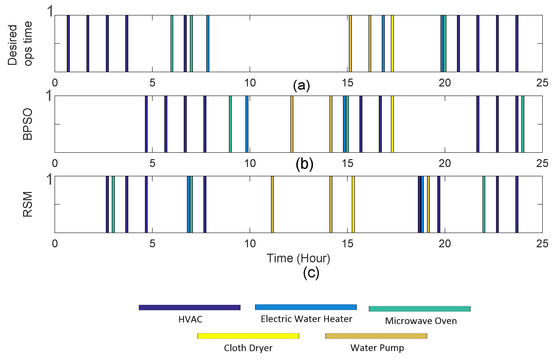
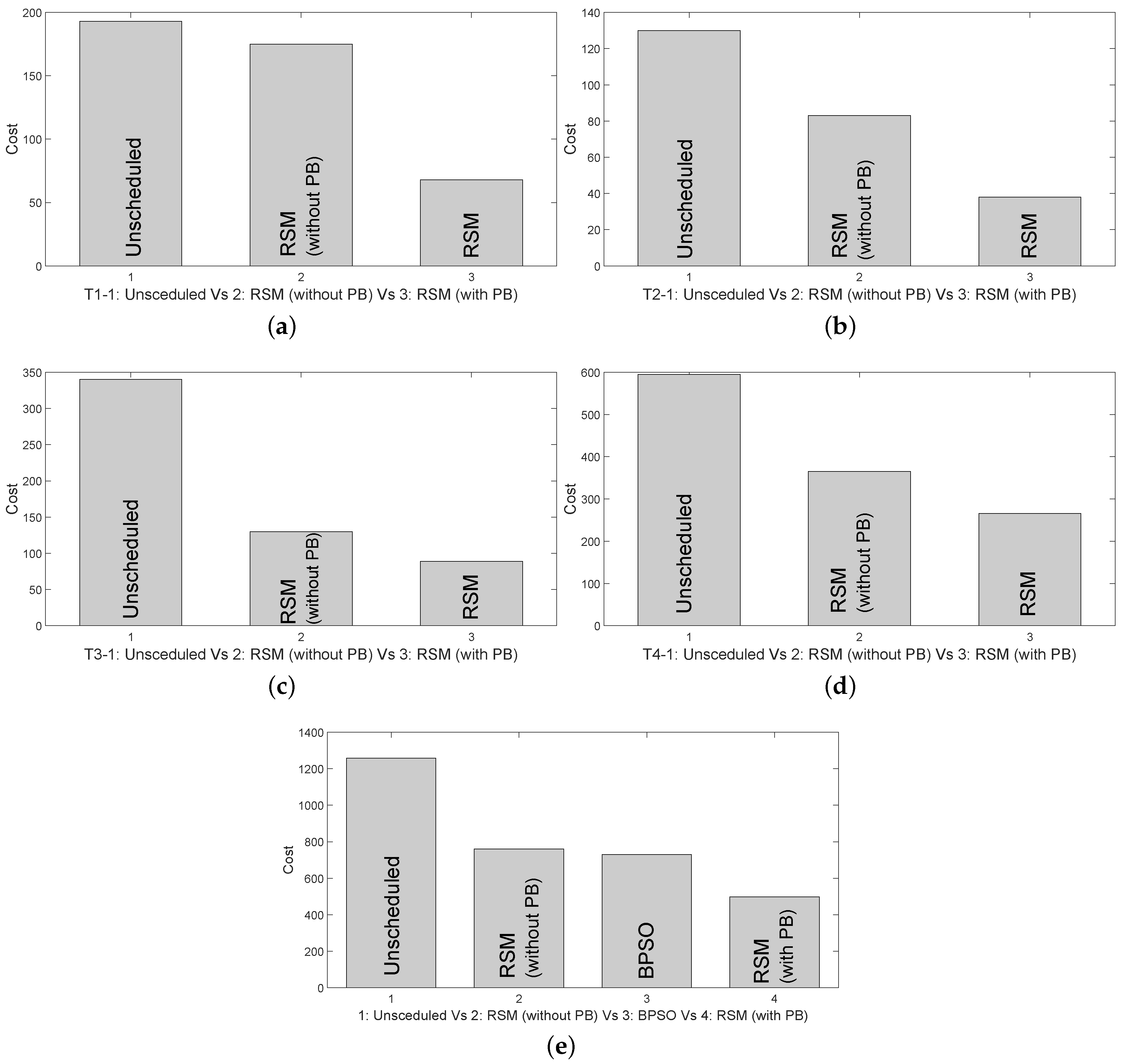
In the following subsections, results reflecting each sub-time slot are presented to analyze impact of RSM with respect to unscheduled. In the experiments, we also analyzed the role of PB in RSM which gives near to optimum results. In the following Subsections, we compared unscheduled, RSM without PB and RSM with PB for each sub-time slot.
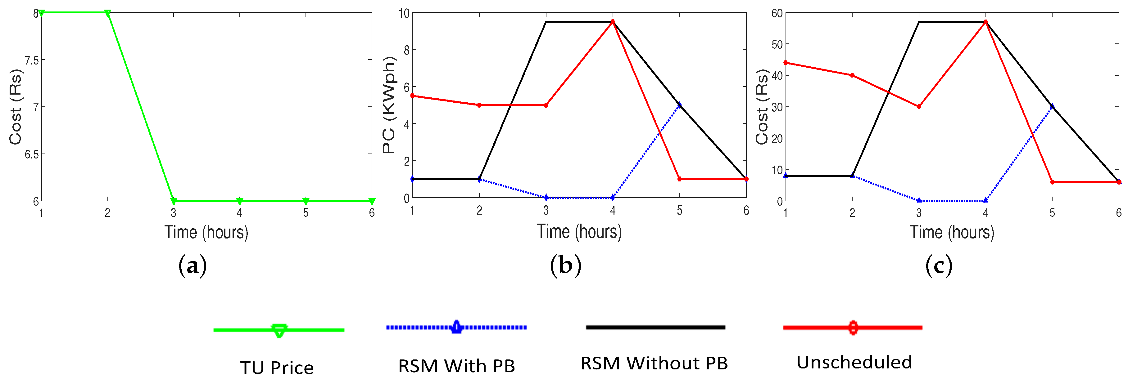
5.1.1. Scheduling
represents the time between 24:00 to 06:00. This is the time when home is occupied and occupants are normally taking their sleep. Hence, ODA class of appliances is dominant in
in accordance with
and electricity cost per respective hour. EWH, REF and HVAC,
etc. do not require special attention, but require HO. For EWH, user require 2 h of operation: one near midnight before going to bed and one right before getting out of bed. REF needs to be run continuously, however, it can be deferred for a maximum of one hour, if load is crossing the threshold. Hence, during this time span, Equation (25) expresses
set of appliances.
Figure 5a depicts the hourly price advertised for
.
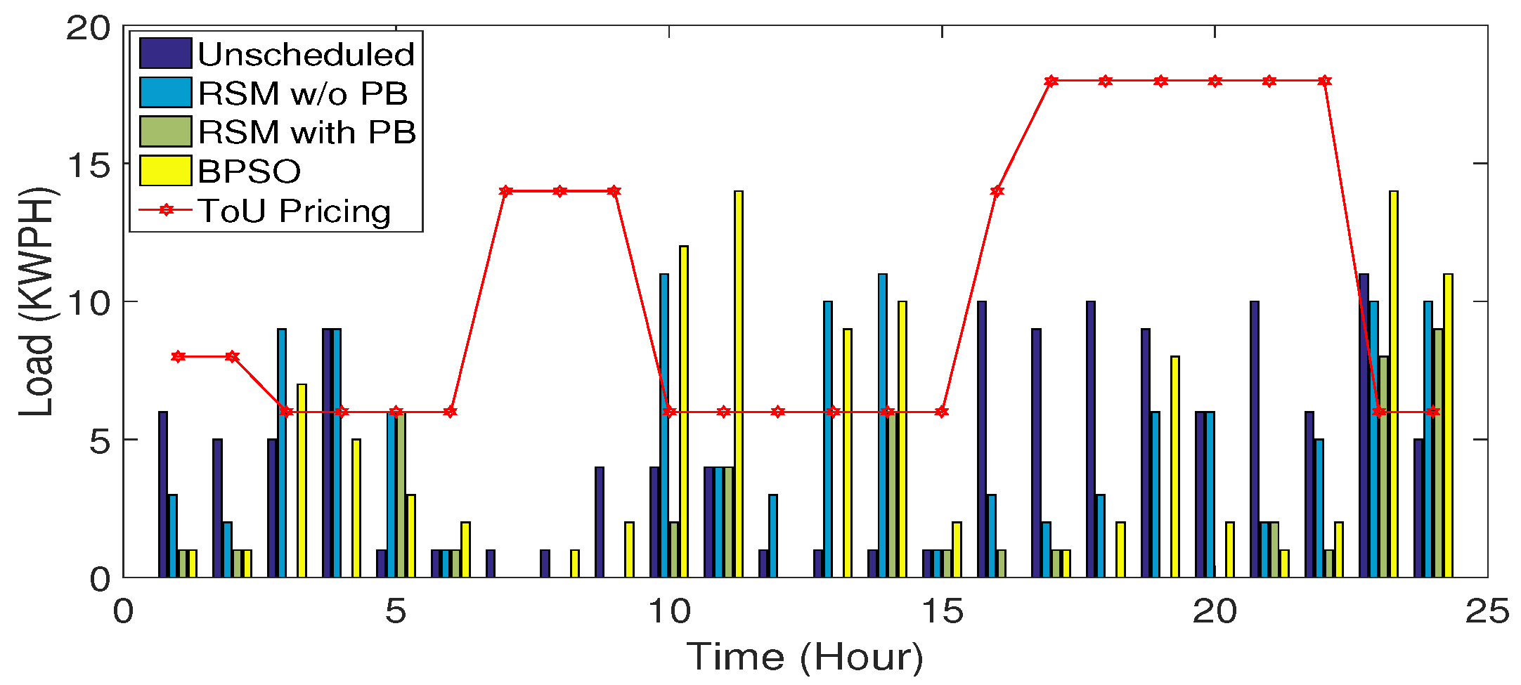
Figure 5b represents the PC pattern considering three approaches,
i.e., scheduling with the help of proposed mechanism (with and without PB) and unscheduled. We induced the impact of PB on electricity cost savings. As we can see in
Figure 5b,c, during the high price timings, electricity consumption was lower and during low pricing hours, electricity consumption was higher with respect to proposed scheme. However, using PB as a helping source of power at high cost timings, billing is minimum.
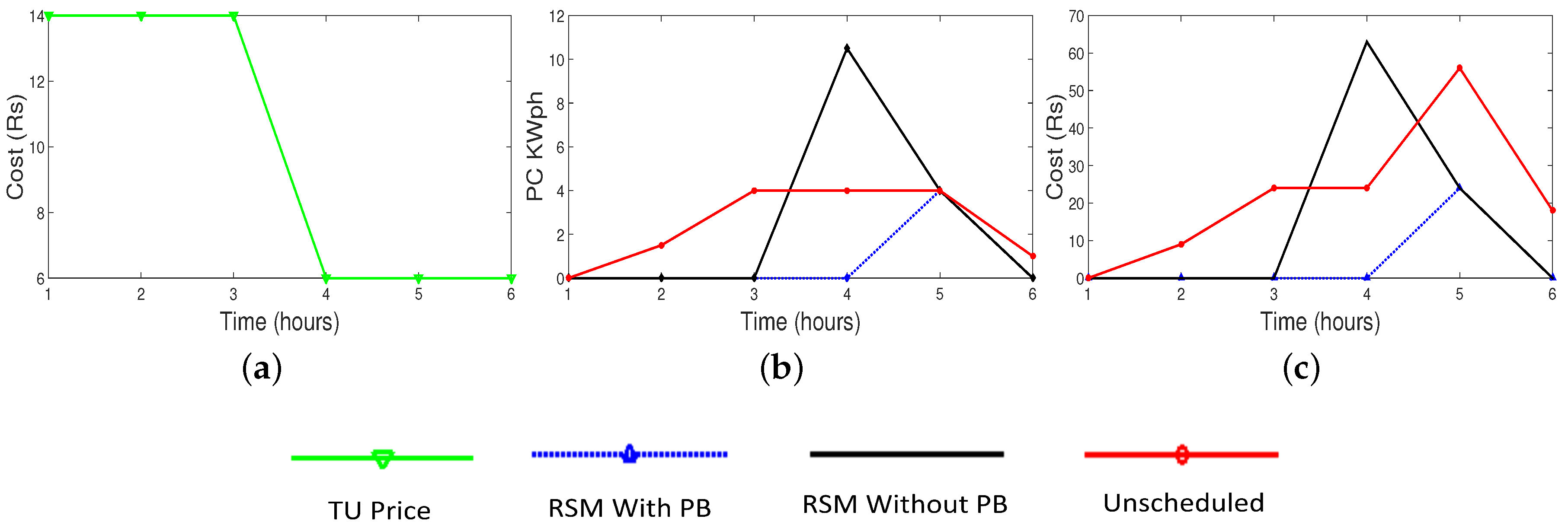
5.1.2. Scheduling
represents the time between 06:00 to 12:00. During the first half of the time, the home is occupied as the user gets up, and prepares to reach his work space. After 09:00 the home remains vacant. During the latter half, OIA is major class representing to ensure UC.
The price per hour of this sub-time slot can be seen in
Figure 6a. For the initial three hours,
i.e., from 06:00 to 09:00 the price is higher and afterwards, it is
per kilowatt for the rest of this sub-time slot. PC and cost comparison between scheduled load by RSM without PB, unscheduled load and scheduled by RSM with the support of PB is shown in
Figure 6b,c respectively. Without RSM, electricity consumption is higher at high price timings which is lower in scheduled load. At the time when prices are low, scheduled load is higher.
Equation (26) represents appliances in set.
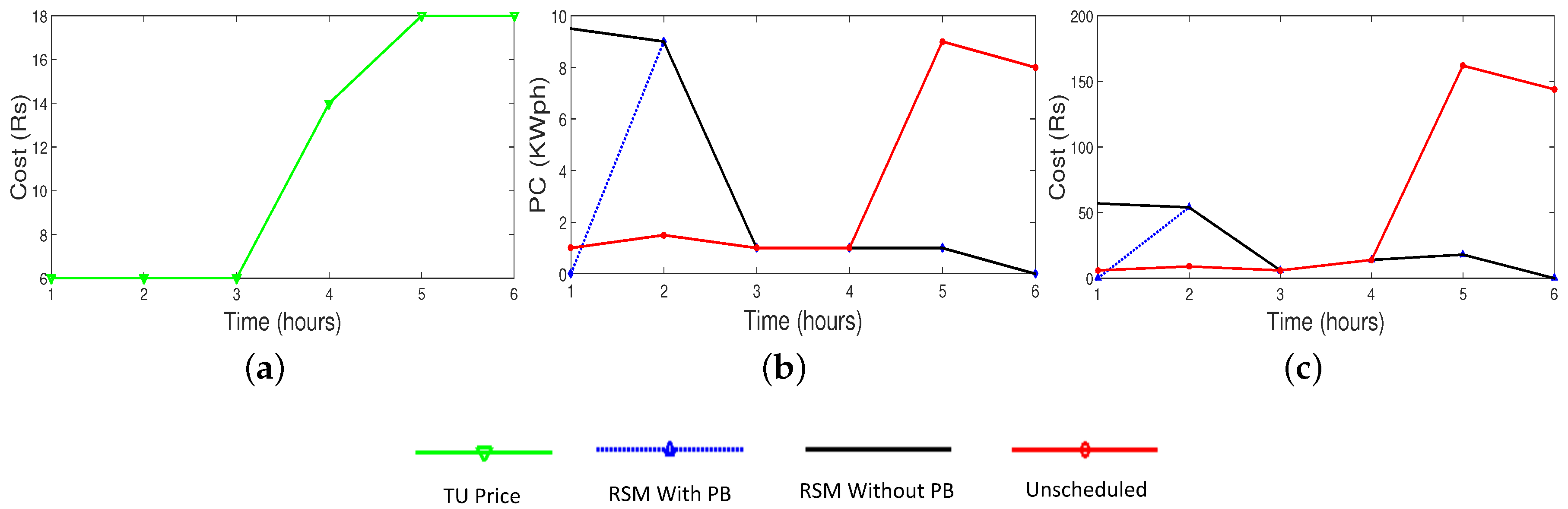
5.1.3. Scheduling
sub-time slot represents the time between 12:00 to 18:00. At this sub-time slot, OIA class of appliances is meant to be scheduled. Normally, office timings are 09:00 to 17:00 and so, the user may reach home after 17:00
h. During this time slot,
set based upon appliance profiles and
is given in Equation (27):
Figure 7a anticipates the tariff of this sub-time slot. From 12:00 to 15:00 tariff is
while from 15:00 to 18:00 the price is
and then
per kilowatt for last two hours. During high peak hours, minimum load is scheduled by RSM keeping in view that the home is vacant and maximum load is shifted to low price hours to preserve electricity.
set is formulated considering appliance classification and
maximizing appliance utility as well as cost savings. On the other side, unscheduled load consume electric power regardless of electricity pricing as shown in
Figure 7b.
Figure 7c presents the price comparisons between scheduled with RSM, Scheduled RSM with PB and unscheduled load. During high price hours, price is minimal with respect to unscheduled load.
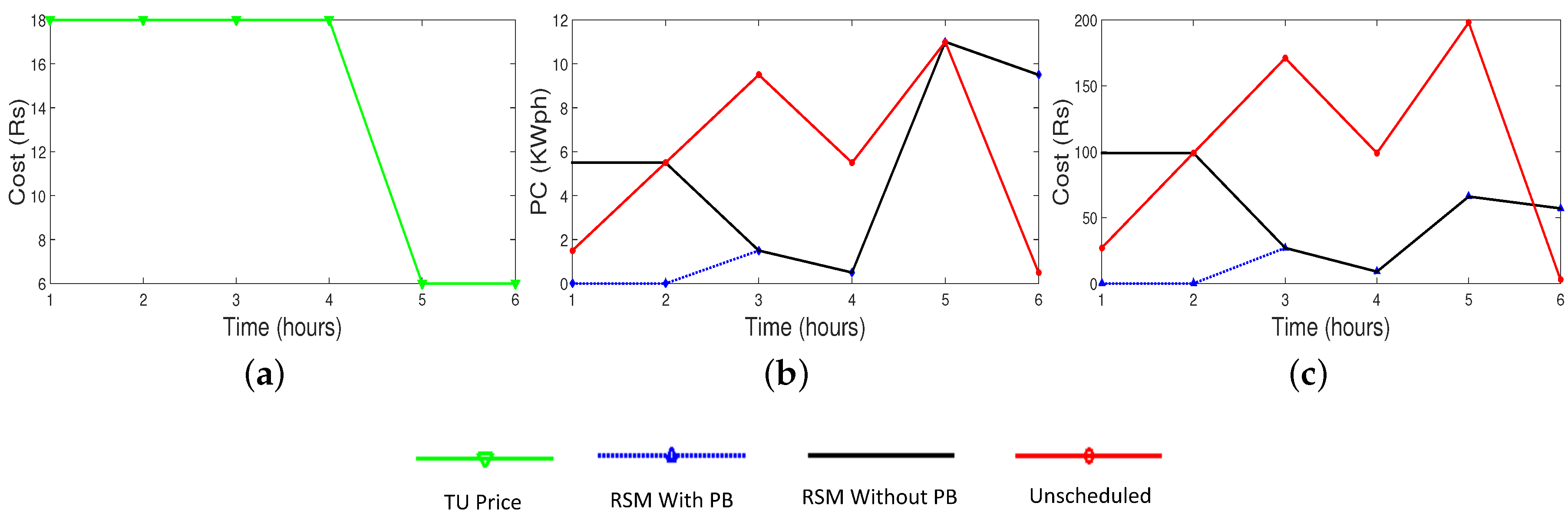
5.1.4. Scheduling
represents 18:00 to 24:00. This sub-time slot can be termed as most active sub-time slot of all, as user is available and can turn on any appliance according to his need. Hence appliances from all classes,
i.e., OIA, ODA and ADA classes are prominent members of set
as Equation (28) shows:
Figure 8a depicts the price hours of this sub-time slot. Initial hours are the peak pricing hours whereas price is lower after 22:00. If we analyse PC in this sub-time slot,
Figure 8b states that during high pricing hours scheduled load tends to decline however at cheap hours, the load is maximum. Observing unscheduled load, it raises to almost
during high price hours as can be seen in
Figure 8c. Likewise if we compare pricing of these two approaches,
Figure 8c clearly states that scheduled cost is much lower than unscheduled cost.


 ,
, 


