Cost Engineering Techniques and Their Applicability for Cost Estimation of Organic Rankine Cycle Systems

Abstract

The potential of organic Rankine cycle (ORC) systems is acknowledged by both considerable research and development efforts and an increasing number of applications. Most research aims at improving ORC systems through technical performance optimization of various cycle architectures and working fluids. The assessment and optimization of technical feasibility is at the core of ORC development. Nonetheless, economic feasibility is often decisive when it comes down to considering practical instalments, and therefore an increasing number of publications include an estimate of the costs of the designed ORC system. Various methods are used to estimate ORC costs but the resulting values are rarely discussed with respect to accuracy and validity. The aim of this paper is to provide insight into the methods used to estimate these costs and open the discussion about the interpretation of these results. A review of cost engineering practices shows there has been a long tradition of industrial cost estimation. Several techniques have been developed, but the expected accuracy range of the best techniques used in research varies between 10% and 30%. The quality of the estimates could be improved by establishing up-to-date correlations for the ORC industry in particular. Secondly, the rapidly growing ORC cost literature is briefly reviewed. A graph summarizing the estimated ORC investment costs displays a pattern of decreasing costs for increasing power output. Knowledge on the actual costs of real ORC modules and projects remains scarce. Finally, the investment costs of a known heat recovery ORC system are discussed and the methodologies and accuracies of several approaches are demonstrated using this case as benchmark. The best results are obtained with factorial estimation techniques such as the module costing technique, but the accuracies may diverge by up to +30%. Development of correlations and multiplication factors for ORC technology in particular is likely to improve the quality of the estimates.

1. Introduction

Organic Rankine cycle (ORC) technology increasingly draws the attention of researchers and practitioners. The concept of using an organic fluid instead of water dates back to just after the invention of the conventional Rankine cycle in 1859, yet it was not until the 1960s and 1970s that ORC technology was investigated more prominently. Today, the ORC constitutes a flourishing research field and its practical potential has been proven. The advantages of ORC systems are manifold. Operating with organic fluids allows conversion of energy sources in much lower temperature ranges than feasible with conventional steam cycles. ORC systems can thus generate electricity from excess heat, enhancing energy efficiency, and from geothermal wells, biomass, solar and oceanic sources. Both enhanced efficiency of energy use and renewable electricity generation are essential in the transition of energy sectors to more streamlined, efficient, secure and climate-friendly systems.

Research conducted on ORC technology and applications is very technical in nature. The majority of the literature is devoted to i.a. architecture design and optimization (e.g., Chen et al. [1], Lecompte et al. [2]), the quest for suitable working fluids (e.g., Lakew and Bolland [3], Hung [4,5]) and the design of new expander types (e.g., Declaye et al. [6], Papes et al. [7]). However, it is not merely the technical but the economic feasibility which determines the extent of technology adoption. Considering the life-cycle of technological innovation, the fundamental initial step is—technical—invention and optimization. The subsequent innovation (where the product goes from lab tests to real applications) and diffusion (gradual adoption by firms) phases are shaped by the economic appeal. The adoption of a new technology typically follows an s-shaped pattern—gradually at first, then with increasing rapidity until the point of saturation—but there is no guarantee that an invention will go through the entire innovation process and yield market success, even while technically interesting [8,9]. The adoption of energy-efficient technologies, for instance, is stimulated by higher energy prices, but decreased by adoption costs. Moreover, energy-efficient technology adoption is found to be more sensitive to the cost of equipment than to the expected energy costs [10].

An increasing share of ORC research acknowledges the importance of the economic perspective and includes an economic discussion. More and more, the investment costs of technical designs are estimated, yet only few papers discuss the implications of the results and even less debate its accuracy and validity. Therefore, this paper aims to complement the largely technical literature with an economic viewpoint. A first version of this work was presented at the ASME ORC 2015 conference [11]. The structure of this article is as follows. Section 2 discusses established cost engineering methods, developed to estimate the investment costs of industrial plants; together with the corresponding expected accuracies. The next section reviews the ORC literature. It gives an overview of the estimated investment costs of ORC systems, for different applications (Section 3). Section 4 demonstrates, and critically compares, the application of multiple cost engineering techniques to estimate the investment costs of an existing heat recovery ORC project. A final section discusses the results and makes some concluding remarks.

2. Cost Estimation for Industrial Plants

The up-front estimation of the investment costs of a new plant is a challenging task, iterating as the design evolves to increased detail. Plant estimates are classified according to their level of detail and thus their accuracy (

Table 1. Classification of capital cost estimates [12,13].

Class	Type of Estimate	Description	Accuracy Ranges
5	Order-of-magnitude estimate (also Ratio/Feasibility)	Based on limited information.	Low: −20% to −50%
		Concept screening.	High: +30% to +100%
4	Study estimate (also Major Equipment/Factored)	List of major equipment.	Low: −15% to −30%
		Project screening, feasibility assessment, concept evaluation, and preliminary budget approval.	High: +20% to +50%
3	Preliminary design estimate (also Scope)	More detailed sizing of equipment.	Low: −10% to −20%
		Budget authorization, appropriation, and/or funding.	High: +10% to +30%
2	Definitive estimate (also Project Control)	Preliminary specification of all the equipment, utilities, instrumentation, electrical and off-sites.	Low: −5% to −15% High: +5% to +20%
		Control or Bid/Tender.
1	Detailed estimate (also Firm/Contractor’s)	Complete engineering of process and related off-sites and utilities required.	Low: −3% to −10% High: +3% to +15%
		Check Estimate or Bid/Tender.

). The accuracy ranges indicate variations regarding technological complexity of the project, suitable reference information, and an appropriate determination of project contingencies [12]. The ranges represented in Table 1 are applicable for process industry projects [12]. Underestimation of capital costs occurs mainly due to incomplete listing of all the equipment needed in the process [13]. An increasing level of detail implies a smaller accuracy range, but similarly an increasing amount of effort and labor hours to make the estimate. Estimates performed in research are generally order-of-magnitude, study and preliminary design estimates.

The equipment needed for construction of the plant is at the core of most cost estimates. The best approach for the purchase cost of a piece of equipment is a current vendor’s price quote. Data from previously bought but similar equipment are the next best [13]. When the costs of a component are known but its capacity differs from that of the to-be-estimated component, the costs can be roughly estimated using the correlation

$$\frac{{\mathrm{c}}_{\mathrm{a}}}{{\mathrm{c}}_{\mathrm{b}}}= {\left(\frac{{\mathrm{A}}_{\mathrm{a}}}{{\mathrm{A}}_{\mathrm{b}}}\right)}^{\mathrm{n}}$$

(1)

where $\mathrm{c}$ and $\mathrm{A}$ respectively represent the purchase costs and the equipment cost attribute of the required component (${\mathrm{c}}_{\mathrm{a}}$ and ${\mathrm{A}}_{\mathrm{a}}$) and the known component (${\mathrm{c}}_{\mathrm{b}}$ and ${\mathrm{A}}_{\mathrm{b}}$) and $\mathrm{n}$ is the exponent used to correlate the costs. This exponent $\mathrm{n}$ differs per type of equipment, but it is often close to 0.6 for the chemical industry. Therefore this extrapolation method is sometimes referred to as the six-tenths rule. It provides only rough approximations of the actual costs. In case no purchased equipment costs are known, but technical details are available, the costs can be estimated using equipment cost correlations. Guidance, exponents and correlations for various types of process equipment are provided by i.a. Bejan et al. [14], Couper et al. [15], Smith [16], Towler and Sinnot [17], Turton et al. [13].

The total capital investment of a project can be estimated using various techniques. A simple method is to use a capacity exponent ratio, similarly as previously described for equipment cost estimates. The costs of a planned plant are estimated using the known costs of a similar previously constructed plant. The accuracy of this method is rather low. It should be used for order-of-magnitude or study estimates only [18]. Step count methods take a different approach and utilize the number of functional units or plant sections as a basis to estimate total investment costs. This method is designed for use in the chemical process industry and not so suitable for usage in other manufacturing fields. The accuracy would be in the range of order-of-magnitude estimates [17]. Thirdly, factorial estimation techniques are based on the costs of the major purchased equipment items and apply multiplication factors to obtain the total capital investment. The Lang Factor method is probably the first factorial method. Lang suggested multiplying the total delivered costs of the major equipment parts with a factor that differs according to the type of process. The factors are available for solid, fluid and mixed fluid-solid processing chemical plants [17]. The Lang Factor technique utilizes only one multiplication factor and is therefore expected to yield lower accuracies, it is suggested to use for order-of-magnitude estimates [18]. The Lang Factor method has been adapted numerous times since then. For instance, Hand suggested utilizing multiplication factors for the equipment types instead of the plant type [17]. The utilization of multiple factors implies more detail, but this method would probably still not provide very good accuracies. The detail of the estimate can be improved further using cost factors for different items related to direct costs (erection of equipment, piping, electrical, instrumentation and control, buildings and structures, ancillary buildings, storage, utilities, site preparation). Dividing the process into subunits and applying factors per subunit function improves the estimate’s accuracy and reliability [17]. An even more detailed estimate is suggested by Guthrie and accounts for the installation, piping and instrumentation costs of each equipment item individually. Inclusion of a factor for the equipment materials used is said to improve accuracy even more [17]. Still, these estimates would have the accuracy of preliminary estimates. Another, somewhat different, factorial method calculates the direct fixed costs and total investment costs as percentages of the delivered-equipment costs. The factors used depend i.a. on the process type, design complexity, location and experience. This percentage of delivered-equipment method is suitable for study and preliminary estimates [18]. When the goal is to achieve more detailed estimates than the ones formerly described, this requires more detailed information and engineering effort. For instance, the unit cost method is used for preliminary and definitive estimates. The method requires accurate information on costs from previous projects, detailed estimates of equipment prices, installation labor, instrumentation, electrical and other miscellaneous items. Also engineering hours, drawing efforts, construction, contractor’s fee and contingencies are included. This can yield relatively accurate results but requires sufficiently detailed information and engineering time [18]. Detailed item estimates, with high accuracies, generally concern advanced project plans. At this stage, most details of the project are known, the drawings are finished and the estimates are based preferably on delivered quotations. For most research and development projects, both definitive and detailed cost estimates would range beyond the scope of the project and the information available. Preliminary estimates are feasible, but the accuracy of the results relies strongly on the quality of the information (i.e., factors) used.

Finally, the costs of materials and labor are subject to inflation which implies cost figures from different years are not directly comparable. The most straightforward manner to update historical data is by means of composite cost indices, using the equation

$${\mathrm{c}}_{\mathrm{j}}={\mathrm{c}}_{\mathrm{i}}\times \left(\frac{{\mathrm{I}}_{\mathrm{j}}}{{\mathrm{I}}_{\mathrm{i}}}\right)$$

(2)

where ${\mathrm{c}}_{\mathrm{j}}$ and ${\mathrm{c}}_{\mathrm{i}}$ refer to the costs in year $\mathrm{j}$ and $\mathrm{i}$ respectively, and I_j and ${\mathrm{I}}_{\mathrm{i}}$ are the cost indices for the respective years. These composite indices are a weighted average index of various components costs commonly used in a particular industry. Updating cost data using cost indices is acceptable for only shorter periods of time, some say four to five years [19]. The accuracy of the results decreases when longer time periods are used.

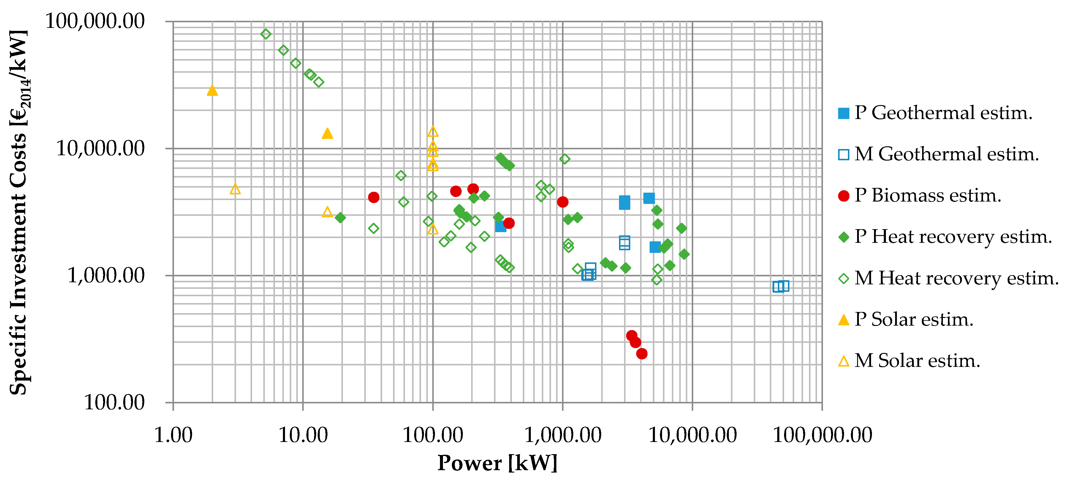
3. ORC Investment Costs: A Brief Literature Review

The body of literature on ORC systems and applications grows quickly with over 1700 references registered in the Web of Science, of which more than one third published since 2015. The importance of the economic perspective is recognized and increasingly taken along in engineering studies. The goal of this section is to give an overview of this ORC cost estimation literature. At the basis of financial-economic project analyses are the annual cash flows, composed of the capital investment and annual expenses and revenues. The capital investment is the one-time cost occurring at the beginning of the project. It includes the costs directly associated with the system (equipment, materials, labor etc. required for the equipment and the installation thereof), indirect costs (engineering, construction costs and contingencies) and other outlays (such as startup costs, working capital, etc.) [14]. At the core of an ORC project’s capital investment are the components of the ORC module itself: evaporator, expander and generator, condenser and pump. The costs for integration of the ORC module into an existing plant (e.g., for heat recovery applications) or with the equipment necessary for the system’s fuel supply vary according to the type of application. The annual expenses for ORC projects depend on the type of application and the location, but are generally of lesser importance than the investment costs. Thus, insight in the investments costs is essential to evaluate the financial feasibility of an ORC system.

Reviewing the literature reveals a variety of approaches used to evaluate ORC investment costs. Some assume a value for the ORC costs (such as [20,21,22,23,24,25,26]). However representative the assumptions and insightful the analyses, these cost figures ought not to be confused with real costs. Only very few publications provide insight into the costs of actual ORC systems (e.g., [27,28,29]). Others estimate the costs through extrapolation from known costs of components or other ORC systems or via professional cost estimators (e.g., [30,31]). An increasing amount of researchers estimate the costs of components based on equipment correlations, using either percentages ([32]) or multiplication factors ([33,34,35]) to estimate the total project costs based on the module/equipment costs. Techno-economic ([22,36,37,38,39,40,41]) as well as thermo- or exergoeconomic ([33,42,43,44]) methods are used to simultaneously analyze technical and economic aspects and tradeoffs.

Figure 1 displays a review of published data on estimated ORC investment costs. The specific investment costs (SIC) are presented as a function of capacity, plotted on a log-log scale for better representation. Within the scope of this paper, only papers that estimate ORC investment costs have been included. The following selection criteria were applied: (a) the paper performs a bottom-up estimate of ORC costs, using various techniques; (b) the power output of the ORC system is given and (c) the paper presents the resulting SIC or the total investment costs of the ORC system. This implies that Figure 1 includes no real ORC costs and that cost estimates with incomplete information could not be incorporated. The data has been categorized according to the scope of the system and the heat source. The scope refers to either an ORC module (M), which comprises only the essential components of the ORC itself without integration or installation, or an ORC project (P), including all expenses needed to integrate and install the ORC module into an existing plant or with the fuel conversion equipment. The heat sources are classified into the four groups geothermal, biomass, heat recovery, and solar. To allow for comparison, the costs are converted to euros and updated to 2014 values, using the Chemical Engineering Plant Cost Index (CEPCI). Figure 1 plots the results; suggesting decreasing SIC for increasing power output. These findings are in line with the trend reported by Quoilin et al. [45]. Scattering of the data for similar power outputs is due to different ORC designs, system delineations and estimation approaches. Solar ORC systems are most reported for smaller capacities, whereas geothermal systems are commonly larger scaled. The solar ORCs tend to have higher SICs, with an average of 21 k€₂₀₁₄/kW for the projects and 7.4 k€₂₀₁₄/kW for the modules. The estimated geothermal ORCs have an average SIC of 3156 €₂₀₁₄/kW for complete projects and 1149 €₂₀₁₄/kW for modules. The heat recovery ORC systems are more represented in the middle range, with estimated module costs around 2781 €₂₀₁₄/kW (Average calculated excluding the micro-scale diesel engine recovery ORC systems of Yang et al. [46]. Including these gives an average heat recovery module SIC of 12,149 €₂₀₁₄/kW.) and averaging project costs of 3414 €₂₀₁₄/kW. Note that the lower costs for modules than for projects are the result of averaging, but the result is in line with the finding that there are less distinct differences between module and project costs. No biomass modules are included in the data, but biomass projects are estimated in the same order of magnitude (3054 €₂₀₁₄/kW) as heat recovery systems. Recall that all the values in the graph and these averages are the result of estimates, where different estimations methods and scopes are used. These do not necessarily reflect real ORC system costs and should not be generalized as such.

Figure 1 contains only those references for which information about both the investment costs and the power output was given. Other valuable contributions are made by, for instance, Quoilin et al. [71] who perform a thermo-economic optimization of ORCs for waste heat recovery. They obtain SIC values between 2136 and 4260 €/kW, depending on the fluid operated, for small scale (<5 W_net) systems. An important conclusion from their work is that the operating point yielding maximum power does not coincide with that of minimal SIC. Similarly, Imran et al. [72] utilize thermo-economic optimization to compare cycle setups. The SIC values are in the range of 3274 to 4155 €/kW for the basic ORC, 3453 to 4571 €/kW for the single stage regenerative ORC and 3739–4960 €/kW for the double stage regenerative ORC, depending on the working fluid operated. Unfortunately no indication was given on the power range. Walraven et al. [73] investigate air-cooled geothermal ORC systems. No exact specific investment costs numbers are presented, but the impact of various factors, such as brine inlet and outlet temperatures, pressure levels, electricity prices, discount rates and electricity price evolutions, on the economics of the ORC project are demonstrated. Heberle and Brüggemann [34] perform a thermo-economic evaluation of various zeotropic mixtures for geothermal ORC systems, with SICs between 3076 and 4882 €₂₀₁₄/kW. Other studies could not be included in Figure 1 because the economic values are expressed in €/kWh rather that €/kW, such as in Meinel et al. [74] who perform a considerate comparison of architecture designs at various sizes. The results were calculated for heat sources of 0.5 MWth, 1 MWth and 5 MWth.

The references in Figure 1 all concern estimates of ORC costs; reporting on real ORC costs remains rather scarce. For instance, Leslie et al. [75] discuss the findings of a 5.5 MW ORC system applied for heat recovery from a gas turbine driving a natural gas pipeline compressor. The system was monitored extensively for one year, and the capital costs of the system constitute approximately 2500 €/kW. A 400 kW biomass ORC combined heat and power system installed in 1999 in Admont, Austria had an investment cost of about 3.2 million € [27]. The relatively high investment costs are due to the fact that this was the first biomass ORC power plant in the European Union. In 2009, prices for biomass fueled ORC systems are published in the range of 4500 €/kW for an 1803 kW system to 10,200 €/kW for a 345 kW system [28]. A heat recovery ORC plant installed in Adana, Turkey had an investment cost of $ 500,000 for 260.4 kW capacity, but the installation date is unknown [29].

4. Comparing the Estimated and Actual Costs of a Heat Recovery ORC System

This section presents the results of various cost estimation approaches to give a perspective on their methodology and accuracy. First of all, the investment costs of an actual heat recovery case are discussed. Then, the costs of this case study are estimated using both the costs of other ORC systems as well as the technical parameters of the case study itself.

4.1. Case Study: ORC for Industrial Heat Recovery

The ORC system was installed in 2013 in Flanders, Belgium to recover excess heat from an industrial plant. The excess heat is a low-medium temperature (range 150–250 °C) flue gas stream from an industrial kiln. The ORC module was integrated into the plant using an intermediate thermal oil circuit including a flue gas heat exchanger. The ORC unit itself has a gross power output of 375 kW and is composed of a centrifugal pump, a one-step radial expander and a generator. The evaporator is a plate heat exchanger and condensation occurs air-cooled. The project has a SIC of 4216 €₂₀₁₃/kW_gr, including integration (oil circuit, piping …) and installation (delivery, construction and project management). Figure 2 displays the partitioning of the capital costs. A major share of total costs stems from the ORC module itself, which includes the pump, expander and generator. The intermediate thermal oil circuit represents about 11% of total investment costs.

4.2. Using Cost Data of Other Systems: The Capacity Exponent Ratio Method

Using the capacity exponent ratio method, the costs of a piece of equipment or a complete project are estimated based on knowledge about the costs of a similar system from a different capacity or scale. For instance, Ghirardo et al. [58] investigate the options to recover heat from onboard fuel cell systems, including an ORC system. The reference ORC module costs € 1,675,000 for 1115 kW output, including an intermediate thermal oil system the total investment costs of the reference plant are calculated as € 2,345,000. Using an exponent of 0.867, the capital investment of the 35 kW system is estimated at € 117,000: ${\mathrm{c}}_{\mathrm{a}}= {\mathrm{c}}_{\mathrm{b}}{\left(\frac{{\mathrm{A}}_{\mathrm{a}}}{{\mathrm{A}}_{\mathrm{b}}}\right)}^{\mathrm{n}}=\mathrm{2,345,000}{\left(\frac{{\mathrm{A}}_{\mathrm{a}}}{1115}\right)}^{0.876}=€ \mathrm{117,000}$. Unfortunately, there is no information on the time frame in which the reference price is collected.

Several questions arise when performing a cost estimate with the Capacity Exponent Ratio. First of all, which ORC system is best to use as reference case? The most appropriate to use is a system with similar characteristics, but the available information on real ORC costs is scarce. A possible reference case for the study in this paper is given by for instance Forni et al. [57], who give insight into the feasibility of potential example cases based on cost data from an experienced manufacturer. Alternatively, David et al. [56] discuss two potential heat recovery case studies. The costs of the system are roughly gauged using prices of existing ORC modules and estimated additional costs for integration and installation. For the steel mill project, two ORC units would be needed to obtain 250 kW_gr output, at a cost of 500 €/kW_e for the units and 1080 €/kW for the complete project. A third option is a budget offer made to the City of Unalaska in 2012, which states a price of k$ 185 for a 50 kW unit, to be used for heat recovery [76]. The complete project, including labor and other project contingencies, is quoted at k$ 1889 [76]. Finally, a 5.5 MW heat recovery demonstration project installed in 2006 in the USA had a cost of 2500 $/kW [75,77]. Besides a reference case, the Capacity Exponent Ratio method requires a suitable exponent for the scaling. The commonly derived exponent for the chemical engineering industry is 0.6; Ghirardo et al. [58] use 0.867. Due to lack of sufficient data to calculate an exponent for ORC heat recovery systems specifically, the standard exponent of 0.6 is used for this analysis. The results of the cost extrapolation are displayed in

Table 2. Cost estimation using the capacity exponent ratio method.

No.	Reference Case	Reference Gross Power (kW)	Reference Module SIC	Reference Project SIC	Estimated Module SIC (€2013/kW)	Estimated Project SIC (€2013/kW)
1	[57]	1100	1818 €2012/kW	2818 €2012/kW	2796	4334
2	[57]	1300	1154 €2012/kW	2923 €2012/kW	1897	4806
3	[57]	5300	943 €2012/kW	3321 €2012/kW	2721	9579
4	[57]	5400	1148 €2012/kW	2593 €2012/kW	3337	7535
5	[57]	160	2594 €2011/kW	3375 €2011/kW	1845	2401
6	[57]	250	2080 €2011/kW	4320 €2011/kW	1769	3673
7	[76]	50	3700 USD2012/kW	-	1653	-
8	[76]	150	-	12,596 USD2012/kW	-	8731
9	[75,77]	5500	-	2500 USD2006/kW	-	7319

, using the investment costs available in each of the discussed potential references [55,57,75,76,77].

The project costs are calculated for information purposes, but because the integration requirements are so different per case these cannot be compared to the costs of the case study. The module costs of the 375 kW case study are estimated between 1653 and 3337 €₂₀₁₃/kW, with an average of 2288 €₂₀₁₃/kW. This variation can have various origins, such as manufacturer experience or margins, inclusion of freight or engineering costs or not. Comparing these results to the costs of the case study, we would have expected case no. 6 to yield good results since the heat recovery setup and the suggested ORC module are similar to that of the case study. Similarly, case no. 7 concerns an actual budget quote and was expected to be representative. Although case no. 6 and 7 lead to mutually similar results, there is a large deviation with the 3280 €₂₀₁₃/kW of the real case. This, again, can be due to the specific sales circumstances, due to the fact that the estimated costs do not take account of some essential costs or perhaps due to overpricing of the real case. Because the detailed cost decomposition of the reference cases is not sufficiently known, it is not possible to obtain very accurate estimates or comparisons. Thus, the capacity exponent ratio method can be used only for order-of-magnitude or study estimates [18]. The accuracy of this estimation method for ORC investments may increase as more and sufficiently detailed knowledge about actual ORC systems is published.

4.3. Using Technical Parameters of the System: Factorial Estimation Techniques

Factorial costs estimation techniques use information about the technical details of the designed system itself, rather than cost information of other but similar systems. Again, the purchased equipment costs form the basis of the total investment costs, but these are now estimated using cost correlations for all major equipment items. The total investment costs are then derived from these purchased equipment costs, using either multiplication factors or percentages.

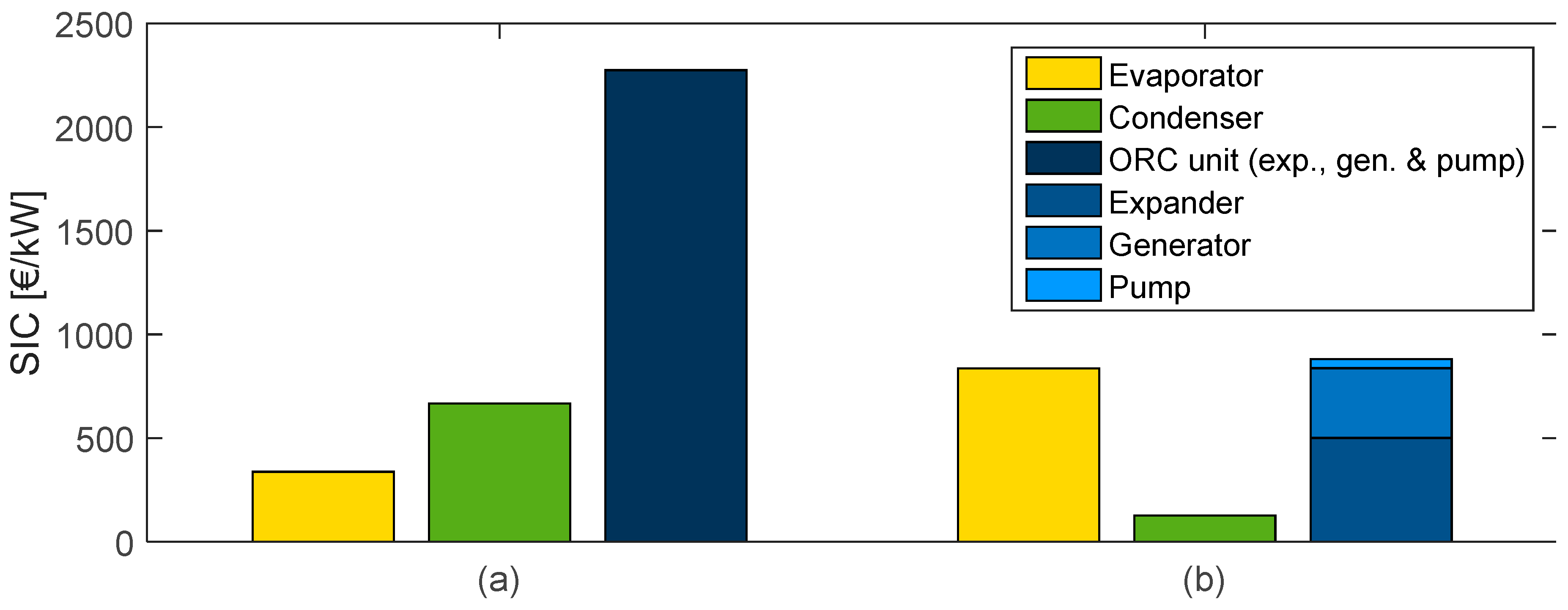
4.3.1. Estimating the Purchased Equipment Costs

The costs of the major equipment items are commonly estimated from publicly available equipment cost correlations, which have been established for a large number of commonly used industrial equipment. For ORC systems, the major equipment items are the basic components: the evaporator, expander and generator, condenser and pump. Because there is little information about the component costs of actual ORC systems, most researchers use publicly available correlations for standard equipment items. For instance, Lee et al. [62] were early to use component correlations to estimate the costs of an ORC heat recovery system. Quoilin et al. [71] combine correlations from literature [14] with self-derived ones. Walraven et al. [49] combine correlations from various sources [16,17,78] for their analysis. Desai and Bandyopadhyay [79] combine correlations from various ORC research papers. An increasing number of researchers utilize the correlations from Turton et al. [13] for ORC cost estimation (e.g., [36,46,47,48,50]).

A similar procedure is performed to estimate the purchased equipment costs of the case study discussed in this paper. Knowing the technical parameters of the system, the component costs are estimated from publicly available correlations. The evaporator, expander and pump costs are calculated from the correlations of Turton et al. [13], of the form

$${\lg }_{10}{\mathrm{C}}_{\mathrm{p}}^0={\mathrm{K}}_1+{\mathrm{K}}_2{\log }_{10}\left(\mathrm{A}\right)+{\mathrm{K}}_3{[{\log }_{10}\left(\mathrm{A}\right)]}^2$$

with ${\mathrm{C}}_{\mathrm{p}}^0$ being the purchased equipment costs at ambient pressure and using carbon steel, $\mathrm{A}$ the equipment attribute and ${\mathrm{K}}_1$, ${\mathrm{K}}_2$ and ${\mathrm{K}}_3$ the coefficients determined for the type of equipment [13]. The condenser fan costs are estimated with a correlation from Smith [16] and for the generator the function available in Toffolo et al. [48] is applied. The coefficients and correlations are summarized in

Table 3. Coefficients and correlations for estimation of the purchased equipment costs.

Component	Coefficients and Correlations			Reference
Evaporator	${\mathrm{K}}_1=4.6656$	${\mathrm{K}}_2=-0.1557$	${\mathrm{K}}_3=0.1547$	[13]
Expander	${\mathrm{K}}_1=2.2476$	${\mathrm{K}}_2=1.4965$	${\mathrm{K}}_3=-0.1618$	[13]
Pump	${\mathrm{K}}_1=3.3892$	${\mathrm{K}}_2=0.0536$	${\mathrm{K}}_3=0.1538$	[13]
Condenser	${\mathrm{C}}_{\mathrm{p}}^0= \mathrm{12,300}\times {\left(\frac{\mathrm{Q}}{50}\right)}^{0.76}$ with Q in kW			[16]
Generator	${\mathrm{C}}_{\mathrm{p}}^0=\mathrm{1,850,000}\times {\left(\frac{\mathrm{P}}{\mathrm{11,800}}\right)}^{0.94}$ with P in kW			[48]

. All estimates are converted to 2013 Euros to allow for comparison with the actual costs of the case study. The correlations from Turton et al. [13] yield values in USD₂₀₀₁. These are converted to Euros using a 1.1162 exchange rate (average 2001) and updated to 2013 using the Chemical Engineering Plant Cost Index (CEPCI), with CEPCI₂₀₀₁ and CEPCI₂₀₁₃ values of 397 and 587.3 respectively. The results obtained from Smith [16] are converted from USD_Jan,2000 to €₂₀₁₃ using an exchange rate of 0.9857 (average Jan 2000) and CEPCI₂₀₀₀ equal to 394.1. The correlation from Toffolo et al. [48] is in Euros and was first published in 1993, so a CEPCI₁₉₉₃ of 359.2 was used.

The results of the cost estimate are presented in

Table 4. Factorial estimation of the purchased equipment costs.

Component	${\mathbf{C}}_{\mathbf{p}}^{\mathbf{0}}$ (€2013)
Evaporator	313,539.06
Expander	187,773.74
Pump	16,370.16
Condenser	47,325.76
Generator	126,282.44
Total	691,291.16
Specific investment costs (€2013/kWgr)	1843.44

. The module costs of the case study, composed of the components but without integration costs, amount 3280 €₂₀₁₃/kW. The SIC are estimated at 1843 €₂₀₁₃/kW when only the essential ORC components are considered. These costs are often interpreted as the costs for the ORC module, but are significantly lower (−44%) than the actual figure. However, this comparison may not be completely justified because part of this difference could be due to the fact that the real module costs already include additional costs such as freight, engineering or instrumentation. Estimating the purchased equipment costs as the ORC module costs can give a first proxy but will likely underestimate the real detailed composition of the ORC module.

A comparison of the real (a) and the estimated (b) component costs for the case study is presented in Figure 3. The ORC module is composed of the evaporator, condenser and the ORC unit which includes the expander, generator and pump. These are the purchased equipment costs excluding integration and other additional costs. Figure 3 demonstrates not only the difference between the real and the estimated costs, but also highlights the significant divergence of the cost distributions. The expectation was that there could be a deviation in the absolute values, but that the cost distribution would be more representative. Nevertheless, there are large discrepancies. For instance, the evaporator constitutes only 10% of the real purchased equipment costs but is estimated at a 45% share. The ORC unit, including expander, generator and pump, represents 69% of actual purchased equipment costs but its share is estimated at 47%.

4.3.2. Estimating the Total Investment Costs: Multiplication Factors

The utilization of a multiplication factor to account for direct (purchased equipment, piping, instrumentation and controls …) and indirect (engineering and supervision, construction, contingencies) costs is attributed to Lang. The method has been adapted several times throughout the years aiming for better, more accurate results. Also for ORC research cost estimation this technique is more often used: the total investment costs are estimated using the estimated purchased equipment costs. Some multiply the purchased equipment costs by a factor of 6.32 to obtain the total investment costs (e.g., [33,34,35]), as suggested by Bejan et al. [14]. Note that this 6.32 multiplication factor is suggested for the erection of new systems; for expansion of existing systems a factor of 4.16 is proposed [14]. Nevertheless, such a general multiplication factor fails to take account of the project specific integration requirements. The necessary piping, heat exchange or other intermediate equipment differs strongly per case, but also per type of application. For new geothermal projects the integration requirements are very likely much higher than for heat recovery projects where the base plant is already operational. Suppose the 4.16 multiplication factor, for expansion of existing systems, is used to estimate the case study’s costs. Using the estimated purchased equipment costs of 1843 €₂₀₁₃/kW as a basis, this would give a total investment cost of 7667 €₂₀₁₃/kW. This is a deviation of 82% from the actual 4216 €₂₀₁₃/kW.

Other factorial approaches are applied by for instance Huang et al. [38,39], who use the ECLIPSE program, designed for technical, environmental and economic process analysis, to estimate the costs of the proposed biomass ORC systems. Finally, the module costing technique illustrated by Turton et al. [13] is a commonly used factorial cost estimation method based on the approach of Guthrie [13]. It is increasingly applied in ORC research (see e.g., [47,48,50,61,62,65]). This technique is suitable for preliminary estimates in the −20% to +30% accuracy range. The costs of the major purchased equipment parts are estimated based on technical characteristics, as described in Section 4.3.1 [13]. These base costs ${\mathrm{C}}_{\mathrm{p}}^0$ are multiplied with the bare module cost factor ${\mathrm{F}}_{\text{BM}}$, which accounts for operating pressures and specific materials of construction, as well as direct and indirect project expenses. This yields the bare module costs ${\mathrm{C}}_{\text{BM}}$ [13]:

$${\mathrm{C}}_{\text{BM}}={\mathrm{C}}_{\mathrm{p}}^0{\mathrm{F}}_{\text{BM}}$$

The project costs ${\mathrm{C}}_{\text{TM}}$ (referred to as the total module costs in [13]) include the integration of the plant into an existing facility. They are obtained by adapting the bare module costs with another multiplication factor:

$${\mathrm{C}}_{\text{TM}}= 1.18{\displaystyle \sum }_{i=1}^n{\mathrm{C}}_{\text{BM},\mathrm{i}}$$

where $n$ is the total amount of equipment parts [13].

This approach is applied to estimate the total project costs of the case study, starting from the purchased equipment costs estimate in Section 4.3.1. Accounting for the used materials and pressures, the direct (equipment, installation materials and labor) and indirect (freight, insurance, taxes, overhead and engineering expenses) costs associated with the project yields a specific bare module cost of 4390 €₂₀₁₃/kW. Finally, the total module costs include also contingencies and contractor fees and auxiliary facilities. They are obtained by multiplying the bare module costs with a factor 1.18 and are estimated at 5180 €₂₀₁₃/kW. The results are shown in

Table 5. Total investment costs estimation with the Module Costing Technique [13].

Component	${\mathbf{C}}_{\mathbf{p}}^{\mathbf{0}}$ (€2013)	${\mathbf{C}}_{\mathbf{B}\mathbf{M}}$ (€2013)	${\mathbf{C}}_{\mathbf{T}\mathbf{M}}$ (€2013)
Evaporator	313,539.06	680,379.76
Expander	187,773.74	657,208.08
Pump	16,370.16	53,039.31
Condenser	47,325.76	66,256.07
Generator	126,282.44	189,423.67
Total	691,291.16	1,646,306.89	1,942,642.13
Specific investment costs (€2013/kWgr)	1843.44	4390.15	5180.38

. Based on these estimates the ORC total module costs are almost three times as high as the costs of the module itself, composed of the major equipment items.

The real project costs are composed of the equipment, but also the costs for integration and installation and amount 4216 €₂₀₁₃/kW. The estimated total module costs amount 5180 €₂₀₁₃/kW, which is 23% higher. These total module costs are commonly interpreted as the total costs associated with an ORC project, including the ORC module itself and its integration into an existing plant or into the facilities for conversion of the energy source. However, these total costs have been obtained using multiplication factors that have been established based on other industrial applications. In practice, the actual requirements for integration differ per application. For this heat recovery case study, the integration involved an intermediate thermal oil circuit and associated piping. The integration costs and the costs charged by the ORC vendor to install the system amount 22% of the total project costs. For the estimate the module costs represent only 35.6% of the total, the remainder interpreted as the integration and other project costs.

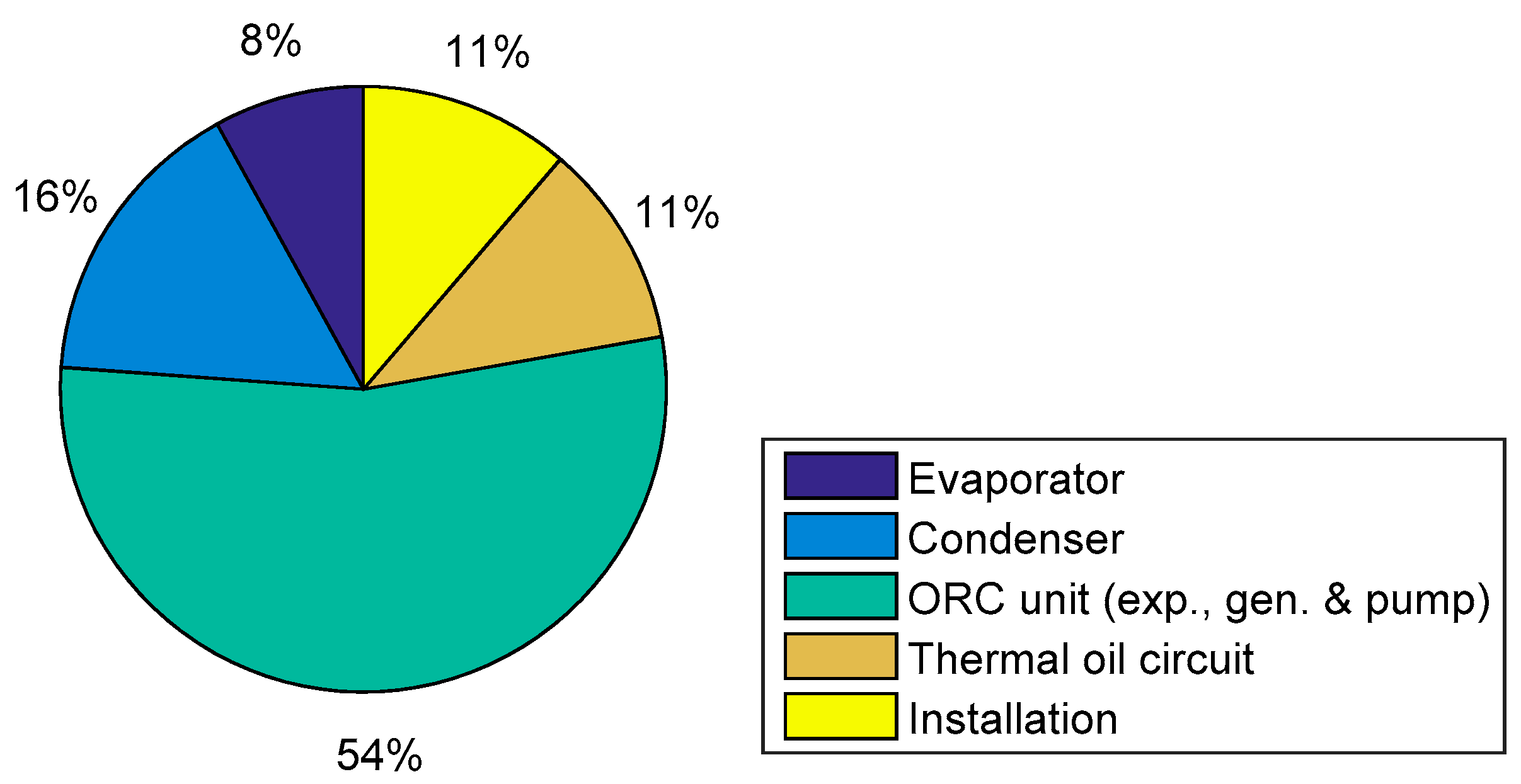
4.3.3. Estimating the Total Investment Costs: Percentages of Delivered Equipment Costs

The percentages of delivered equipment approach starts from the purchased equipment costs and calculates the other cost factors as percentages of the former. The methodology and applicable percentages are illustrated by Bejan et al. [14] and Peters et al. [18]. The applied percentages are based on the average percentages suggested by Bejan et al. [14]. Starting from the estimated purchased equipment costs of 1843 €₂₀₁₃/kW, the total investment costs are estimated as shown in

Table 6. Total investment costs estimation using percentages of delivered equipment costs.

Cost Breakdown	Percentage Range	Applied Percentage	Cost Estimate (€2013/kW)
1. Fixed-capital investment (FCI)
1.1. Direct fixed-capital investment (DFCI)
1.1.1. Onsite costs (ONSC)
Purchased-equipment cost (PEC)	15%–40% of FCI [14,18]	/	1843.44
Purchased-equipment installation	6%–14% of FCI; 20%–90% of PEC [14,18]	45% of PEC [14]	829.55
Piping	4%–17% of FCI; 3%–20% of FCI; 10%–70% of PEC	31% of PEC [14]	571.47
Instrumentation and controls	2%–12% of FCI; 2%–8% of FCI; 6%–40% of PEC	10% of PEC [14]	184.34
Electrical equipment and materials	2%–10% of FCI; 10%–15% of PEC	11% of PEC [14]	202.78
1.1.2. Offsite costs (OFSC)
Land	1%–2% of FCI; 0%–2% of FCI; 0%–10% of PEC	/	0
Civil, structural, and architectural work	5%–23% of FCI; 15%–90% of PEC	44% of PEC [14]	811.11
Service facilities	8%–30% of FCI; 30%–100% of PEC	20% of PEC [14]	368.69
Buildings	2%–18% of FCI	/	0
Yard improvements	2%–5% of FCI	/	0
Total DFCI			4811.38
1.2. Indirect Fixed-Capital Investments (IFCI)
Engineering and supervision	4%–20% of FCI [18]; 4%–21% of FCI [14]; 6%–15% of DFCI [14]; 25%–75% of PEC [14]	30% of PEC [14]	553.03
Construction costs including contractor’s profit	4%–17% of FCI [18]; 6%–22% of FCI [14]; 15% of DFCI [14]	15% of DFCI [14]	721.71
Contingencies	5%–15% of FCI [18]; 5%–20% of FCI [14]; 8%–25% of all direct and indirect costs, without legal costs [14]	10% of FCI [14]	691.60
Legal costs	1%–3% of FCI [18]	2% of FCI [14]	138.32
Total IFCI			2104.66
2. Other outlays
Startup costs	5%–12% of FCI [14]	10% of FCI [14]	691.60
Working capital	10%–20% of TCI [14]	/	0
Costs of licensing, research, and development	/	/	0
Allowance for funds used during construction (AFUDC)	/	/	0
Total capital investment			7607.65

. The resulting value of 7608 €₂₀₁₃/kW is much higher than the actual costs, but close to the 7667 €₂₀₁₃/kW obtained with the simple 4.16 factor multiplication demonstrated in Section 4.3.1. This is not surprising, since the general multiplication factors proposed by Bejan et al. [14] have been derived from this percentage approach.

5. Discussion and Conclusions

The adoption and diffusion of innovative technologies is strongly influenced by economic aspects. For ORC systems, the capital costs have a major influence on the financial feasibility of the investment project. The importance of the economic dimension is increasingly recognized and an expanding number of researchers incorporate an economic chapter in their work. Because there is still not much published information about the actual costs of ORC systems and their components, the capital costs of the proposed designs are estimated from publicly available component correlations or aggregated cost data. The aim of this paper is to provide a perspective on these cost engineering techniques and their applicability for of ORC systems.

The various methods available to estimate the capital costs of industrial equipment are concisely outlined. In case the costs of a similar piece of equipment or a similar plant are available, the required costs can simply be estimated through exponential scaling (capacity exponent ratio method). More detailed estimates use factorial estimation techniques, with cost correlations and coefficients based on experience and a larger number of reference units. However, any up-front cost estimate should be considered with respect to its expected accuracy range. Simpler methods require less effort but yield lower accuracy. High accuracies are possible with definitive and detailed estimates, but these require a far-reaching detail of plant design. Cost estimates pursued in the frame of research generally achieve accuracies in the range of order-of-magnitude, study or preliminary estimates. Subsequently, a literature review concerning the results of ORC investment cost estimates reveals a trend of decreasing specific investment costs for larger capacities. Geothermal systems tend to be larger; solar systems are mostly small and can have very high specific investment costs. The variability in estimation results stems from differing estimation approaches or scopes. Finally, the investment costs of an actual heat recovery case study are outlined and used to benchmark various cost estimation techniques. Estimating the costs via scaling of similar systems gives estimated module costs between 1653 and 3337 €₂₀₁₃/kW and applying commonly used component cost correlations yields an estimated purchased equipment cost of 1843 €₂₀₁₃/kW. The module costs of the actual system amount 3280 €₂₀₁₃/kW. Estimating the total investment costs yields 7667 €₂₀₁₃/kW when one single factor is used, 5180 €₂₀₁₃/kW when the module costing technique is applied and 7608 €₂₀₁₃/kW for estimation via the percentages of delivered equipment method. The actual total investment costs amount 4216 €₂₀₁₃/kW. Note that this analysis compares the estimated and real costs for only one case study, so the results should not be generalized. For instance, Toffolo et al. [48] perform a similar analysis and they report only a very small difference between estimated and actual costs.

There are several potential reasons for deviations between actual and estimated investment costs. First of all, capacity exponent ratio methods have expected accuracies suitable for order-of-magnitude or study estimates, factorial estimation methods such as the module costing technique are suitable for preliminary estimates. A deviation of −50% to +100% for the former and −20% to +30% for the latter is therefore not uncommon. The best results are obtained with the module costing technique, but the correlations and multiplication factors have been established for other applications. Development of correlations and multiplication factors for ORC technology in particular is likely to improve the quality of the estimates.

Second, the accuracy of factorial estimation methods depends strongly on the quality of the information that was used to establish the multiplication factors. Because there is little public information about the actual costs of ORC systems and their components, approximations from other industrial fields are used. The accuracies of ORC cost estimates could increase as more technology-specific cost information becomes available.

Additional inaccuracies and uncertainties stem from treatment of costs over time periods. Extrapolation of costs over large periods of time decreases the accuracy of the results. Most of the open-source correlations available in text books are at least nine years old and thus provide less accurate results. Moreover, some of these references refer back to original factors and correlations published by Guthrie in 1969 or 1974 and updated with few recent data points or using cost indices. This makes these correlations less reliable. Also, the choice of indicator for cost escalation and local conditions may have an influence and create additional deviations.

Furthermore, it is important to acknowledge the difference between costs and prices. Costs reflect the amount that is required to produce a certain item; the price is the amount you pay to purchase it. The costs associated with producing an ORC system will thus differ from the price paid to acquire that system. Many correlations used to estimate costs are obtained using vendor prices. In cases where the ORC developer would purchase most equipment instead of developing, it this is not a problem. For innovative system designs (e.g., expanders) this method would be less suitable.

Finally, for the specific case of ORC projects the costs depend strongly on the type of application. Whereas the estimated “total module costs” are often interpreted as the complete ORC project costs, these are all using the same multiplication factors and fail to take account of the diversity of integration requirements. ORC projects using biomass, geothermal, solar or excess heat have different integration requirements and corresponding costs. These multiplication factors have been established for applications in mostly the chemical engineering industry, so their use for other industries may be less reliable.

These findings have several implications. First and foremost, estimated cost figures should be accompanied by accuracy ranges and a discussion on the reliability of the used methods. This to avoid misinterpretation of the validity of the results. The correlations that are currently available are useful to mutually compare various system designs, where the proportional comparison is more important than the exact outcomes. The results are relative rather than absolute. Secondly, proper delineation of the scope of the investigation is key to enhance usability and comparability of the results. This relates to defining whether the module or the project costs are considered, and which cost aspects are included or not, as well as providing a date stamp for any cost figure. Finally, estimating the total investment costs of an ORC project by extrapolation or multiplication does not take into account the case-specific integration requirements. These are more difficult to estimate because of their diversity, but could be approximated when there are sufficient real data to identify average multiplication factors per application type. Estimating the purchased equipment costs is essential to investigate the ORC module costs, but the result can be an underestimation of the actual figure.

References

1. Chen, H.; Goswami, D.Y.; Stefanakos, E.K. A review of thermodynamic cycles and working fluids for the conversion of low-grade heat. Renew. Sustain. Energy Rev. 2010, 14, 3059–3067. [Google Scholar] [CrossRef]
2. Lecompte, S.; Huisseune, H.; van den Broek, M.; Vanslambrouck, B.; De Paepe, M. Review of organic Rankine cycle (ORC) architectures for waste heat recovery. Renew. Sustain. Energy Rev. 2015, 47, 448–461. [Google Scholar] [CrossRef]
3. Lakew, A.A.; Bolland, O. Working fluids for low-temperature heat source. Appl. Therm. Eng. 2010, 30, 1262–1268. [Google Scholar] [CrossRef]
4. Hung, T.-C. Waste heat recovery of organic Rankine cycle using dry fluids. Energy Convers. Manag. 2001, 42, 539–553. [Google Scholar] [CrossRef]
5. Brown, J.S.; Brignoli, R.; Quine, T. Parametric investigation of working fluids for organic Rankine cycle applications. Appl. Therm. Eng. 2015, 90, 64–74. [Google Scholar] [CrossRef]
6. Declaye, S.; Quoilin, S.; Guillaume, L.; Lemort, V. Experimental study on an open-drive scroll expander integrated into an ORC (Organic Rankine Cycle) system with R245fa as working fluid. Energy 2013, 55, 173–183. [Google Scholar] [CrossRef]
7. Papes, I.; Degroote, J.; Vierendeels, J. New insights in twin screw expander performance for small scale ORC systems from 3D CFD analysis. Appl. Therm. Eng. 2015, 91, 535–546. [Google Scholar] [CrossRef]
8. Jaffe, A.B.; Stavins, R.N. The energy paradox and the diffusion of conservation technology. Resour. Energy Econ. 1994, 16, 91–122. [Google Scholar] [CrossRef]
9. Rogers, E.M. Diffusion of Innovations, 5th ed.; Free Press: New York, NY, USA, 2003. [Google Scholar]
10. Jaffe, A.B.; Newell, R.G.; Stavins, R.N. Economics of Energy Efficiency. Encycl. Energy 2004, 2, 79–90. [Google Scholar]
11. Lemmens, S. A perspective on costs and cost estimation techniques for organic Rankine cycle systems. In Proceedings of the 3rd International Seminar on ORC Power Systems (ASME ORC 2015), Brussels, Belgium, 12–14 October 2015.
12. AACE International. Recommended Practice No. 18R-97. Cost Estimate Classification System—As Applied in Engineering, Procurement, and Construction for the Process Industries. TCM Framework: 7.3—Cost Estimating and Budgeting; AACE International: Morgantown, WV, USA, 2005; p. 10. [Google Scholar]
13. Turton, R.; Bailie, R.C.; Whiting, W.B.; Shaeiwitz, J.A.; Bhattacharyya, D. Analysis, Synthesis, and Design of Chemical Processes, 4th ed.; Pearson Education International: Upper Saddle River, NJ, USA, 2013. [Google Scholar]
14. Bejan, A.; Tsatsaronis, G.; Moran, M. Thermal Design and Optimization; Wiley & Sons: New York, NY, USA, 1996; p. 542. [Google Scholar]
15. Couper, J.R.; Penney, R.W.; Fair, J.R.; Walas, S.M. Chemical Process Equipment: Selection and Design, 3rd ed.; Butterworth-Heinemann: Oxford, UK, 2012. [Google Scholar]
16. Smith, R. Chemical Process Design and Integration; John Wiley & Sons, Ltd.: West Sussex, UK, 2005. [Google Scholar]
17. Towler, G.; Sinnot, R. Chemical Egineering Design: Principles, Practice and Economics of Plant and Process Design; Butterworth-Heinemann: Oxford, UK, 2008. [Google Scholar]
18. Peters, M.S.; Timmerhaus, K.D.; West, R.E. Plant Design and Economics for Chemical Engineers, 5th ed.; McGraw-Hill: New York, NY, USA, 2004. [Google Scholar]
19. Jelen, F.C.; Black, J.H. Cost and Optimization Engineering, 2nd ed.; McGraw-Hill, Inc.: New York, NY, USA, 1983. [Google Scholar]
20. Yari, M.; Mahmoudi, S.M.S. A thermodynamic study of waste heat recovery from GT-MHR using organic Rankine cycles. Heat Mass Transf. 2010, 47, 181–196. [Google Scholar] [CrossRef]
21. Arvay, P.; Muller, M.R.; Ramdeen, V.; Cunningham, G. Economic Implementation of the Organic Rankine Cycle in Industry. In Proceedings of the 2011 ACEEE Summer Study on Energy Efficiency in Industry, Niagara Falls, NY, USA, 26–29 July 2011.
22. Algieri, A.; Morrone, P. Techno-economic Analysis of Biomass-fired ORC Systems for Single-family Combined Heat and Power (CHP) Applications. Energy Procedia 2014, 45, 1285–1294. [Google Scholar] [CrossRef]
23. Arslan, O.; Ozgur, M.A.; Kose, R. Electricity Generation Ability of the Simav Geothermal Field: A Technoeconomic Approach. Energy Sources Part A 2012, 34, 1130–1144. [Google Scholar] [CrossRef]
24. Arslan, O.; Yetik, O. ANN based optimization of supercritical ORC-Binary geothermal power plant: Simav case study. Appl. Therm. Eng. 2011, 31, 3922–3928. [Google Scholar] [CrossRef]
25. Bruno, J.C.; López-Villada, J.; Letelier, E.; Romera, S.; Coronas, A. Modelling and optimisation of solar organic rankine cycle engines for reverse osmosis desalination. Appl. Therm. Eng. 2008, 28, 2212–2226. [Google Scholar] [CrossRef]
26. Kosmadakis, G.; Manolakos, D.; Papadakis, G. Simulation and economic analysis of a CPV/thermal system coupled with an organic Rankine cycle for increased power generation. Sol. Energy 2011, 85, 308–324. [Google Scholar] [CrossRef]
27. STIA—Holzindustrie Ges.m.b.H. Biomass Fired CHP Plant Based on an ORC Cycle; Project: ORC-STIA-Admont; STIA−Holzindustria Ges.m.b.H. in Cooperation with BIOS-Bioenergy Systems: Admont, Austria, 2001; pp. 1–12. [Google Scholar]
28. Duvia, A.; Guercio, A.; di Schio, C.R. Technical and Economic Aspects of Biomass Fuelled CHP Plants Based on ORC Turbogenerators Feeding Existing District Heating Networks; Turboden: Brescia, Italy, 2009. [Google Scholar]
29. Tumen Ozdil, N.F.; Segmen, M.R. Investigation of the effect of the water phase in the evaporator inlet on economic performance for an Organic Rankine Cycle (ORC) based on industrial data. Appl. Therm. Eng. 2016, 100, 1042–1051. [Google Scholar] [CrossRef]
30. Campos Rodríguez, C.E.; Escobar Palacio, J.C.; Venturini, O.J.; Silva Lora, E.E.; Cobas, V.M.; Marques dos Santos, D.; Lofrano Dotto, F.R.; Gialluca, V. Exergetic and economic comparison of ORC and Kalina cycle for low temperature enhanced geothermal system in Brazil. Appl. Therm. Eng. 2013, 52, 109–119. [Google Scholar] [CrossRef]
31. Uris, M.; Linares, J.I.; Arenas, E. Techno-economic feasibility assessment of a biomass cogeneration plant based on an Organic Rankine Cycle. Renew. Energy 2014, 66, 707–713. [Google Scholar] [CrossRef]
32. Di Maria, F.; Micale, C. Exergetic and Economic Analysis of Energy Recovery from the Exhaust Air of Organic Waste Aerobic Bioconversion by Organic Rankine Cycle. Energy Procedia 2015, 81, 272–281. [Google Scholar] [CrossRef]
33. Heberle, F.; Bassermann, P.; Preißinger, M.; Brüggemann, D. Exergoeconomic optimization of an Organic Rankine Cycle for low-temperature geothermal heat sources. Int. J. Thermodyn. 2012, 15. [Google Scholar] [CrossRef]
34. Heberle, F.; Brüggemann, D. Thermo-Economic Evaluation of Organic Rankine Cycles for Geothermal Power Generation Using Zeotropic Mixtures. Energies 2015, 8, 2097–2124. [Google Scholar] [CrossRef]
35. Heberle, F.; Brüggemann, D. Thermo-Economic Analysis of Zeotropic Mixtures and Pure Working Fluids in Organic Rankine Cycles for Waste Heat Recovery. Energies 2016, 9, 226. [Google Scholar] [CrossRef]
36. Yu, G.; Shu, G.; Tian, H.; Wei, H.; Liang, X. Multi-approach evaluations of a cascade-Organic Rankine Cycle (C-ORC) system driven by diesel engine waste heat: Part B-techno-economic evaluations. Energy Convers. Manag. 2016, 108, 596–608. [Google Scholar] [CrossRef]
37. Astolfi, M.; Romano, M.C.; Bombarda, P.; Macchi, E. Binary ORC (Organic Rankine Cycles) power plants for the exploitation of medium–low temperature geothermal sources—Part B: Techno-economic optimization. Energy 2014, 66, 435–446. [Google Scholar] [CrossRef]
38. Huang, Y.; McIlveen-Wright, D.R.; Rezvani, S.; Huang, M.J.; Wang, Y.D.; Roskilly, A.P.; Hewitt, N.J. Comparative techno-economic analysis of biomass fuelled combined heat and power for commercial buildings. Appl. Energy 2013, 112, 518–525. [Google Scholar] [CrossRef]
39. Huang, Y.; Wang, Y.D.; Rezvani, S.; McIlveen-Wright, D.R.; Anderson, M.; Mondol, J.; Zacharopoulos, A.; Hewitt, N.J. A techno-economic assessment of biomass fuelled trigeneration system integrated with organic Rankine cycle. Appl. Therm. Eng. 2013, 53, 325–331. [Google Scholar] [CrossRef]
40. Law, R.; Harvey, A.; Reay, D. Techno-economic comparison of a high-temperature heat pump and an organic Rankine cycle machine for low-grade waste heat recovery in UK industry. Int. J. Low-Carbon Technol. 2013, 8, i47–i54. [Google Scholar] [CrossRef]
41. Rentizelas, A.; Karellas, S.; Kakaras, E.; Tatsiopoulos, I. Comparative techno-economic analysis of ORC and gasification for bioenergy applications. Energy Convers. Manag. 2009, 50, 674–681. [Google Scholar] [CrossRef] [Green Version]
42. Zare, V. A comparative exergoeconomic analysis of different ORC configurations for binary geothermal power plants. Energy Convers. Manag. 2015, 105, 127–138. [Google Scholar] [CrossRef]
43. Khaljani, M.; Saray, R.K.; Bahlouli, K. Comprehensive analysis of energy, exergy and exergo-economic of cogeneration of heat and power in a combined gas turbine and organic Rankine cycle. Energy Convers. Manag. 2015, 97, 154–165. [Google Scholar] [CrossRef]
44. Darvish, K.; Ehyaei, M.; Atabi, F.; Rosen, M. Selection of Optimum Working Fluid for Organic Rankine Cycles by Exergy and Exergy-Economic Analyses. Sustainability 2015, 7, 15362–15383. [Google Scholar] [CrossRef]
45. Quoilin, S.; van den Broek, M.; Declaye, S.; Dewallef, P.; Lemort, V. Techno-economic survey of Organic Rankine Cycle (ORC) systems. Renew. Sustain. Energy Rev. 2013, 22, 168–186. [Google Scholar] [CrossRef]
46. Yang, F.; Zhang, H.; Song, S.; Bei, C.; Wang, H.; Wang, E. Thermoeconomic multi-objective optimization of an organic Rankine cycle for exhaust waste heat recovery of a diesel engine. Energy 2015, 93, 2208–2228. [Google Scholar] [CrossRef]
47. Lazzaretto, A.; Toffolo, A.; Manente, G.; Rossi, N.; Paci, M. Cost evaluation of organic Rankine cycles for low temperature geothermal sources. In Proceedings of the 24th International Conference on Efficiency, Cost, Optimization, Simulation and Environmental Impact of Energy Systems, Novi Sad, Serbia, 4–7 July 2011.
48. Toffolo, A.; Lazzaretto, A.; Manente, G.; Paci, M. A multi-criteria approach for the optimal selection of working fluid and design parameters in Organic Rankine Cycle systems. Appl. Energy 2014, 121, 219–232. [Google Scholar] [CrossRef]
49. Walraven, D.; Laenen, B.; D’haeseleer, W. Minimizing the levelized cost of electricity production from low-temperature geothermal heat sources with ORCs: Water or air cooled? Appl. Energy 2015, 142, 144–153. [Google Scholar] [CrossRef]
50. Yang, M.-H.; Yeh, R.-H. Economic performances optimization of an organic Rankine cycle system with lower global warming potential working fluids in geothermal application. Renew. Energy 2016, 85, 1201–1213. [Google Scholar] [CrossRef]
51. Barber, R.E. Current costs of solar powered organic Rankine cycle engines. Sol. Energy 1978, 20, 1–6. [Google Scholar] [CrossRef]
52. Georges, E.; Declaye, S.; Dumont, O.; Quoilin, S.; Lemort, V. Design of a small-scale organic Rankine cycle engine used in a solar power plant. Int. J. Low-Carbon Technol. 2013, 8, i34–i41. [Google Scholar] [CrossRef]
53. Manolakos, D.; Mohamed, E.S.; Karagiannis, I.; Papadakis, G. Technical and economic comparison between PV-RO system and RO-Solar Rankine system. Case study: Thirasia island. Desalination 2008, 221, 37–46. [Google Scholar] [CrossRef]
54. Kosmadakis, G.; Manolakos, D.; Kyritsis, G.; Papadakis, G. Economic assessment of a two-stage solar organic Rankine cycle for reverse osmosis desalination. Renew. Energy 2009, 34, 1579–1586. [Google Scholar] [CrossRef]
55. Amini, A.; Mirkhani, N.; Pakjesm Pourfard, P.; Asjaee, M.; Khodkar, M.A. Thermo-economic optimization of low-grade waste heat recovery in Yazd combined-cycle power plant (Iran) by a CO2 transcritical Rankine cycle. Energy 2015, 86, 74–84. [Google Scholar] [CrossRef]
56. David, G.; Michel, F.; Sanchez, L. Waste heat recovery projects using Organic Rankine Cycle technology—Examples of biogas engines and steel mills applications. In Proceedings of the World Engineers’ Convention, Geneva, Switzerland, 4–9 September 2011; pp. 1–11.
57. Forni, D.; Vaccari, V.; Di Santo, D.; Rossetti, N.; Baresi, M. Heat recovery for electricity generation in industry. In Proceedings of the European Council for an Energy Efficient Economy 2012 Summer Study on Energy Efficiency in Industry, Arnhem, The Netherlands, 11–14 September 2012.
58. Ghirardo, F.; Santin, M.; Traverso, M.; Masssardo, A. Heat recovery options for onboard fuel cell systems. Int. J. Hydrog. Energy 2011, 36, 8134–8142. [Google Scholar] [CrossRef]
59. Kwak, D.-H.; Binns, M.; Kim, J.-K. Integrated design and optimization of technologies for utilizing low grade heat in process industries. Appl. Energy 2014, 131, 307–322. [Google Scholar] [CrossRef]
60. Lecompte, S.; Huisseune, H.; van den Broek, M.; De Schampheleire, S.; De Paepe, M. Part load based thermo-economic optimization of the Organic Rankine Cycle (ORC) applied to a combined heat and power (CHP) system. Appl. Energy 2013, 111, 871–881. [Google Scholar] [CrossRef]
61. Lecompte, S.; Lazova, M.; van den Broek, M.; De Paepe, M. Multi-objective optimization of a low-temperature transcritical organic Rankine cycle for waste heat recovery. In Proceedings of the 10th International Conference on Heat Transfer, Fluid Mechanics and Thermodynamics (HEFAT2014), Orlando, FL, USA, 14–16 July 2014.
62. Lecompte, S.; Lemmens, S.; Huisseune, H.; van den Broek, M.; De Paepe, M. Multi-Objective Thermo-Economic Optimization Strategy for ORCs Applied to Subcritical and Transcritical Cycles for Waste Heat Recovery. Energies 2015, 8, 2714–2741. [Google Scholar] [CrossRef] [Green Version]
63. Lee, K.M.; Kuo, S.F.; Chien, M.L.; Shih, Y.S. Parameters analysis on organic rankine energy recovery system. Energy Convers. Manag. 1988, 28, 129–136. [Google Scholar] [CrossRef]
64. Pierobon, L.; Nguyen, T.-V.; Larsen, U.; Haglind, F.; Elmegaard, B. Multi-objective optimization of organic Rankine cycles for waste heat recovery: Application in an offshore platform. Energy 2013, 58, 538–549. [Google Scholar] [CrossRef] [Green Version]
65. Yang, M.-H.; Yeh, R.-H. Thermo-economic optimization of an organic Rankine cycle system for large marine diesel engine waste heat recovery. Energy 2015, 82, 256–268. [Google Scholar] [CrossRef]
66. Chinese, D.; Meneghetti, A.; Nardin, G. Diffused introduction of Organic Rankine Cycle for biomass-based power generation in an industrial district: A systems analysis. Int. J. Energy Res. 2004, 28, 1003–1021. [Google Scholar] [CrossRef]
67. Schuster, A.; Karellas, S.; Kakaras, E.; Spliethoff, H. Energetic and economic investigation of Organic Rankine Cycle applications. Appl. Therm. Eng. 2009, 29, 1809–1817. [Google Scholar] [CrossRef]
68. Gonçalves, N.; Faias, S.; de Sousa, J. Biomass CHP Technical and Economic Assessment applied to a Sawmill Plant. In Proceedings of the International Conference on Renewable Energies and Power Quality (ICREPQ 2012), Santiago de Compostela, Spain, 28–30 March 2012.
69. Tańczuk, M.; Ulbrich, R. Implementation of a biomass-fired co-generation plant supplied with an ORC (Organic Rankine Cycle) as a heat source for small scale heat distribution system—A comparative analysis under Polish and German conditions. Energy 2013, 62, 132–141. [Google Scholar] [CrossRef]
70. Yang, M.-H. Thermal and economic analyses of a compact waste heat recovering system for the marine diesel engine using transcritical Rankine cycle. Energy Convers. Manag. 2015, 106, 1082–1096. [Google Scholar] [CrossRef]
71. Quoilin, S.; Declaye, S.; Tchanche, B.; Lemort, V. Thermo-economic optimization of waste heat recovery Organic Rankine Cycles. Appl. Therm. Eng. 2011, 31, 2885–2893. [Google Scholar] [CrossRef]
72. Imran, M.; Park, B.S.; Kim, H.J.; Lee, D.H.; Usman, M.; Heo, M. Thermo-economic optimization of Regenerative Organic Rankine Cycle for waste heat recovery applications. Energy Convers. Manag. 2014, 87, 107–118. [Google Scholar] [CrossRef]
73. Walraven, D.; Laenen, B.; D’Haeseleer, W. Economic system optimization of air-cooled organic Rankine cycles powered by low-temperature geothermal heat sources. Energy 2015, 80, 104–113. [Google Scholar] [CrossRef]
74. Meinel, D.; Wieland, C.; Spliethoff, H. Economic comparison of ORC (Organic Rankine cycle) processes at different scales. Energy 2014, 74, 694–706. [Google Scholar] [CrossRef]
75. Leslie, N.P.; Sweetser, R.S.; Zimron, O.; Stovall, T.K. Recovered Energy Generation Using an Organic Rankine Cycle System. ASHRAE Trans. 2009, 115, 220. [Google Scholar]
76. Whealy, R.W.; Taylor, W.; George, E. City of Unalaska Powerhouse Exhaust Gas Waste Heat to Energy Project: Final Report; Electric Power Systems Inc.: Anchorage, AK, USA, 2012; pp. 1–140. [Google Scholar]
77. Sweetser, R.; Leslie, N. Subcontractor Report: National Account Energy Alliance Final Report for the Basin Electric Project at Northern Border Pipeline Company’s Compressor Station #7, North Dakota; Oak Ridge National Laboratory: Oak Ridge, TN, USA, 2007; pp. 1–45. [Google Scholar]
78. Kloppers, J.C. A Critical Evaluation and Refinement of the Performance Prediction of Wet-Cooling Towers; University of Stellenbosch: Stellenbosch, South Africa, 2003; pp. 1–360. [Google Scholar]
79. Desai, N.B.; Bandyopadhyay, S. Thermo-economic analysis and selection of working fluid for solar organic Rankine cycle. Appl. Therm. Eng. 2016, 95, 471–481. [Google Scholar] [CrossRef]
Figure 1. Estimated costs of ORC Projects (P) and Modules (M) in literature, in 2014 Euros. Sources: [23,32,33,35,38,39,40,46,47,48,49,50,51,52,53,54,55,56,57,58,59,60,61,62,63,64,65,66,67,68,69,70].
Energies 09 00485 g001
Figure 2. Diagram of the investment costs of the ORC case study.
Energies 09 00485 g002
Figure 3. Real (a) and estimated (b) purchased equipment costs.
Energies 09 00485 g003