Assessing a Template Matching Approach for Tree Height and Position Extraction from Lidar-Derived Canopy Height Models of Pinus Pinaster Stands

Abstract

In this paper, an assessment of a method using a correlation filter over a lidar-derived digital canopy height model (CHM) is presented. The objective of the procedure is to obtain stem density, position, and height values, on a stand with the following characteristics: ellipsoidal canopy shape (Pinus pinaster), even-aged and single-layer structure. The process consists of three steps: extracting a correlation map from CHM by applying a template whose size and shape resembles the canopy to be detected, applying a threshold mask to the correlation map to keep a subset of candidate-pixels, and then applying a local maximum filter to the remaining pixel groups. The method performs satisfactorily considering the experimental conditions. The mean tree extraction percentage is 65% with a coefficient of agreement of 0.4. The mean absolute error of height is ~0.5 m for all plots except one. It can be considered a valid approach for extracting tree density and height in regularly spaced stands (i.e., poplar plantations) which are fundamental for extracting related forest parameters such as volume and biomass.

1. Introduction

Forestry density and height distribution are among the most important parameters used for forest assessment and planning. Obtaining this data over large areas would require extensive (and expensive) ground-truth sampling. Remote sensing techniques are a valid alternative if correctly applied [1]. Sample plots can then be used as support for validating models used for extracting such parameters. In recent years, lidar has proven to be a valid technology for forestry applications, especially for accurately measuring height distributions, calculating volumes using regression, canopy modeling and stem position extraction. With the increase in use of information systems and modeling software, it is also interesting to use lidar-extracted information as input to 3D models of canopy structure [2].

Discrete return lidar data consists of three dimensional points with ordinal return number and intensity information. Data are measured using an emitted laser pulse which is reflected a number of times from the different intercepted surfaces until the last return, usually reflected from the ground. Airborne-carried sensors are ideal for covering large forest areas with a pre-determined point density which can be set, depending on requested spatial accuracy and flight height, by changing the laser pulse frequency, scan rate and flight height. From calculation of the time of flight of laser echoes, various structure metrics can be calculated, inferred or modeled [3] as support for forest inventories. Falkowski et al. [4] have found up to a 95% agreement rate when inferring forest inventory classes from lidar data. Stem density calculation over Eucalyptus stands using discrete return lidar [5] showed the feasibility of using lidar for management of such types of plantations. Korpela et al. [6] did an extensive study using lidar for estimating single tree position, diameter, height and relative volume, finding a 4.7% error on height estimation, 2% and 10% respectively for commission and omission errors of stem position detection, and 20% error on stem diameter estimation.

Most tree top detection methods are based on application of local maximum moving-window filter (LMF) applied to the canopy height model [7,8]. Popescu et al. [9,10] have applied variable window size LMF, successfully improving tree position detection. Barilotti et al. [11] adopt a more complex method where a single tree can be modeled and its position extracted when there is a high enough lidar point density (>2–4 pts/m²).

Integration of lidar with imagery to improve extraction of forest parameters is also being investigated. Tests on using multispectral data with lidar data gave significant improvement of results [12,13]. Also structural forest information retrieval is better when imagery and lidar are used together [14]. Imagery undoubtedly gives added value to lidar data, but it is not always available.

Forest characteristics for habitat studies can be inferred from lidar data [15]. Laser with discrete returns has proven effective for extracting digital terrain and canopy height models (DTM and CHM respectively) even if an under-estimation error of tree height metrics is expected due to the low probability of the laser intercepting the topmost part of the tree—depending on point density and laser footprint size. The tree height and position random bias error is correlated with tree density, canopy density and shape, and of course is influenced by the algorithm used to extract CHM and DTM [16]. Næsset [17] has proven that forest homogeneity impacts on accuracy. Significant correlation between inferred and real tree position in different (coniferous and broad-leaved) forest types was found by Barilotti et al. [18]. Using morphological operators to detect the actual stem position from the crown’s barycenter instead of the local maximum topmost part, can differ from the position of the tree base due to morphological growth characteristics, thus adding another source of error. Maltamo et al. [19] used Loyd’s histogram threshold method over height distribution to estimate the mean heights of the dominated layer.

The approach that is assessed in this paper is a template kernel to extract tree position and corresponding height using correlation with CHM as a similarity measure. This method is not new in computer vision as it has been applied in feature recognition [20]. Grudin [21] shows such a technique applied to feature recognition in faces. Canopy is a simpler feature to identify than facial elements because it is usually symmetric so no rotation of the template is needed, only the scale factor has to be considered. Similar techniques, which use morphological characteristics of trees, have been used, even proposing to infer tree species from its shape [22,23].

2. Materials and Methods

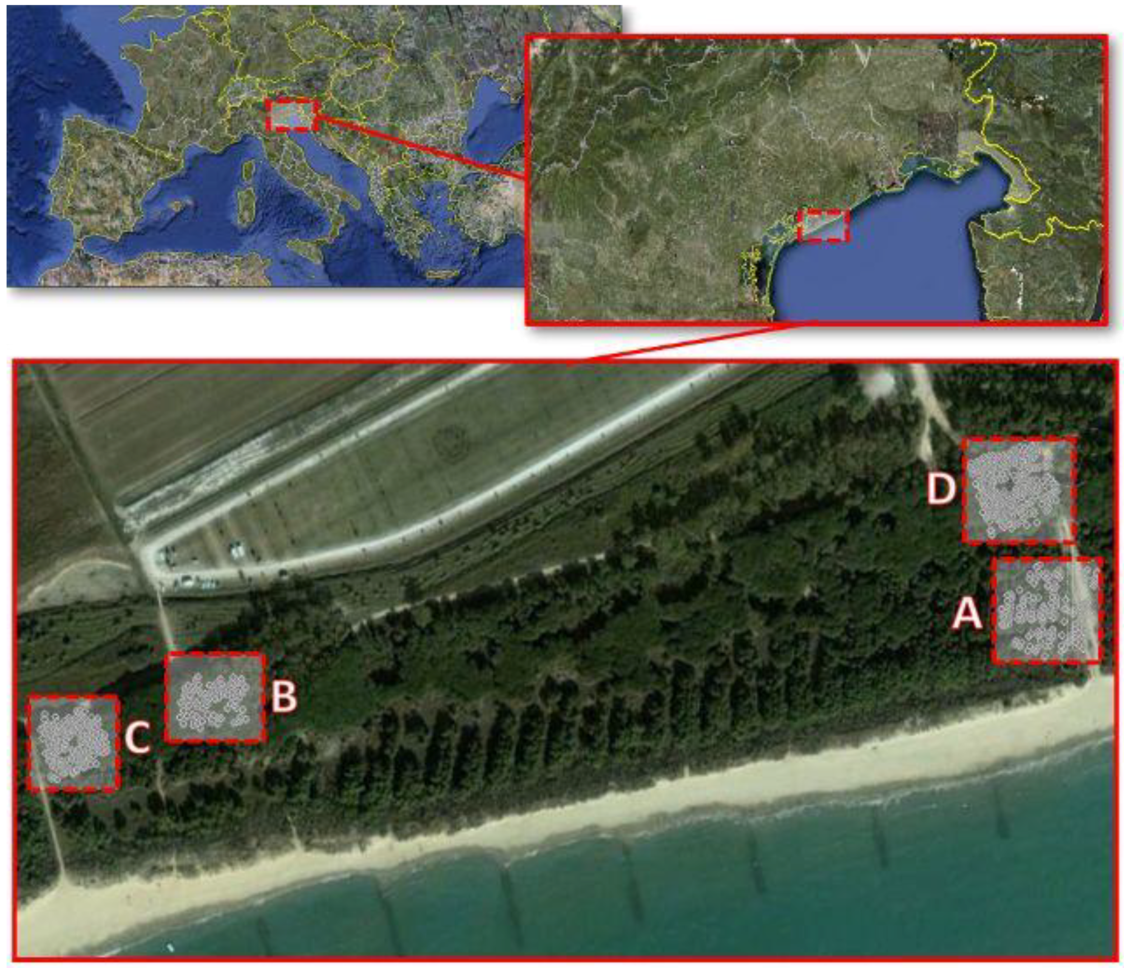
2.1. Study Area and Data Collection

The experimental area is situated in the north-eastern part of Italy, in the Veneto region. Its center is approximately at 12°57′22″ longitude and 45°37′20″ latitude relative to the 1984 World Geodetic System datum (WGS84). It is located in the Mediterranean Basin and falls in the Temperate Oceanic bioclimate. Four areas have been plotted inside an even-aged stand of Pinus pinaster which was introduced by reforestation activity to protect the nearby northbound Pinus pinea stands from marine aerosol. The area borders a shoreline environment towards the south and Pinus pinea stands and grain agriculture fields at the north (Figure 1).

Figure 1. Study area with the four ground-surveyed areas (A-B-C-D).

Figure 1. Study area with the four ground-surveyed areas (A-B-C-D).

The survey campaign was done during the month of November 2008 using a reflector-less Leica TC200 total station to measure stem positions. The plots were georeferenced using a Geotop Hiper Pro GPS receiver to position six tie points in open-sky conditions. The georeference system used is the UTM-WGS84 datum (European Petroleum Survey Group—EPSG code = 32632). This instrument has a dual-frequency receiver which, using RTK connection with a fixed base antenna, allowed precise (±0.01 m) positioning of the six points. At least three of the six tie points were then measured from the total station each time it was positioned in each plot, thus allowing calculation of the position and orientation of the plot itself. Stem coordinates were recorded by measuring angle and distance from the instrument to the stem surface and correcting distance with the stem diameter at breast height, which was also recorded. Heights of all trees whose top was visible along the line-of-sight of the instrument were also recorded. Characteristics of the four areas are listed in Table 1. As can be seen the areas are very similar, except area B which has an empty patch at its south-eastern quadrant and thus has lower tree overall density.

Table 1. Summary of field data: A–D plots, N = number of stems in plot, SD = standard deviation, DBH = breast height diameter.

	Plots
	A	B	C	D
Area, ha	0.1963	0.3847	0.25	0.25
N (N ha−1)	158 (805)	95 (245)	179 (716)	117 (468)
Mean DBH (SD)	0.25 m (0.054)	0.29 m (0.05)	0.28 m (0.064)	0.28 m (0.08)
Mean tree height (SD)	12.06 m (0.89)	12.02 m (1.11)	12.38 m (0.74)	11.95 m (0.76)
Trees with height measured	18	24	21	15

Table 1. Summary of field data: A–D plots, N = number of stems in plot, SD = standard deviation, DBH = breast height diameter.

	Plots
	A	B	C	D
Area, ha	0.1963	0.3847	0.25	0.25
N (N ha−1)	158 (805)	95 (245)	179 (716)	117 (468)
Mean DBH (SD)	0.25 m (0.054)	0.29 m (0.05)	0.28 m (0.064)	0.28 m (0.08)
Mean tree height (SD)	12.06 m (0.89)	12.02 m (1.11)	12.38 m (0.74)	11.95 m (0.76)
Trees with height measured	18	24	21	15

Lidar data was obtained by a sensor mounted on an AS350 B32 helicopter: characteristics of sensor and data are listed in Table 2. Point accuracy provided by the lidar survey company was double‑checked using four of the six control points measured with GPS for plot positioning. All four points had a positional error well within given accuracy range, thus no further corrections were necessary.

Table 2. Lidar flight characteristics. Z refers to vertical accuracy, XY to planar accuracy.

Characteristic	Value
Date	8 April 2008
Average flight height	800 m
Average density	5 pts/m2
Pulse frequency	33 kHz
Sensor model	OPTECH ALTM 3033
Scan angle	±10°
Laser wavelength	1,064 nm
Expected point accuracy (1 sigma)	Z = 0.15 m XY = 0.3

Table 2. Lidar flight characteristics. Z refers to vertical accuracy, XY to planar accuracy.

Characteristic	Value
Date	8 April 2008
Average flight height	800 m
Average density	5 pts/m2
Pulse frequency	33 kHz
Sensor model	OPTECH ALTM 3033
Scan angle	±10°
Laser wavelength	1,064 nm
Expected point accuracy (1 sigma)	Z = 0.15 m XY = 0.3

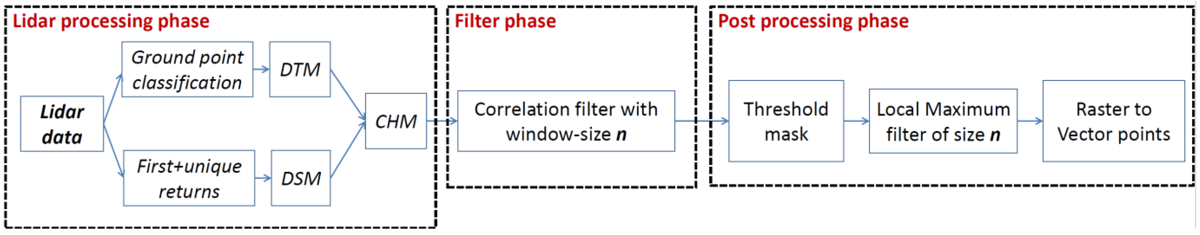
2.2. Lidar Processing and Software Used

Processing consists of several steps which take as input the lidar point cloud and give as output a vector point map with inferred tree-top position and heights. It can be divided into a lidar-processing phase, a filter phase and a post-processing phase (Scheme 1). The lidar processing phase was done using Terrasolids’ TerraScan module for Benteley Microstation. The filter phase and the post‑processing phase are done using GRASS (Geographic Resources Analysis Support System) open source software. GRASS’s open code and raster-processing libraries provided the opportunity to implement the correlation filter used in the filter phase and integrate it in the GRASS environment. The module is available at author’s webpage and can be easily integrated into existing GRASS Linux distributions or compiled for any platform (comments are welcome). The resulting vector points in output from the filter procedure are spatially analyzed using R statistical language [24] procedures.

Scheme 1. Procedure of filter application in its three phases.

Scheme 1. Procedure of filter application in its three phases.

2.2.1. Lidar Processing Phase

In the lidar processing phase the point cloud is classified into ground points and not-ground points using Axelsson’s iterative triangulation algorithm [25]. Successive gridding of the triangulated ground surface into a 0.5 m resolution raster produced the digital terrain model (DTM). The digital surface model (DSM) was created at the same resolution from gridding the triangulated surface of first + unique return points. No other process was necessary because neither buildings nor other disturbances (power lines) for vegetation-detection were present in the area. The difference between the DSM and the DTM provides the canopy height model (CHM).

2.2.2. Filter Phase

The filter phase consists of application of the correlation filter. This consists of a template matrix where each cell is populated with values using a Gaussian normal function:

$$V(m,n)=\frac{\exp (-\frac{m^2 + n^2}{2{\sigma }^2})}{2\pi {\sigma }^2}$$

(1)

where m and n are column and row number of filter window of size m x n where m = n and are both odd values and σ is the standard deviation. The standard deviation can be set according to tree canopy type. For conical shapes, which require a sharper peak, a low standard deviation (1–3) can be used, whereas more elliptical canopies require a higher standard deviation value (7–10). A value of 10 is used for this study case due to the similarity of such kernel with the canopy shape of Pinus pinaster. Geometrical representations of the template matrix with two different standard deviations can be seen in Figure 2.

Figure 2. A 3D plot of the Gaussian kernel used as template here is shown over a graphical representation of generic canopies. (a) σ = 2 over a conical-shape canopy. (b) σ = 10 over a ellipsoidal-shape canopy.

Figure 2. A 3D plot of the Gaussian kernel used as template here is shown over a graphical representation of generic canopies. (a) σ = 2 over a conical-shape canopy. (b) σ = 10 over a ellipsoidal-shape canopy.

The filter works by calculating the 2-d discrete cross-correlation value between the filter kernel and the underlying corresponding CHM matrix and assigning it to the pixel at the center of the moving window:

(2)

where: r is the normalized correlation value at column i* and row j* which is the center—respectively i* = I − (m − 1)/2 and j* = j − (n − 1)/2 and i and j are the ith and jth row and column in the grid—B is the CHM, A is the kernel matrix with m columns and n rows which have to be odd identical values, B* is the part of CHM window overlapping the kernel (see Figure 3). The denominator in the expression is the standard deviation of values in the kernel and in the overlapped CHM and serves to normalize the result such that −1 ≤ r ≤ 1.

The result of this phase is a raster representation of correlation values which corresponds to the degree of similarity between the template kernel and the corresponding grid values of the CHM. Since the CHM resolution is 0.5 m, and the maximum distance between nearest neighbor trees was found to be 5 m, we tested 5 window sizes; 3 × 3, 5 × 5, 7 × 7, 9 × 9 and 11 × 11 thus covering a real-size from 1.5 m to 5.5 m. Figure 4 depicts a representation of CHM and corresponding correlation map as well as a profile showing the typical ellipsoidal canopy shape.

Figure 3. Schematic representation of CHM grid and kernel matrix window for calculation of 2D cross-correlation value between A (kernel) and B* (CHM). See equation 2 and corresponding explanation for details.

Figure 3. Schematic representation of CHM grid and kernel matrix window for calculation of 2D cross-correlation value between A (kernel) and B* (CHM). See equation 2 and corresponding explanation for details.

Figure 4. (a) CHM grid and (b) corresponding correlation map resulting from the application of a 5 × 5 correlation filter with a mask over values below zero. The normalized correlation values have been scaled ×100. (c) Canopy and terrain profile of transect over area.

Figure 4. (a) CHM grid and (b) corresponding correlation map resulting from the application of a 5 × 5 correlation filter with a mask over values below zero. The normalized correlation values have been scaled ×100. (c) Canopy and terrain profile of transect over area.

2.2.3. Post Processing Phase

The correlation map is processed to extract local maximum correlation values. Masking is first applied to the correlation map in order to only keep cells which present significant correlation using a threshold. An objective method to decide the threshold value had to be found, so it was decided to use the lowest value that would reject the null hypothesis, with a 99% confidence that correlation is not significant. This value, (r), was calculated considering sample size equal to the number of cells in the kernel matrix (n) with t-value (t) relative to corresponding degrees of freedom:

$$r=\frac{t}{\sqrt{n-2+t^2}}$$

(3)

The value of t was chosen relative to a 99% confidence that correlation values above r will be significantly different from no correlation (r = 0). This is done to avoid local maxima detecting correlation values which are actually not significant.

The next step in the post-processing phase is to isolate the local maximum of the correlation values around a neighborhood of the same size as the correlation kernel. This filter assesses if the cell at the center of the window has the highest value and accepts it only if true. There is plentiful documentation in the literature on its use directly on CHM [6,22,23]; in this study it is used on the correlation model and not directly on the canopy height model. The advantage should be that a correlation kernel considers overall shape similarity with the local CHM area, while the local maximum approach directly on CHM does not. The isolated pixels, which represent local maximum, are then converted to points to be analyzed as a point pattern in the R statistical analysis software.

3. Results and Discussion

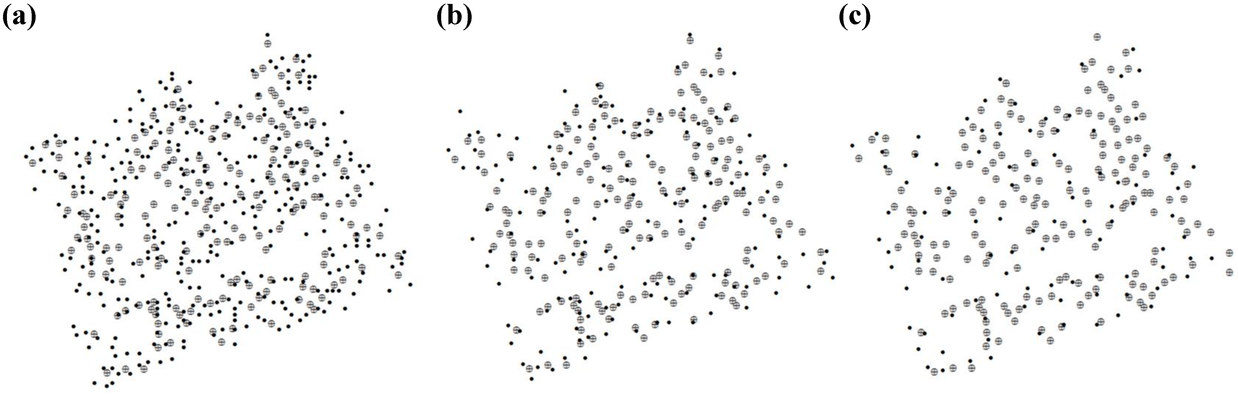
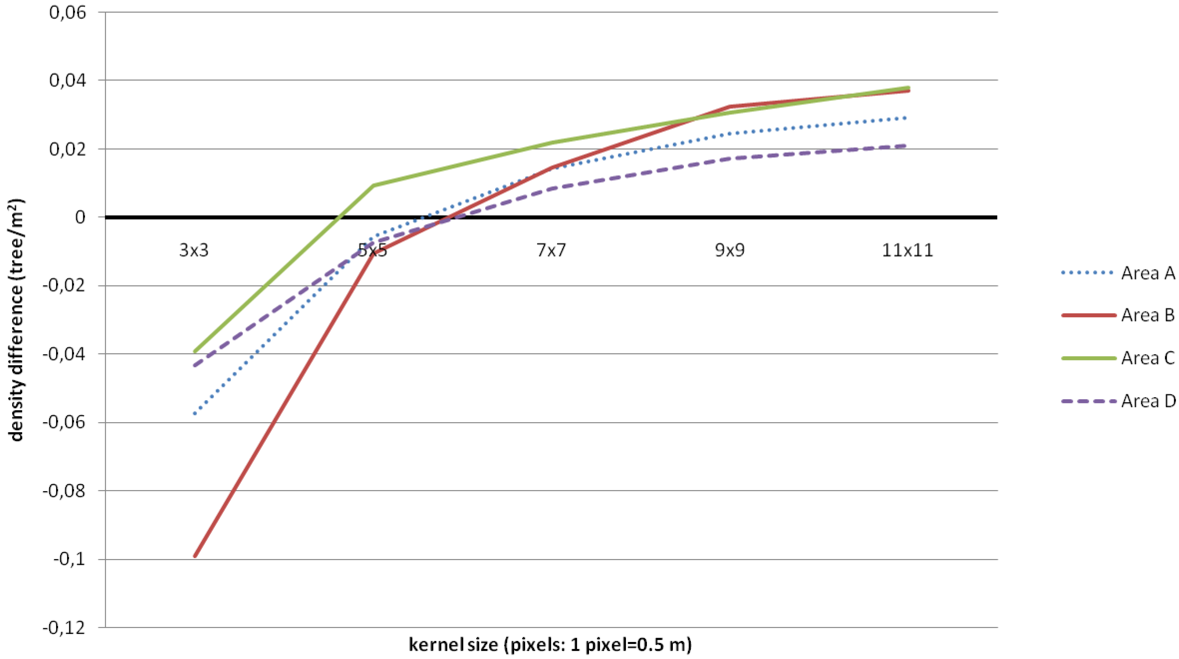
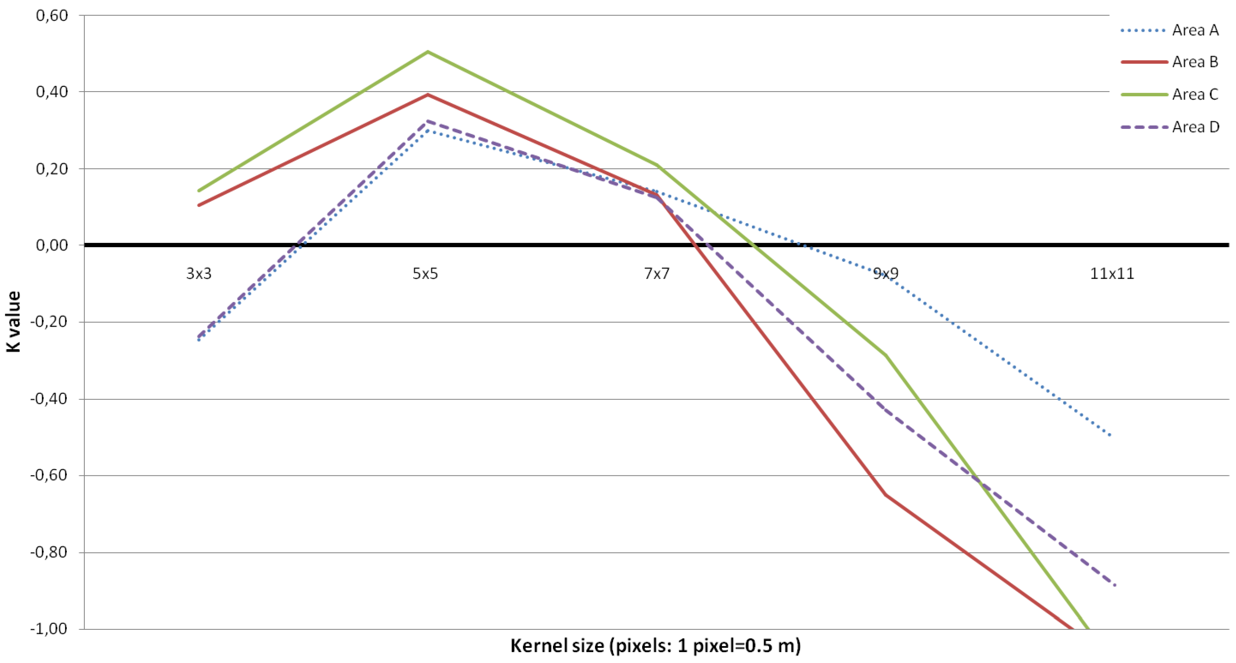
3.1. Tree Density and Position

In Figure 5 the surveyed positions of tree trunks at breast height and of lidar-inferred tree tops from best performing window sizes (3 × 3, 5 × 5 and 7 × 7) are plotted. Tree count and corresponding density are extracted for all tested kernel sizes, and error with ground truth calculated (dD = D_ground-truth − D_{lidar-inferred}) and plotted in Figure 6. From Figure 6, it can be affirmed that the best result of the tree density parameter is obtained using the 5 × 5 kernel. Interpolation of results between window sizes for all areas except area C shows that a theoretical 6 × 6 window would have performed even better. This is most probably influenced by the nearest neighbor distance which shows that the average distance between trees in those three areas is ~2.3 meters. The 5 × 5 window, in our 0.5 meter resolution raster, is the closest size as it embraces a 2.5 × 2.5 area. The fact that it actually under‑estimates the tree count is most probably due to trees whose canopy is completely embedded with another tree, thus making separation very difficult. Area C has a slightly different result, showing a slight over-estimation using the 5 × 5. Since this area has the same characteristics as the others in terms of mean diameter, height and density, the reason might be found in irregular canopy shape. This aspect has to be investigated further as it can provide interesting information on the behavior of the method.

Figure 5. Comparison between surveyed stem position (crossed grey circles) and calculated stem position (smaller filled circles) for area C. (a) 3 × 3 size window, (b) 5 × 5 size window and (c) 7 × 7 size window.

Figure 5. Comparison between surveyed stem position (crossed grey circles) and calculated stem position (smaller filled circles) for area C. (a) 3 × 3 size window, (b) 5 × 5 size window and (c) 7 × 7 size window.

Figure 6. Density error for each kernel size: the difference between surveyed density and lidar–derived density as a function of kernel size.

Figure 6. Density error for each kernel size: the difference between surveyed density and lidar–derived density as a function of kernel size.

An evaluation of accuracy of tree-top position detection was done using an agreement test. Agreement tests improve on simple agreement by considering also the agreement expected by chance and giving an estimated coefficient of agreement. Cohen [28] and Fleiss [29] have proposed different applications for the coefficient of agreement, respectively for categorical items and for categorical ratings in a number of class items. This study case considers reliability of crown-top position correspondence to position of trunk at breast height. These two elements can have a spatial offset, thus the objective is not to estimate absolute position error, but to estimate agreement in tree detection considering expected chance agreement together with omission and commission errors (false negatives and false positives). These last two elements are calculated as complements of the two point sets (ground truth positions and lidar-inferred positions) where matching nearest neighbors between surveyed points and lidar-inferred points are considered as common points in sets:

(4)

where S is the surveyed point set and I is the lidar-inferred point set, C_err is commission errors and O_err is omission errors, M is the matching point set. Matching was done by sorting the results from cross nearest neighbor calculations from smallest to greatest; a point in I is considered as matching a point in S if it is within a threshold distance equal to the average tree distance measured (~2.3 m). Matches have to be unique in the sense that a tree in S cannot match more than one tree in I. Once all trees from ground survey (S) have been matched, eventual remaining points are considered as omission errors, while unmatched points and eventual remaining points from the lidar-inferred (I) set are considered commission errors. Having all this information the kappa coefficient of agreement (K) can be calculated:

$$\begin{array}{l}\mathrm{P}{\mathrm{r}}_a=\frac{N_m}{N_S}\\ C_{err}=\frac{N_c}{N_m+N_c+N_o}\\ O_{err}=\frac{N_o}{N_m+N_c+N_o}\\ \mathrm{P}{\mathrm{r}}_e=C_{err}^2+O_{err}^2\\ K=\frac{\mathrm{P}{\mathrm{r}}_a-\mathrm{P}{\mathrm{r}}_e}{1-\mathrm{P}{\mathrm{r}}_e}\end{array}$$

(5)

where Pr_a is observed agreement and Pr_e is chance agreement, N_m is number of matching points, N_S is number of surveyed points, N_c is number of points assigned as commission errors, and N_o is number of points assigned as omission errors. In Table 3 results are reported and calculated K values are plotted as a function of correlation filter window size in Figure 7. Percentage of tree extraction is the ratio of matched to surveyed tree ratio: N_m/N_S.

The agreement coefficient between tree extraction and measured tree positions shows the best correlation window size to be 5 × 5 for all four areas, in line with the above observations that the scale of the window size has to be proportioned to the scale of the canopy investigated. It is interesting to note that the percentage of tree extractions in Table 3 is always higher for smaller kernel sizes. This of course does not account for false positives and false negatives like the agreement coefficient does and is therefore, misleading. In this context, it can be affirmed that an a priori knowledge of average tree nearest neighbor distance can be used to decide kernel size. This is of course valid for stands which present a spatial distribution which is not clustered, but would work well for regularly spaced trees such as in plantations. For example, poplar plantations are common in this area and in many regions of Italy and are encouraged with incentives given by afforestation programs as well [30]. They could be ideal stands for the application of this method.

Table 3. Coefficient of agreement (K) and percentage of tree extraction (%) for the four areas. KS = kernel size, N_S = total number of ground-truth surveyed tree positions, N_I = total number of lidar-inferred tree tops, N_C = commission error (false positives), N_O = omission error (false negatives) and N_m = number of matching (correct) points.

	Area A (NS = 158)						Area B (NS = 95)
KS	NI	NC	NO	Nm	K	%	NI	NC	NO	Nm	K	%
3 × 3	396	278	40	118	−0.25	74	212	125	8	87	0.11	84
5 × 5	189	86	55	103	0.30	65	91	31	75	60	0.39	68
7 × 7	115	45	88	70	0.14	44	54	14	55	40	0.13	45
9 × 9	74	20	104	54	−0.08	34	28	6	73	22	−0.65	30
11 × 11	53	14	119	39	−0.50	24	22	4	77	18	−1.08	19
	Area C (NS = 179)						Area D (NS = 117)
KS	NI	NC	NO	Nm	K	%	NI	NC	NO	Nm	K	%
3 × 3	359	207	27	152	0.14	91	312	216	21	96	−0.24	82
5 × 5	163	41	57	122	0.50	63	151	69	35	82	0.32	70
7 × 7	98	17	98	81	0.21	42	78	28	67	50	0.13	42
9 × 9	60	5	124	55	−0.29	23	48	20	89	28	−0.43	23
11 × 11	40	5	144	35	−1.09	18	34	13	96	21	−0.89	17

Table 3. Coefficient of agreement (K) and percentage of tree extraction (%) for the four areas. KS = kernel size, N_S = total number of ground-truth surveyed tree positions, N_I = total number of lidar-inferred tree tops, N_C = commission error (false positives), N_O = omission error (false negatives) and N_m = number of matching (correct) points.

	Area A (NS = 158)						Area B (NS = 95)
KS	NI	NC	NO	Nm	K	%	NI	NC	NO	Nm	K	%
3 × 3	396	278	40	118	−0.25	74	212	125	8	87	0.11	84
5 × 5	189	86	55	103	0.30	65	91	31	75	60	0.39	68
7 × 7	115	45	88	70	0.14	44	54	14	55	40	0.13	45
9 × 9	74	20	104	54	−0.08	34	28	6	73	22	−0.65	30
11 × 11	53	14	119	39	−0.50	24	22	4	77	18	−1.08	19
	Area C (NS = 179)						Area D (NS = 117)
KS	NI	NC	NO	Nm	K	%	NI	NC	NO	Nm	K	%
3 × 3	359	207	27	152	0.14	91	312	216	21	96	−0.24	82
5 × 5	163	41	57	122	0.50	63	151	69	35	82	0.32	70
7 × 7	98	17	98	81	0.21	42	78	28	67	50	0.13	42
9 × 9	60	5	124	55	−0.29	23	48	20	89	28	−0.43	23
11 × 11	40	5	144	35	−1.09	18	34	13	96	21	−0.89	17

Figure 7. Kappa coefficient of agreement of tree detection for each kernel size.

Figure 7. Kappa coefficient of agreement of tree detection for each kernel size.

3.2. Tree Height Distribution

As reported in Table 1, a sub-selection of trees in each plot were measured for height. The measured height distribution is compared with the height extracted after tree extraction. This is done by querying the CHM pixel value underneath the lidar-inferred tree-top position using results from the 5 × 5 kernel size which proved to have the highest accuracy. Measured tree height and corresponding lidar-inferred height are used to calculate error by subtracting measured value from inferred value. Error distribution statistics are reported in Table 4.

Table 4. Error statistics for height measures: N = Number of trees with height measurements, SD = standard deviation, M_M = Mean of measures, M_L = mean of lidar inferred heights, ME = mean of errors, MAE = mean of absolute errors, RMSE = root of the mean of sum over squared errors, % = RMSE relative to mean measured height.

	PLOTS
	A	B	C	D
N	18	24	21	15
MM (SD)	12.06 m (0.89)	12.02 m (1.11)	12.38 m (0.74)	11.95 m (0.76)
ML (SD)	11.94 m (0.47)	11.95 m (0.67)	12.26 m (0.54)	11.54 m (0.79)
ME	−0.12	−0.063	−0.123	−0.41
MAE	0.54	0.504	0.422	0.70
RMSE	0.624	0.622	0.528	1.01
%	5.23	5.21	4.31	8.76

Table 4. Error statistics for height measures: N = Number of trees with height measurements, SD = standard deviation, M_M = Mean of measures, M_L = mean of lidar inferred heights, ME = mean of errors, MAE = mean of absolute errors, RMSE = root of the mean of sum over squared errors, % = RMSE relative to mean measured height.

	PLOTS
	A	B	C	D
N	18	24	21	15
MM (SD)	12.06 m (0.89)	12.02 m (1.11)	12.38 m (0.74)	11.95 m (0.76)
ML (SD)	11.94 m (0.47)	11.95 m (0.67)	12.26 m (0.54)	11.54 m (0.79)
ME	−0.12	−0.063	−0.123	−0.41
MAE	0.54	0.504	0.422	0.70
RMSE	0.624	0.622	0.528	1.01
%	5.23	5.21	4.31	8.76

It can be seen that lidar inferred height is underestimated in all four plots, probably due to the point density which is not very high (4–5 points per square meter) as has already been reported in the literature [16,31,32,33,34]. The mean absolute error is lower than other tests in different contexts [33,34] because some factors which influence height estimation are in this case ideal; terrain is flat and canopies are in a single layer. Another point worth mentioning is that the canopy shape is such that the slope value around the tree top is very low. For this reason a small positional error does not imply a significant height error like it would in the case of conical canopies.

4. Conclusions

This paper discussed results of a different approach towards tree extraction, positioning, and height estimation, on a single tree basis. Forest environments are, in reality, varied, and this method does not pretend to be accurate in all contexts, but wants to give an alternative to other methods which might work less well in situations like the one presented in the test site. As mentioned in the discussion section, the ideal context for this application should be regular spaced trees, without a significant dominated layer and an ellipsoidal shaped canopy. Conical shaped canopies will benefit mostly from a local maximum filter approach as application of a correlation filter would be redundant. A clustered spatial distribution would imply embedded canopies which are harder to detect (with any approach). The kernel size in relation to the canopy size is an important parameter as a larger window would embrace multiple canopies thus giving low correlations also when centered on a tree top, whereas smaller windows would be subject to “noise” effects of canopy morphology resembling tree tops and thus overestimate the number of tree positions. It would be interesting to conduct future investigations to understand the effect of lidar point density and respective CHM resolution on the filter performance. It is likely that higher point densities and higher CHM resolutions improve results because the matching process would be more precise. This method could be applied to stands with the preferred characteristic of having few or no dominant trees and where canopy shape makes it difficult for other methods to give good results. The ability to obtain stand density and spatial distribution of its elements over large areas using a semi-automatic process can be of great help as input to inventories and as parameters for derived ecological indices. Also less ground-truth surveys would be needed and could just be used to control the results, bringing an economical advantage.

References

1. Wiensa, J.; Sutter, R.; Anderson, M.; Blanchard, J.; Barnett, A.; Aguilar-Amuchasteguib, N.; Averyd, C.; Lained, S. Selecting and conserving lands for biodiversity: the role of remote sensing. Remote Sens. Environ. 2009, 113, 1370–1381. [Google Scholar] [CrossRef]
2. Scanlan, I.; McElhinny, C.; Turner, P. A methodology for modelling Canopy structure: An exploratory analysis in the tall Wet Eucalypt forests of Southern Tasmania. Forests 2010, 1, 4–24. [Google Scholar] [CrossRef]
3. Dubayah, R.; Blair, J. Lidar remote sensing for forestry applications. J. For. 2000, 98, 44–46. [Google Scholar]
4. Falkowski, M.J.; Evans, J.S.; Martinuzzi, S.; Gessler, P.E.; Hudak, A.T. Characterizing forest succession with lidar data: An evaluation for the Inland Northwest, USA. Remote Sens. Environ. 2009, 113, 946–956. [Google Scholar]
5. Tesfamichael, S.G.; Ahmed, F.; van Aardt, J.A.N.; Blakeway, F. A semi-variogram approach for estimating stems per hectare in Eucalyptus grandis plantations using discrete-return lidar height data. For. Ecol. Manage. 2009, 258, 1188–1199. [Google Scholar] [CrossRef]
6. Korpela, I.; Dahlin, B.; Schäfer, H.; Bruun, E.; Haapaniemi, F.; Honkasalo, J.; Ilvesniemi, S.; Kuutti, V.; Linkosalmi, M.; Mustonen, J.; Salo, M.; Suomi, O.; Virtanen, H. Single-tree forest inventory using lidar and aerial images for 3d treetop positioning, species recognition, height and crown width estimation. Int. Arch. Photogram. Remote Sens. Spat. Inf. Sci. 2007, 36-3/W52, 227–234. [Google Scholar]
7. Hyyppä, J.; Inkinen, M. Detecting and estimating attributes for single trees using laser scanner. Photogramm. J. Finl. 1999, 16, 27–42. [Google Scholar]
8. Suarez, J.C.; Ontiveros, C.; Smith, S.; Snape, S. Use of airborne LiDAR and aerial photography in the estimation of individual tree heights in forestry. Comput. Geosci. 2005, 31, 253–262. [Google Scholar] [CrossRef]
9. Popescu, S.C.; Wynne, R.H.; Nelson, R.F. Estimating plot-level tree heights with lidar: local filtering with a canopy-height based variable window size. Comput. Electron. Agric. 2002, 37, 71–95. [Google Scholar] [CrossRef]
10. Popescu, S.C.; Wynne, R.H. Seeing the trees in the forest: using lidar and multispectral data fusion with local filtering and variable window size for estimating tree height. Photogram. Eng. Remote Sens. 2004, 70, 589–604. [Google Scholar] [CrossRef]
11. Barilotti, A.; Sepic, F.; Abramo, E.; Crosilla, F. Improving the morphological analysis for tree extraction: a dynamic approach to lidar data. Int. Arch. Photogram. Remote Sens. Spat. Inf. Sci. 2007, 36-3/W52, 26–31. [Google Scholar]
12. Popescu, S.C.; Wynne, R.H.; Scrivani, J.A. Fusion of small-footprint lidar and multispectral Data to estimate plot-level volume and biomass in deciduous and pine forests in virginia, USA. For. Sci. 2004, 50, 551–565. [Google Scholar]
13. Hill, R.A.; Thomson, A.G. Mapping woodland species composition and structure using airborne spectral and LiDAR data. Int. J. Remote Sens. 2005, 26, 3763–3779. [Google Scholar] [CrossRef]
14. Huang, H.; Gong, P.; Cheng, X.; Clinton, N.; Li, Z. Improving measurement of forest structural parameters by co-registering of high resolution aerial imagery and low density LiDAR data. Sensors 2009, 9, 1541–1558. [Google Scholar] [CrossRef] [PubMed]
15. Hyde, P.; Dubayah, R.; Peterson, B.; Blair, J.B.; Hofton, M.; Hunsaker, C.; Knox, R.; Walker, W. Mapping forest structure for wildlife habitat analysis using waveform lidar: Validation of montane ecosystems. Remote Sens. Environ. 2005, 96, 427–437. [Google Scholar] [CrossRef]
16. Magnussen, S.; Boudewyn, P. Derivations of stand heights from airborne laser scanner data with canopy-based quantile estimators. Can. J. For. Res. 1998, 28, 1016–1031. [Google Scholar] [CrossRef]
17. Næsset , E. Accuracy of forest inventory using airborne laser scanning: evaluating the first Nordic full-scale operational project. Scan. J. For. Res. 2004, 19, 554–557. [Google Scholar]
18. Barilotti, A.; Sepic, F.; Abramo, E. Automatic detection of dominated vegetation under canopy using Airborne Laser Scanning data. In Proceedings of the Silvilaser 2008: 8th International Conference on LiDAR Applications in Forest Assessment and Inventory; Edinburgh, UK, September 2008, Hill, R., Rossette, J., Suárez, J., Eds.; Bournemouth University: Edinburgh, UK, 2008; pp. 134–143. [Google Scholar]
19. Maltamo, M.; Packalén, P.; Yu, X.; Eerikäinen, K.; Hyyppä, J.; Pitkänen, J. Identifying and quantifying structural characteristics of heterogeneous boreal forests using laser scanner data. For. Ecol. Manage. 2005, 216, 41–50. [Google Scholar] [CrossRef]
20. Potetz, B.; Lee, T.S. Statistical correlations between two-dimensional images and three-dimensional structures in natural scenes. J. Opt. Soc. Am. A 2003, 20, 1292–1303. [Google Scholar] [CrossRef]
21. Grudin, M.A. On internal representations in face recognition systems. Pattern Recognit. 2000, 33, 1161–1177. [Google Scholar] [CrossRef]
22. Barilotti, A.; Sepic, F.; Abramo, E.; Crosilla, F. Improving the morphological analysis for tree extraction: a dynamic approach to lidar data. Int. Arch. Photogram. Remote Sens. Spat. Inf. Sci. 2007, 36-3/W52, 26–31. [Google Scholar]
23. Blundell, B.S. Local gradient and local maximum analysis of lidar data for tree crown identification. In Proceedings of ASPRS 2008 Annual Conference, Portland, OR, USA, 28 April–2 May 2008.
24. R Development Core Team. R: A Language and Environment for Statistical Computing; R Foundation for Statistical Computing: Vienna, Austria, 2007. [Google Scholar]
25. Axelsson, P.E. Processing of laser scanner data—algorithms and applications. ISPRS J. Photogram. Remote Sens. 1999, 54, 138–147. [Google Scholar] [CrossRef]
26. Matsugami, H.; Shimizu, Y.; Omasa, K. Detection of tree apexes from helicopter-borne scanning lidar data using local maximum filtering. Phyton 2005, 45, 501–505. [Google Scholar]
27. Morsdorf, F.; Meiera, E.; Itten, K.I.; Dobbertin, M.; Allgower, B. LIDAR-based geometric reconstruction of boreal type forest stands at single tree level for forest and wildland fire management. Remote Sens. Environ. 2004, 92, 353–362. [Google Scholar]
28. Cohen, J. A coefficient of agreement for nominal scales. Educ. Psychol. Meas. 1960, 20, 37–46. [Google Scholar]
29. Fleiss, J.L. Statistical Methods for Rates and Proportions; John Wiley: New York, NY, USA, 1981; pp. 38–46. [Google Scholar]
30. Tassone, V.C.; Wesseler, J.; Nescib, F.S. Diverging incentives for afforestation from carbon sequestration: an economic analysis of the EU afforestation program in the south of Italy. For. Policy Econ. 2004, 6, 567–578. [Google Scholar] [CrossRef]
31. Nilsson, M. Estimation of tree heights and stand volume using an airborne lidar system. Remote Sens. Environ. 1996, 56, 1–7. [Google Scholar] [CrossRef]
32. Clark, M.L.; Clark, D.B.; Roberts, D.A. Small-footprint lidar estimation of sub-canopy elevation and tree height in a tropical rain forest landscape. Remote Sens. Environ. 2004, 91, 68–89. [Google Scholar] [CrossRef]
33. Brandtberg, T.; Warner, T.A.; Landenberger, R.E.; McGraw, J.B. Detection and analysis of individual leaf-off tree crowns in small footprint, high sampling density lidar data from the eastern deciduous forest in North America. Remote Sens. Environ. 2003, 85, 290–303. [Google Scholar] [CrossRef]
34. Gaveau, D.L.A.; Hill, R.A. Quantifying canopy height underestimation by laser pulse penetration in small-footprint airborne laser scanning data. Can. J. Remote Sens. 2003, 29, 650–657. [Google Scholar] [CrossRef]