1. Introduction
In May 1999 the SMOS Earth Explorer Opportunity mission [
1,
2] was selected by ESA to provide global soil moisture and sea salinity maps which are key variables in weather, climate and extreme event forecasts. As a secondary objective, data acquired over ice/snow regions may be used to indicate climate changes due to the greenhouse effect. SMOS’ single payload is MIRAS, an innovative 2-D L-band aperture synthesis interferometric radiometer that will be able to measure the full modified Stokes emission vector from a wide 2-D field of view (swath ~800 km, incidence angles from 0° to ~60°). An important feature of this instrument is that, as the satellite moves along its track, a collection of brightness temperatures emitted from the same area on the Earth will be observed under a large range of incidence angles. As a result, the variation of the emissivity as a function of the incidence angle can be exploited in the retrieval of soil moisture and vegetation parameters. This new capability predicts better results than those obtained with other existing radiometers that scan the surface at a single incidence angle. However, as in any inversion problem in geophysical sciences and engineering, the retrieval of soil moisture relies on the accuracy of both the forward emission models (vegetation description and numerical emission model) used to develop the inversion procedure over the range of observed incidence angles, and on the quality of the auxiliary data [
3]. To improve these models, a number of field experiments have been conducted both over land and over sea [
4]. In the case we are dealing with, the vegetation and soil layers must be modeled together to develop an accurate forward model. Models reported in the literature provide the first two modified Stokes emission elements (
Tv,
Th) as a function of frequency and biophysical parameters of soil and vegetation, but not -to our knowledge- the third and fourth modified Stokes elements (
TU and
TV).
In this work a numerical model is presented to efficiently compute the complete modified Stokes emission vector (
Tv,
Th,
TU and
TV) of vegetation-covered soils at low microwave frequencies over a wide range of incidence angles, as required for future retrieval algorithms suitable to the SMOS mission. Simulations have been compared to SMOS REFLEX 2003 radiometric data and to the retrieved vegetation opacity and albedo estimated using the
τ-ω model as forward model in the minimization algorithm [
5]. This comparison gives a clue on the confidence of both models (the complete electromagnetic model and the simplified
τ-ω model) to describe the emissivity of vegetation-covered soils and helps pointing out their weaknesses.
The text is organized as follows.
Section 2 reviews the basic concepts on emission theory.
Section 3 and
Section 4 describe the possibilities for modeling the scenario of a vegetation-covered soil from the geometric and electromagnetic points of view, respectively. Finally,
Section 5 presents the inter-comparison of simulation results modeling the scenario of the SMOS REFLEX 2003 field experiment and the experimental data, including the variation of the emissivity, single-scattering albedo and extinction with the incidence angle.
5. Comparison with Experimental Data from a Vineyard: SMOS REFLEX 2003 Field Experiment
The SMOS REFerence pixel L-band EXperiment (SMOS REFLEX) 2003 took place at the València Anchor Station (VAS, 39°33' N, 1°17' W), València, Spain, from day of year (DoY) 181 to 191, 2003. During the experiment period, the weather was very dry and warm, and in order to get a wide range of soil moisture values, the field was irrigated twice on DoY 182 and 185, and left to dry out. Concurrently with the radiometric measurements, the gravimetric soil moisture, the temperature and the roughness were measured, and the vines were fully characterized (water content, grapevine size, branch distributions, etc.) [
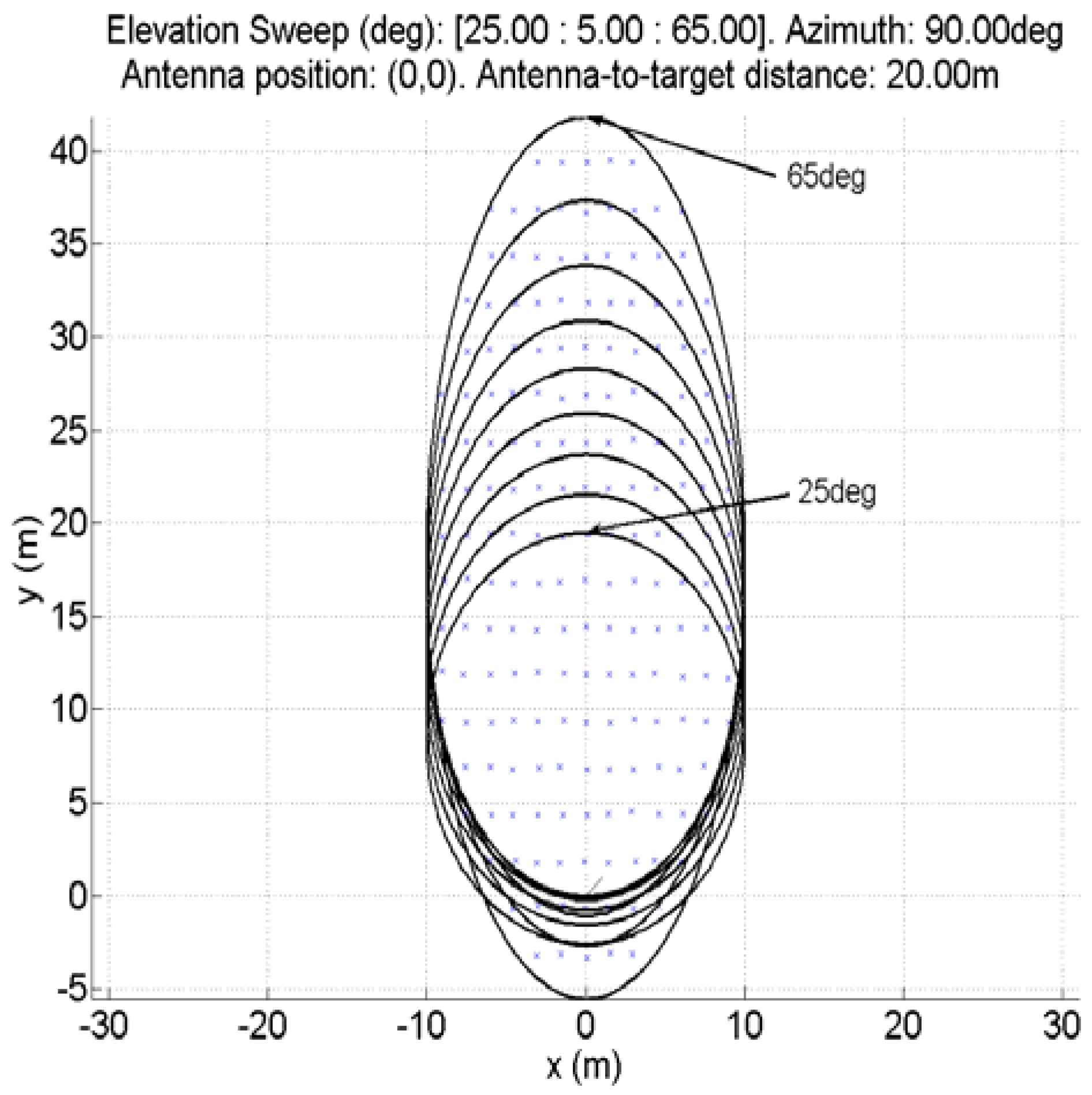
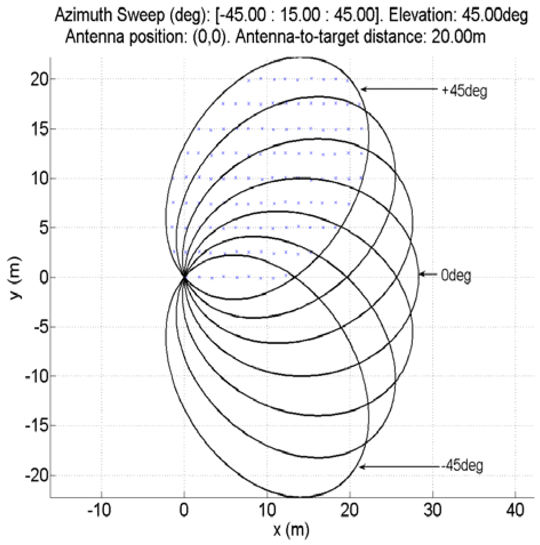
5]. Radiometric measurements were acquired at incidence angles from 25° to 65° (
Figure 7), and at azimuth angles from 45° to 135° with respect to the
X-axis (or ± 45° with respect to the
Y-axis,
Figure 8). The antenna-to-target distance is defined as the distance between the sensor and the central point of the ellipse formed by the projected field-of-view over the soil. This distance was kept constant for both sweeps: elevation and azimuth.
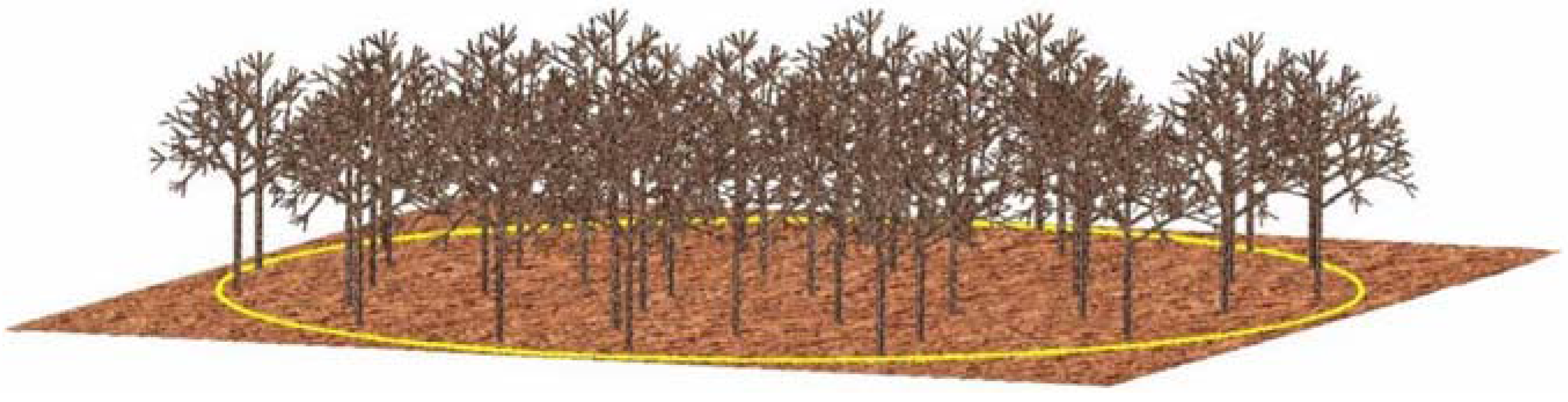
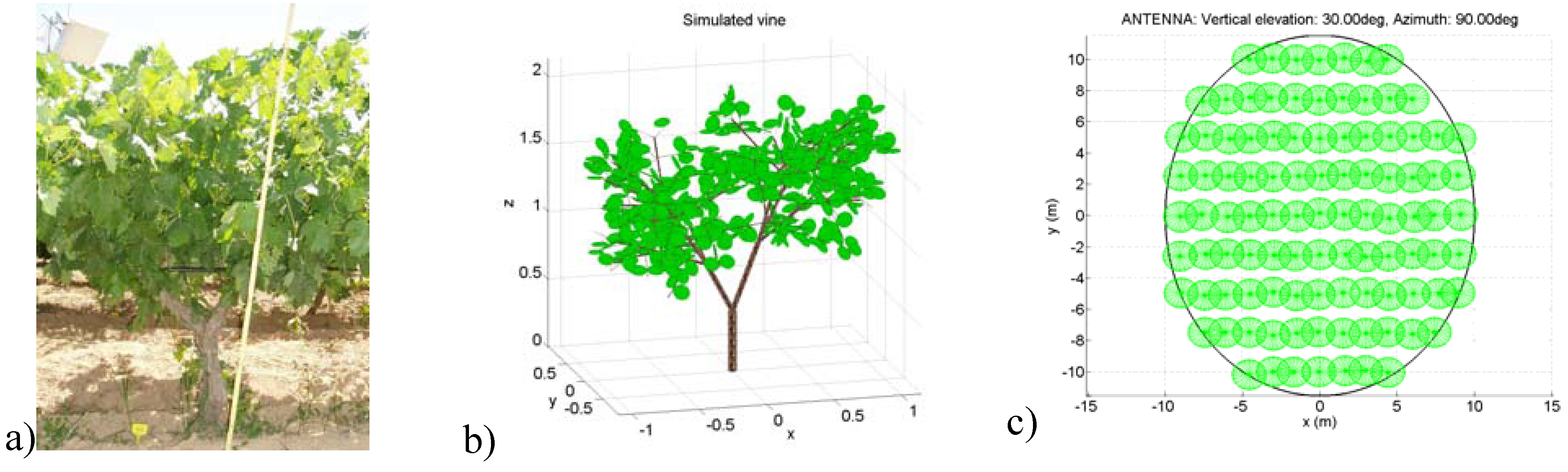
The vines in this field are taller than others in the Mediterranean region, showing an average height of 1.63 m and width of 1.45 m (
Figure 5a), and are planted on a 1.5 m × 2.5 m grid (
Figure 5c; Table I of [
5]). During the experiment, the measured volumetric water content was approximately 9-10 kg/m
2, from which 39.2% corresponded to the grapes, 31.5% to the stem, 10.5% to the primary branches, 2.5% to the secondary branches, 2.5% to the tertiary branches, and the rest to the leaves. The measured leaf area index (
LAI) ranged from about 0.9 m
2/m
2 to 3.4 m
2/m
2.
Figure 7.
Field-Of-View of the antenna footprints for incidence angles from 25° to 65° in 5° steps (azimuthal angle equal to 90°).
Figure 7.
Field-Of-View of the antenna footprints for incidence angles from 25° to 65° in 5° steps (azimuthal angle equal to 90°).
Figure 8.
Field-Of-View of the antenna footprints for azimuthal angles from -45° to +45° in 15° steps (incidence angle equal to 45°).
Figure 8.
Field-Of-View of the antenna footprints for azimuthal angles from -45° to +45° in 15° steps (incidence angle equal to 45°).
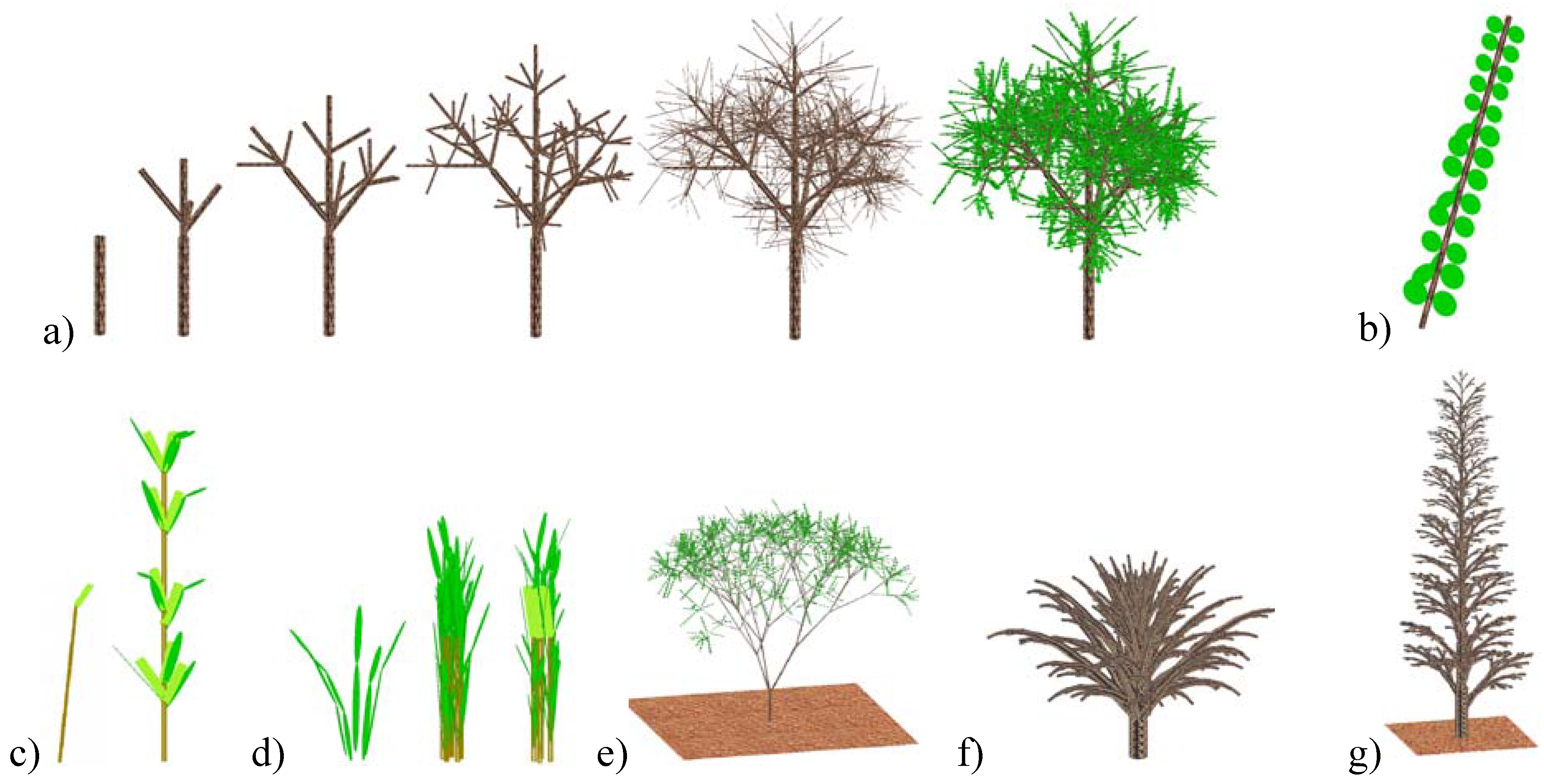
The plant has been modeled with 27 discrete branches and 195 stems, accounting for a volume of 5.58 and 0.79 dm
3, respectively, and a total surface area of 1.58 m
2 (
Figure 5b). The number of leaves equivalent to an approximate
LAI of 1.57 m
2/m
2 is 557, and they were modeled as flattened ellipsoids with semi-axes 6 cm and 5.5 cm, and 1 mm thickness. The volume occupied by the leaves is 5.77 dm
3, whereas the surface is 11.75 m
2. The grapes presented an average radius of ~1.1 cm, and the dry matter fraction was ~ 30%. The total number of grapes (791) is computed so that the volume water content (
VWC) of the grapes corresponds to the measured one (39.2 % of the total
VWC = 4.41 dm
3).
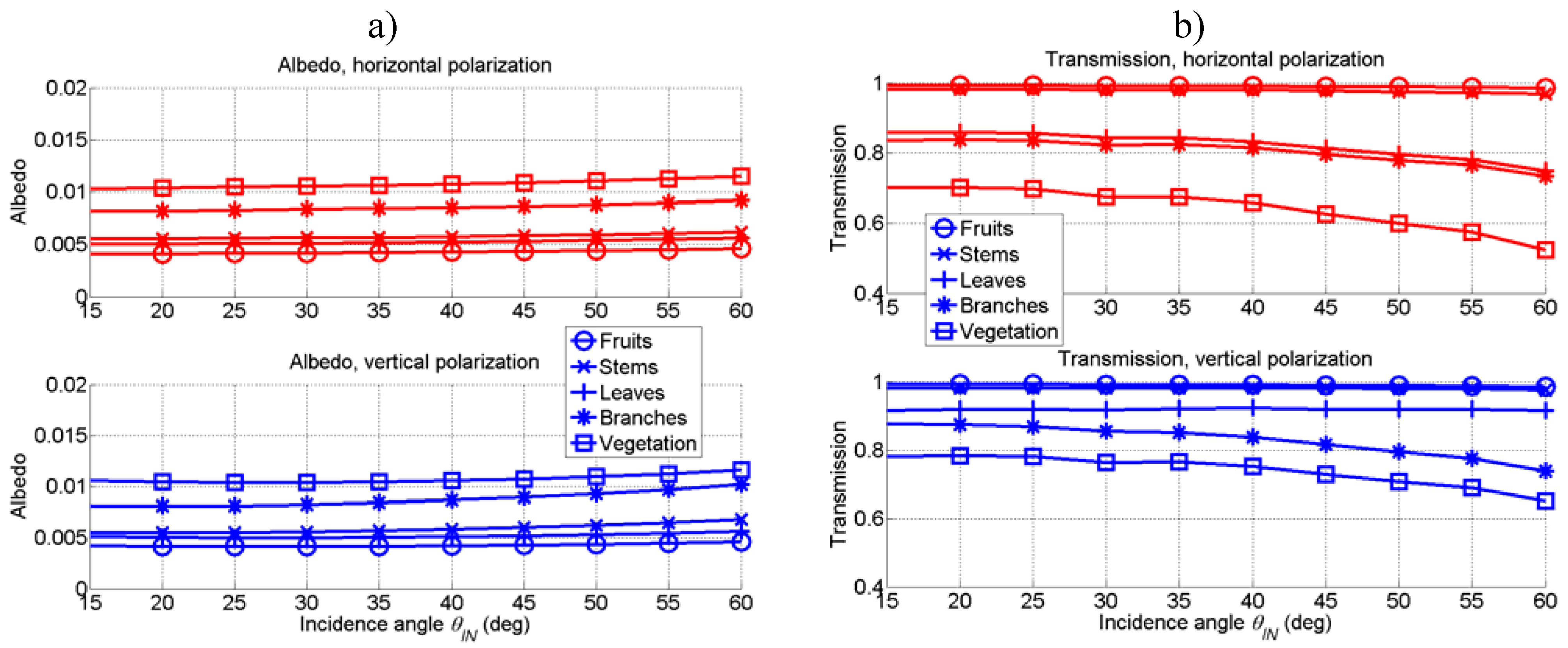
Figure 9.
a) Computed albedo for the different components of the vegetation layer (fruits, stems, leaves and branches) and total single-scattering albedo (vegetation). b) Computed transmissivity for the different components of the vegetation layer (Fruits, Stems, Leaves and Branches) and total transmissivity coefficient (Vegetation).
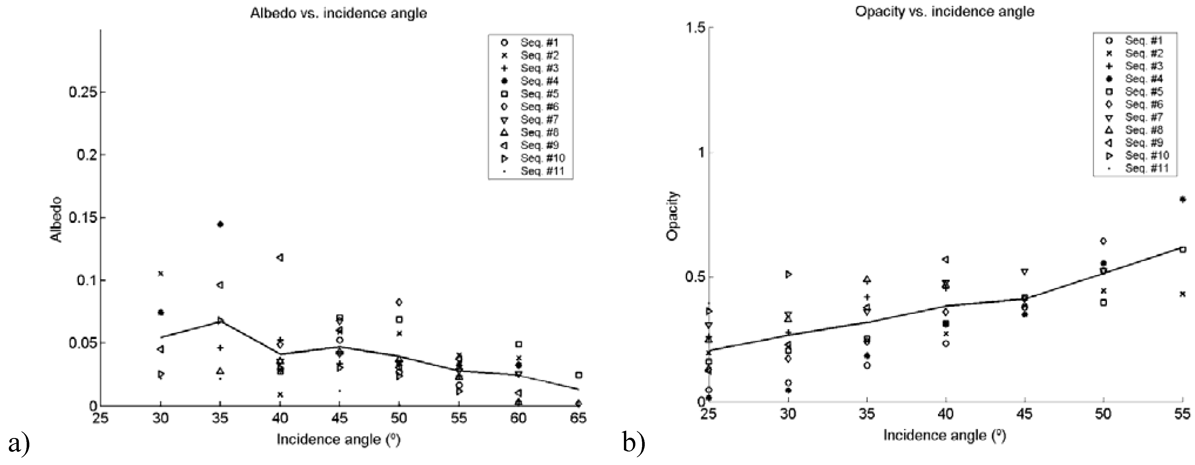
Figure 9a presents the computed single-scattering albedo of the vegetation layer and the individual contributions of the different components of the vegetation (fruits, stems, leaves and branches). The predicted albedo is very similar at both polarizations, it is mostly contributed by the branches, and it matches quite well the one obtained by fitting the radiometric measurements to the
τ-ω model [Equation (1)], specially at high incidence angles (
Figure 10a from [
5]). However, the fitted albedo slightly decreases at higher incidence angle, whereas the simulated one is nearly constant or shows a minimal increase.
Figure 9b presents the total transmissivity of the vegetation as well as the contributions to the total transmissivity (ϒ = e
-τ) of the different components of the vegetation layer separately in horizontal and vertical polarization. At vertical polarization. the predicted value at nadir agrees very well with the opacity (
τ) fitted by adjusting the radiometric measurements to the
τ-ω model (
Figure 10b from [
5]): at
θ = 0°,
τ = 0.21 and ϒ = e
-τ = 0.81, and at
θ = 55°,
τ = 0.61 and ϒ = e
-τ = 0.54. At high incidence angles (~ 55°) the model seems to underestimate it, specially at vertical polarization where the predicted transmissivity is higher than the fitted one. However, it has to be recalled that, as pointed out in [
5], the matching of the radiometric data to the
τ-ω model usually employed at L-band was only possible for incidence angles smaller than 50°, in some cases at 55°, and never above 60°. Therefore, the inter-comparison of the predicted values has to be restricted to incidence angles smaller than 50°. As expected from the orientation and shape of the different vegetation parts,
Figure 9b confirms that the main contribution to the extinction coefficient comes from both branches and leaves at horizontal polarization, and mainly from the branches at vertical polarization.
Figure 10.
a) Albedo vs incidence angle. b) Opacity in Nepers vs incidence angle. Dots represent the retrieved value for each sequence and all azimuth angles, and line plots the mean value (
Figure 8 from [
5]).
Figure 10.
a) Albedo vs incidence angle. b) Opacity in Nepers vs incidence angle. Dots represent the retrieved value for each sequence and all azimuth angles, and line plots the mean value (
Figure 8 from [
5]).
Numerical experiments varying the size and
VWC of the grapes predict only a variation of the single-scattering albedo with the scatterers’ size, whereas the vegetation attenuation is nearly independent of the
VWC. This confirms that in general the attenuation is dominated by the water content in the branches (and in the leaves at horizontal polarization), while grapes (and leaves at vertical polarization) exhibit mostly a scattering behavior [
21].
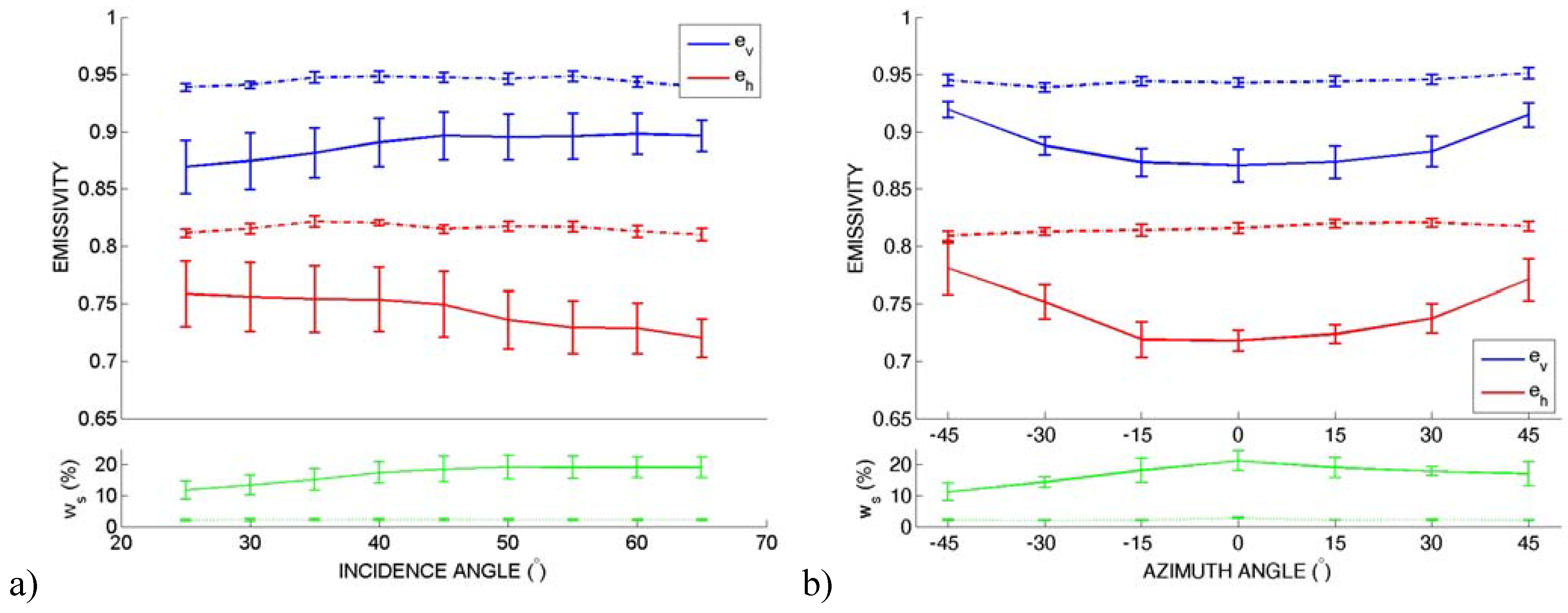
Figure 11a shows the measured emissivities at horizontal and vertical polarizations for a wet (solid line) and a dry day (dashed line). Lines represent the mean value at each incidence angle for the scans at different azimuth angles (from -45° to 45°), and bars represent the associated geophysical fluctuations (rms values). Note that the fluctuations in DoY 185 (wet soil, solid line) are much higher than in DoY 181 (dry soil, dashed-dotted line), due to the variability of the soil moisture in the field, which was due to the gentle slopes and the presence of the vegetation (soil was wetter below the plants, and drier between them).
Figure 11b shows the mean value (solid and dashed-dotted lines) and rms values (bars) of the emissivity as a function of the azimuth angle, averaged for all incidence angles for two representative days of experiment (wet day: DoY 185 solid line, and dry day: DoY 181, dash-dotted line). As it can be appreciated, the soil moisture content was slightly higher around azimuth ~0°, due to the gentle slopes of the terrain, which translates into a marked azimuthal signature, not attributable (at least to first order) to an azimuthal signature associated to the vegetation or the planting pattern. Again, in dry conditions, the azimuthal signature is negligible.
Figure 11.
Emissivity at vertical and horizontal polarizations as a function of the incidence and azimuth angles. a) Mean value and standard deviation of the emissivity and of the ground-truth soil moisture as a function of the incidence angle and for all azimuth angles. DoY 185 (solid line) and DoY 181 (dashed-dotted line) have been represented. Blue and red indicate vertical and horizontal polarizations, respectively. b) Mean value and standard deviation of the emissivity as a function of the azimuth angle, for all incidence angles. Blue and red indicate vertical and horizontal polarizations, respectively. Values for two representative days of experiment have been represented: DoY 185 (solid line), and 181 (dash-dotted line). The averaged soil moisture at each observation position has been included (green lines).
The soil moisture variability complicates the intercomparison with numerical model predictions. Therefore, average values over the field have been taken, at the expense of larger error bars.
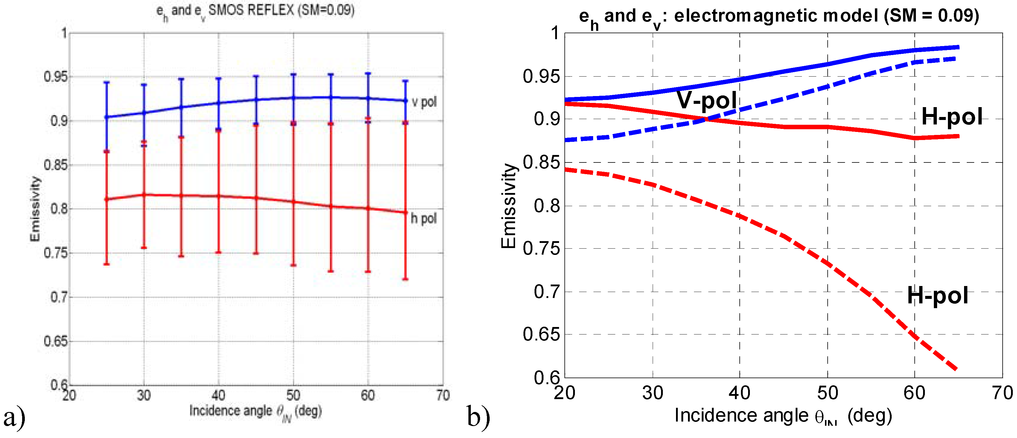
Figure 12a shows the measured emissivities at horizontal and vertical polarizations for an average soil moisture of approximately 9%. Lines represent the mean value at each incidence angle for the scans at different azimuth angles (from -45° to 45°), and bars represent the associated geophysical fluctuations (rms values).
Figure 12b shows the bare soil emission computed using the τ- ω model (
Section 2.1, dash-dot line) and the RTE for soil and vines (
Section 2.2, solid line). As it can be appreciated, the agreement is relatively good at both polarizations, even though it seems to overestimate the emissivity, which is largely due to the lower predicted values for the single scattering albedo (ω in
Figure 9a and
Figure 10a). This suggests that more complex and accurate models are still required for densely vegetated soils.
Figure 12.
Emissivity at vertical and horizontal polarizations as a function of the incidence angle. a) Experimental data: mean value (solid line) and associated fluctuations due to different azimuth angles. b) Bare soil emission model from
Section 2.2 (dashed line) and radiative transfer model computed from Equation (6) for soil and vines (solid line).
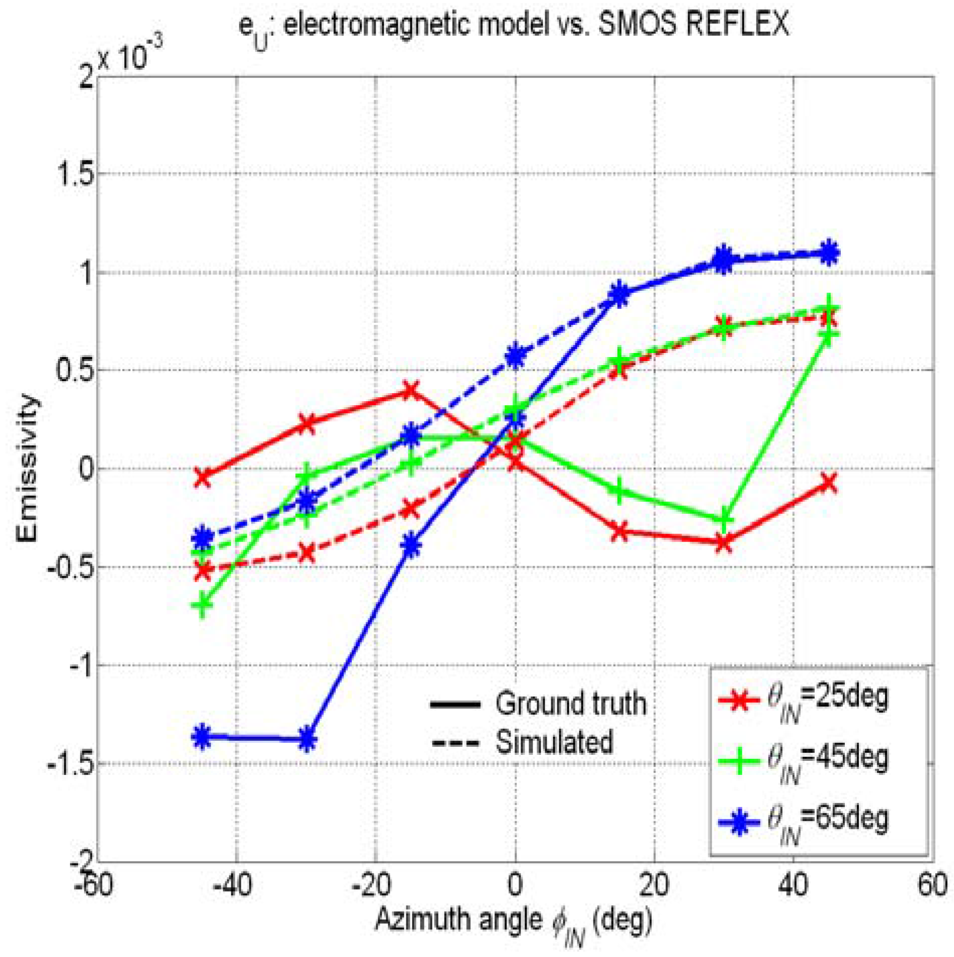
Figure 13 presents the third parameter of the Stokes modified emission vector (
eU) for the same vineyard as a function of the azimuth angle. The third and fourth Stokes elements are measured from the real and imaginary parts of the complex cross-correlation of the electric fields at vertical and horizontal polarizations as in Equation (1) [the third (fourth) Stokes parameter can also be measured as the difference between the brightness temperatures measured at two orthogonal linear (circular) polarizations at +45° and -45° (LHCP and RHCP)].
Solid lines correspond to the measured values in the field experiment, while the dashed lines are simulated values using Equation (6), scaled by a factor equal to 1/30. This empirical factor corresponds to the inverse of the approximate number of grapes per bunch, as if the whole bunch was a single scatterer and not an ensemble of smaller scatterers. While
eh and
ev are dominated by the scattering and attenuation in the branches,
eU seems to be dominated by the scattering in the bunches of grapes, and a clustering factor is needed to account for the random distribution of grapes used in the model (
Section 4.3). Fluctuations in
eU are due to the planting pattern of the vineyard, and both the data and simulations show that
eU is nearly insensitive to soil moisture content.
Figure 13.
Third parameter of the Stokes emission vector (eU) as a function of the azimuth angle (incidence angle = 25, 45 and 65°): experimental data (solid lines) and radiative transfer model computed from Equation (6) (dashed lines) scaled by a clustering factor equal to 1/30 to account for near field effects between grapes. The fourth parameter (eV) is equal to zero.
The magnitude of the measured and simulated fourth Stokes parameter (not shown) is negligible as there are no elements that induce a significant phase shift between the electric fields at horizontal and vertical polarizations.
6. Conclusions
This manuscript has described a complete modified Stokes emission numerical simulator of vegetation-covered soils and its application to the study of the influence of realistic L-systems generated vegetation and soil characteristics on the microwave emission at L-band. The four elements of the modified Stokes emission vector are efficiently computed by numerical integration of the scattering coefficients using analytical expressions for trunks and branches (dielectric cylinders), leaves (flattened dielectric ellipsoids), and grapes (lossy dielectric spheres). To keep the computation time reasonable, multiple scattering and clustering effects have been neglected.
As expected, it is found that the emissivity of the first two Stokes elements (eh and ev) is dominated by the soil moisture content, which impacts through changes in the dielectric constant.
The impact of the vegetation layer on the total emissivity (albedo and attenuation) is dominated by the branch volume, whereas it is almost insensitive to the vegetation type and geometry, and the effect of the tree trunk and leaves is very small. The agreement between measurements and simulations is very satisfactory for the emissivity at vertical polarization. At horizontal polarization though, the simple soil emission models currently used prevent the combined soil + vegetation model to correctly follow the measured emissivity trend, since the bare soil emission model decreases too rapidly with increasing incidence angles. Both the albedo and the vegetation attenuation, previously obtained by fitting the
τ-ω model to the experimental data [
5] agree well with the simulated values.
For a soil surface characterized by a zero-mean Gaussian slopes’ pdf, the average emissivity of the third and fourth Stokes parameters is zero. However, for the vines scenario the predicted eU is overestimated due to the random distribution of grapes used in the model, which neglects the clustering effects that take place in the bunches of grapes. A clustering factor roughly equal to the number of grapes per bunch must be included to adjust simulations and experimental data. On the other hand, within the measurement error level, eV is zero, as confirmed by simulation results.

 ,
, 