Potential Species Distribution of Balsam Fir Based on the Integration of Biophysical Variables Derived with Remote Sensing and Process-Based Methods

Abstract

In this paper we present a framework for modelling potential species distribution (PSD) of balsam fir [bF; Abies balsamea (L.) Mill.] as a function of landscape-level descriptions of: (i) growing degree days (GDD: a temperature related index), (ii) land-surface wetness, (iii) incident photosynthetically active radiation (PAR), and (iv) tree habitat suitability. GDD and land-surface wetness are derived primarily from remote sensing data acquired with the Moderate Resolution Imaging Spectroradiometer (MODIS) sensor on the Terra satellite. PAR is calculated with an existing spatial model of solar radiation. Raster-based calculations of habitat suitability and PSD are obtained by multiplying normalized values of species environmental-response functions (one for each environmental variable) parameterized for balsam fir. As a demonstration of the procedure, we apply the calculations to a high bF-content area in northwest New Brunswick, Canada, at 250-m resolution. Location of medium-to-high habitat suitability values (i.e., >0.50) and actual forests, with >50% bF, matched on average 92% of the time.

1. Introduction

Understanding tree species distribution is essential for the sustainable management of forest landscapes and conservation of biodiversity [1,2,3]. Tree species distribution, occurrence, abundance, and growth are all affected by the same primary factors of temperature, soil water availability, incident solar radiation, and soil geochemical properties [4,5,6,7,8]. Sudden changes in any one of these factors can produce important and unalterable changes in the composition and ecology of landscapes. Specific variables with potential to control actual species distribution include: (i) accumulated growing degree days, (ii) precipitation and redistribution of rainwater or snowmelt as surface or sub-surface flow, (iii) surface desertification (especially in arid to semi-arid regions of the world), (iv) minimum winter temperatures, (v) winter thaw-freeze severity [9], (vi) number of frost-free days, (vii) snow accumulation, (viii) soil acidification, (ix) forest floor thickness, (x) soil composition and compaction, (xi) intra- and inter-species competition, (xii) disturbance regimes [10], and (xiii) time since disturbance.

In order to model tree species distribution, a common approach is to relate biologically-relevant environmental variables to species habitat preferences in GIS [3,5,11,12,13]. However, estimation of biophysical properties for large areas has often been based on the collection of point data and numerical interpolation. In general, the quality of interpolation reflects the quality of the spatial point-data and the interpolation method used. Many interpolation methods (e.g., kriging, inverse distance weighing, natural neighbours, nearest neighbours, triangulation, cubic splines [7,14,15]) are incapable of addressing variation in the target measurements as a function of extrinsic factors, such as, for example, time, changes in elevation, slope, direction of the prevailing wind, distance from the coastline, and overall synoptic conditions, other than the internal relationships contained in the data due to autocorrelation. Some interpolation methods like co-kriging, can establish relationships with some external factors, but this is usually limited to a few co-variates. In general, interpolation by most of these methods produces unrealistic values in areas with poor data coverage (with >20-km separation between observation points; [16]) and with strong underlying physical gradients, such as in mountainous terrain [17]. One solution to improving spatial representation of biophysical variables of landscapes is by using remote sensing (RS) data. RS data provide a near continuous sampling of the earth’s surface at practical spatial resolutions and revisitation intervals.

The use of RS data in species distribution studies is not new. For example, (i) Saatchi et al. [18] employed Moderate Resolution Imaging Spectroradiometer (MODIS)-based estimates of leaf area index and percent tree cover, Quick Scatterometer (QSCAT) backscattering, Shuttle Radar Topography Mission (SRTM)-derived digital elevation model (DEM), and Tropical Rainfall Mapping Mission (TRMM)-based rainfall records to model current tree species distribution in the Amazonian basin; and (ii) Zimmermann et al. [19] combined Landsat ETM+ derived indices (i.e., normalized difference vegetation index (NDVI), green vegetation index, wetness index, and soil brightness index) to model species distribution of rare, early successional, and broadleaf-tree species in Utah, USA. In 2003, Turner et al. [20] predicted the widespread development of mapping techniques of landscape-biophysical conditions with MODIS-sensor acquired data (250-m to 1-km resolution, with a 1 to 2-day revisitation cycle). In previous work we have developed several methods to map the biophysical properties of landscapes relevant to understanding tree species distribution in Atlantic Canada, in particular growing degree days (GDD, a temperature-related index of plant growth; [21]) and temperature-vegetation, land-surface wetness index (TVWI; an indirect measure of soil water content, SWC [22]).

In this paper, we provide a framework for modelling potential species distribution (PSD) of balsam fir [bF; Abies balsamea (L.) Mill] as a function of spatial indices of MODIS-based temperature (by means of GDD) and land-surface moisture (TVWI; [21,22]), and incident photosynthetically active radiation (PAR) simulated with the Landscape Distribution of Soil moisture, Energy, and Temperature (LanDSET) model at 250-m resolution [5,17]. No attempt is made to address forest and landscape-forming dynamics associated with inter- and intra-species competition, forest succession, species invasion and extirpation, and disturbance in our definition of PSD. Description of the methods and their application in assessing habitat suitability and PSD are given in Section 2.2 and Section 2.3. Spatial indices of habitat suitability and PSD are provided here as values ranging between 0 and 1, where 0 coincides with unfavourable site conditions and, thus, low probability of species occurrence, and 1, superior site conditions. As a demonstration of the method, we model habitat suitability and PSD for a bF-dominated region of northwest New Brunswick, Canada, and compare modelled results with the occurrence of high bF-content stands (with >50% bF, by volume) from an existing digital forest-cover map of the region. In this comparison, high bF-content stands are selected to eliminate multi-species effects and the potential masking of relationships between bF occurrence and biophysical characteristics of the landscape. A comparison between PSD and existing bF cover is meaningful in this study because bF, as an aggressive tree species, regenerates very well on its own on appropriate sites. As a result, bF is normally not planted in New Brunswick, except for the production of Christmas trees and for research purposes (D.E. Swift, personal communication, 2009).

2. Methods

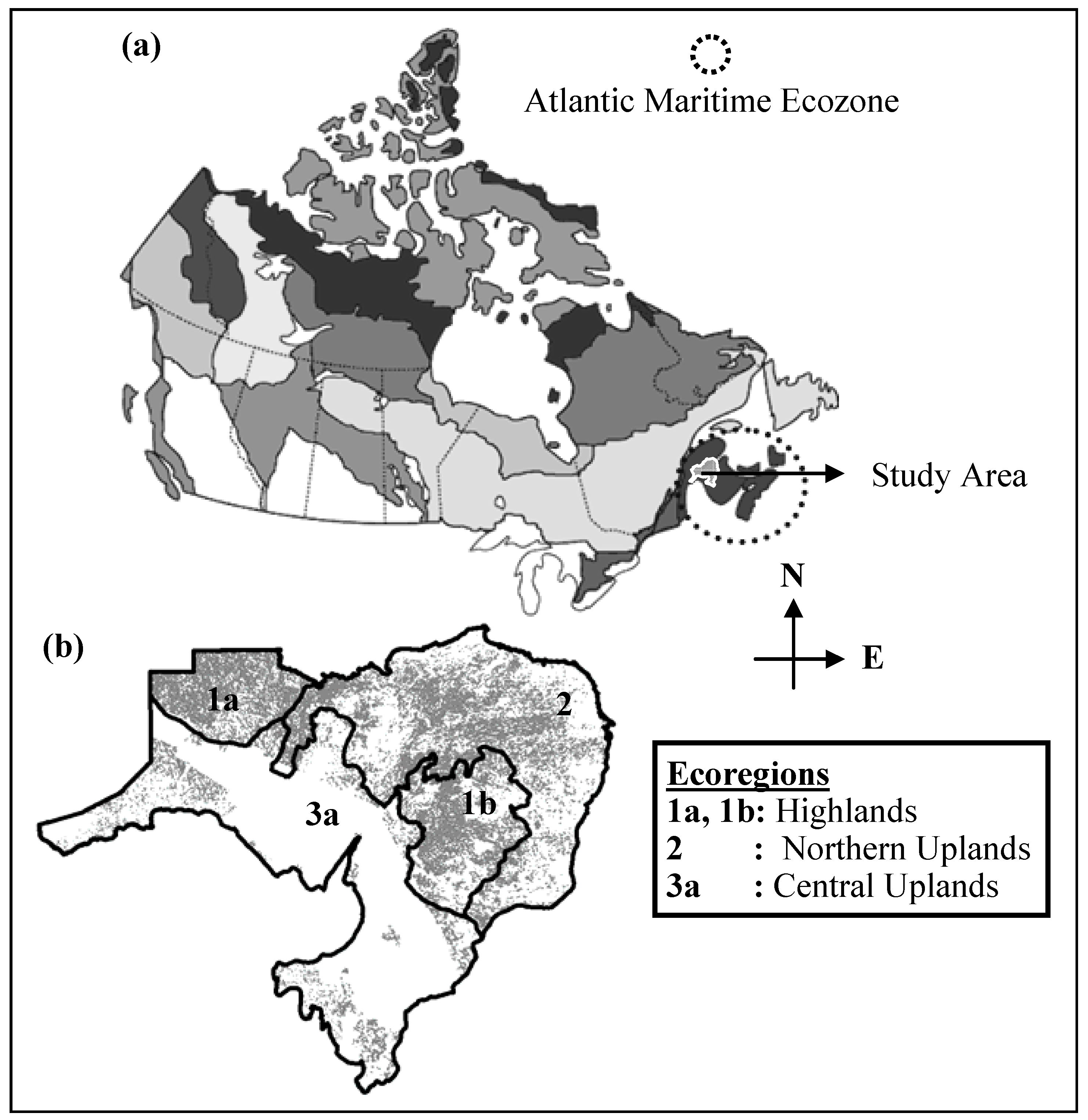
2.1. General Description of Study Area

The study area is in the northwest of the Province of New Brunswick (NB), which falls in the Atlantic Maritime ecozone of eastern Canada (Figure 1a). The area is characterized by temperate evergreen-deciduous mix forest-cover types. Geographically, the area is located between 46^o12'N to 48^o04'N latitude and 65^o38'W to 69^o03'W longitude, and is representative of Highland, Northern Upland, and Central Upland ecoregions of NB (delineated as zones 1a, 1b, 2, and 3a in Figure 1b). Balsam fir is the dominant species, with >50% composition, as identified from aerial photographs [23]. The area is characterized by its variable topography, with elevations ranging from 100 m to 840 m above mean sea level (amsl). The cool-moist climate of the area is largely influenced by the area’s proximity to the Bay of Chaleur in the northeast, movement of continental air masses from the west, and interior highlands. Mean annual temperature and total precipitation in the area varies from 3.5 ^oC to 6.5 ^oC and from 900 mm to 1,500 mm [24].

Figure 1. Location of the study area: (a) in northwest New Brunswick, Canada; (b) extent of high bF-content stands (with >50% bF, by volume) from an existing digital forest-cover map (28120 stands, in all). Forest cover in ecoregion 3a is not available for this study.

Figure 1. Location of the study area: (a) in northwest New Brunswick, Canada; (b) extent of high bF-content stands (with >50% bF, by volume) from an existing digital forest-cover map (28120 stands, in all). Forest cover in ecoregion 3a is not available for this study.

2.2. Data Requirements and Processing

Data employed in this work included (i) RS-based products of GDD and TVWI and estimates of PAR generated with the LanDSET model for the calculation of habitat suitability (HS) and PSD, and (ii) an existing digital forest-cover map (i.e., Forest Inventory Database of the NB Department of Natural Resources, NBDNR; Figure 1b) for species-response equation parameterization (Section 2.3) and validation of PSD.

2.2.1. Growing Degree Days (GDD)

A GDD map at 250-m resolution was previously developed by employing (i) MODIS-based 8-day composites of surface temperature (T_S; at 1-km resolution) and 16-day composites of enhanced vegetation index (EVI; at 250-m resolution) for the April-October period of 2003–2005, (ii) tower-based half-hourly emitted infrared radiation to estimate canopy T_S, and (iii) 30 years (1971–2000 period) average point-estimates of GDD from 101 climate stations from across the Atlantic Maritime ecozone (refer to [21], for greater detail). As an initial step, an empirical relationship was established between mean tower-based estimates of T_S for the MODIS-image acquisition period (i.e., time between 10:30 am and 12:00 pm) and the daily mean T_S. This relationship was subsequently used to estimate daily mean T_S from MODIS-derived values of T_S at 1-km resolution for each 8-day period and GDD using the standard definition, i.e.:

$$GDD={\displaystyle \sum _{i=1}^{i=n}\left({\overline{T}}_a-T_{base}\right)};when{\overline{T}}_a-T_{base}>0$$

(1)

where ${\overline{T}}_a$ is the daily mean air temperature and equal to daily mean T_S [25,26,27], T_base is the threshold temperature, below which plant growth ceases (approximately, 5 ^oC for bF; [21]), and i = 1 represents the start-day and i = n, the end-day of the growing season. Figure 2 demonstrates the relationship between ${\overline{T}}_a$ and daily mean T_S over a bF forest near the southern limit of the study area (Nashwaak Lake, NB). Statistical comparison of values yielded an r²-value = 0.99 and regression equation slope of 1.01 and intercept of 1.98 K. Note that in order to enhance the spatial resolution of the initial GDD map originally at 1-km resolution to 250-m resolution, a data fusion method was developed relating enhanced GDD to seasonally-averaged EVI [21]. Correlation between GDD and EVI was demonstrated to be fairly strong (r² = 0.87). As a result, the application of seasonally-averaged EVI’s to enhance GDD-map resolution was justified [21]. To generate the 30-year average of GDD at 250-m resolution, a constant offset of -511 was applied to reflect the 1971–2000, 30-year normal period [21].

Figure 2. Relation between daily mean ${\overline{T}}_a$ and T_S for the January-October period of 2004 collected over a predominantly bF forest near the southern limit of the study area.

Figure 2. Relation between daily mean ${\overline{T}}_a$ and T_S for the January-October period of 2004 collected over a predominantly bF forest near the southern limit of the study area.

2.2.2. Temperature-Vegetation Wetness Index (TVWI)

A TVWI map at 250-m resolution was developed to address the availability of surface (soil) water [22]. The map was generated by processing 8-day composites of MODIS data of T_S at 1-km resolution and surface reflectance at 250-m resolution for the May-October period of 2003–2005. Surface reflectance values were used to generate NDVI for the area at 250-m resolution. Realistic representation of TVWI across variable terrain required elimination of terrain-induced variations in surface air temperature. To do this, MODIS-based estimates of T_S were converted to potential surface temperature (θ_S) at mean sea level by applying basic meteorological principles of adiabatic compression and a 250-m resolution DEM of the study area in the calculation of vertical atmospheric pressure and air temperature variations in an assumed neutrally-stratified atmosphere [22]. Estimates of TVWI were obtained by interpreting θ_S-NDVI scatterplots generated for each 8-day composite (Figure 3). A long-term average TVWI-map was then produced by averaging all of the individual 8-day TVWI images. TVWI values coinciding with 0 represented the dry sites and 1, the wetter sites. The DEM was generated from 3-arc second SRTM height-data acquired from the National Aeronautics and Space Administration (USA) archives.

Figure 3. Interpretative diagram for TVWI determination (after [22]).

Figure 3. Interpretative diagram for TVWI determination (after [22]).

2.2.3. Photosynthetically Active Radiation (PAR)

In calculating incoming solar radiation and PAR, terrain attributes of: (i) slope; (ii) aspect; (iii) horizon angle; (iv) view factor; and (v) terrain configuration factor were obtained by processing height data from the DEM [5,17]. Incoming solar radiation at the top of the atmosphere was partitioned into its direct and diffused components and each was affected differently as it passed through the assumed cloud-free atmosphere and interacted with the underlying terrain before being summed at the surface [17]. Hourly values generated were then added to provide a growing season total. Available PAR was assumed to be 45% of calculated incoming solar radiation [24]. Finally, PAR was normalized (nPAR = PAR/PAR_max; where PAR_max is the available energy on south-facing slopes) in order that the output from the species-response function for PAR (addressed in Section 2.3) would be constrained between 0 and 1, as would the others.

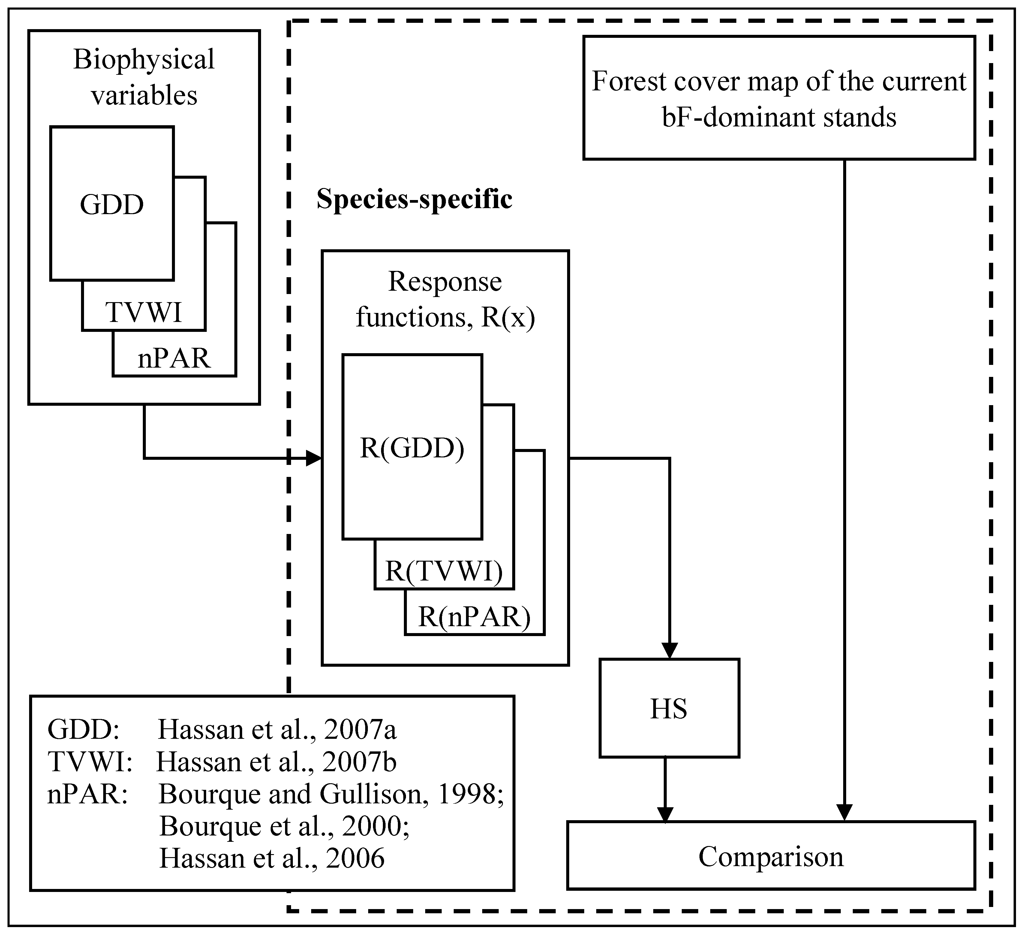
2.3. Modelling of PSD

A conceptual framework for modelling PSD is shown in Figure 4. Development of species-specific environmental response functions for GDD, TVWI, and nPAR followed procedures described in the literature (e.g., [5,28]). TVWI and GDD were both modelled as parabolic functions. A parabolic function for TVWI was legitimate because bF trees grow best in moderately wet soils, and less well in excessively wet or excessively dry soils. We used a linear response function for nPAR. As Barden noted [29], a linear relationship was observed to exist between crop yield and a growing-season integration of PAR in shade-tolerant grass stands. Similar trends were observed in shade-tolerant forests [28].

Figure 4. Conceptual framework for modelling and validating PSD.

Figure 4. Conceptual framework for modelling and validating PSD.

Normalized species-response functions [R(x)] for the individual environmental variables (x) assume the following form:

$$R(GDD)=\frac{4(GDD-GD{D}_{\min })(GD{D}_{\max }-GDD)}{(GD{D}_{\max }-GD{D}_{\min })(GD{D}_{\max }-GD{D}_{\min })}$$

(2)

$$R(TVWI)=\frac{4(TVWI-TVW{I}_{\min })(TVW{I}_{\max }-TVWI)}{(TVW{I}_{\max }-TVW{I}_{\min })(TVW{I}_{\max }-TVW{I}_{\min })}\mathrm{and}$$

(3)

$$R(nPAR)=nPAR.$$

(4)

Equation parameters GDD_min, GDD_max, TVWI_min, and TVWI_max are the minimum and maximum values of GDD and TVWI, respectively. For bF, equation parameters were set according to the values, GDD_min = 700, GDD_max = 2000 (after [30]), TVWI_min = 0.12, and TVWI_max = 0.52. Parameterization of TVWI_min and TVWI_max was based on the occurrence of high bF-content stands described in the digital forest-cover database and associated values of TVWI (Figure 1; [22]).

In a manner similar to the environmental limiting-factor approach of Acevedo et al. [31], the compound effect of the biophysical variables on habitat suitability (HS) and PSD (raster-image of HS) was represented as a product of species environmental-response functions, i.e.,

$$HS=R(GDD)\cdot R(TVWI)\cdot R(nPAR)$$

(5)

3. Results and Discussion

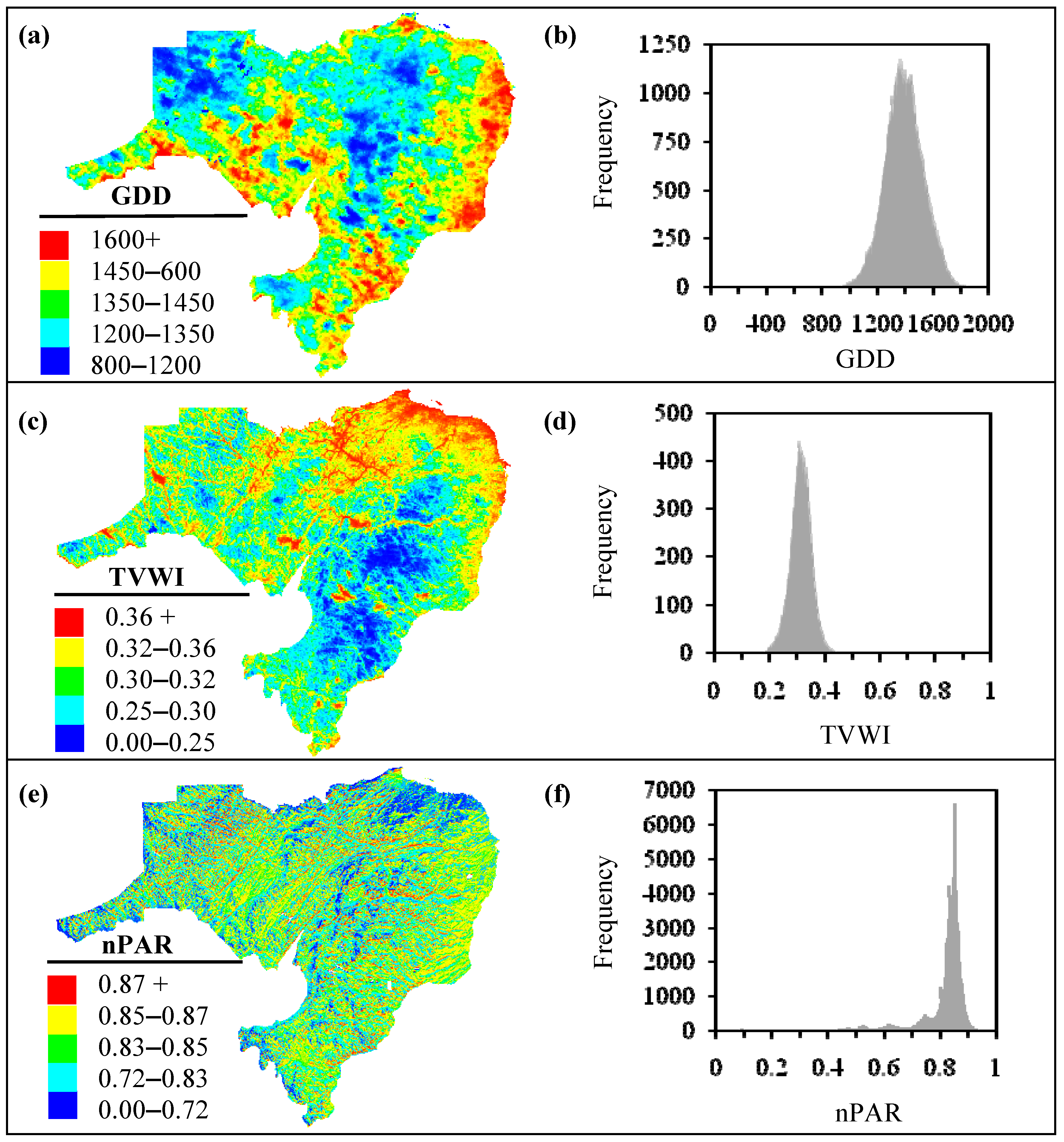
3.1. Biophysical Variables

Figure 5 illustrates both the spatial and frequency distributions for GDD, TVWI, and nPAR. GDD values were observed to be between 950-1800 from the coolest to the warmest locations in the landscape (Figure 5a,b). These values are consistent with values reported by Environment Canada for GDD calculated with a base temperature of 5 ^oC (Canadian Climate Normals for NB, 1971–2000; http://climate.weatheroffice.ec.gc.ca/climate_normals/index_e.html, website last accessed on July 2009). In the case of TVWI (Figure 5c,d), a comparison with LanDSET-calculated SWC [5,17] revealed very similar distributions (r² = 0.96; [22]). A comparison between field-based measurements of PAR and modelled PAR (Figure 5e and Figure 5f) at two forest-sites in NB using LanDSET, also provided reasonable agreement (r² = 0.96; [24]).

3.2. Spatial Distribution of PSD in Comparison to Existing Forest-cover

Figure 6 shows the spatial distribution of modelled HS and PSD for bF in northwestern NB. We summarize PSD patterns in the following way:

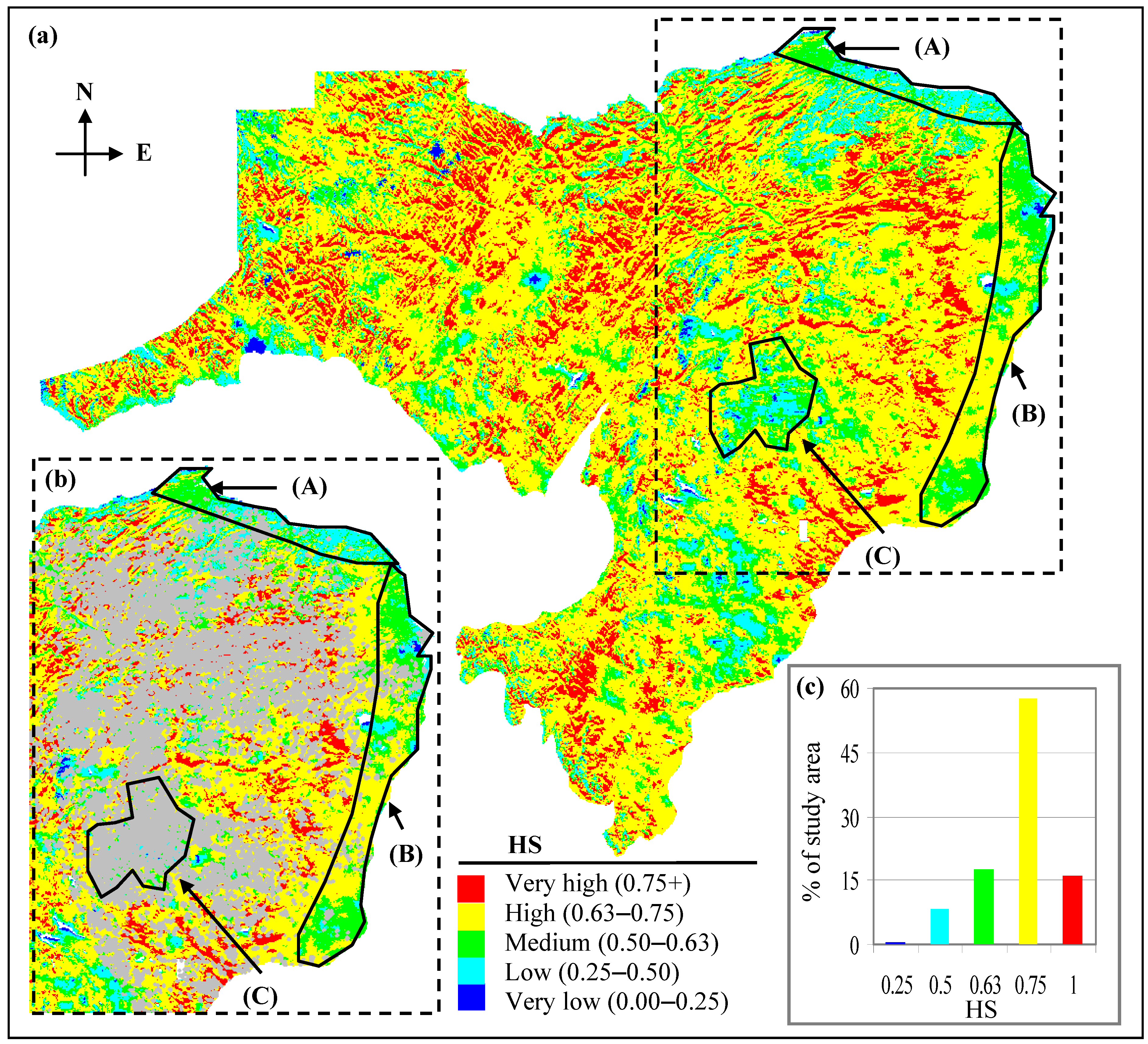
• Polygon A shows an area with low-to-medium HS values (i.e., in between 0.25–0.63; Figure 6a,b). This area is prone to lower PAR, increased TVWI due to physiographic position, and relatively high GDD as a result of the area’s proximity to the Bay of Chaleur to the north. This area most likely provides a better growing environment for temperate, hardwood species. This is consistent with species distribution maps produced by Godin and Roberts [23]. The few bF stands in the area (Figure 6b) support this interpretation.

Figure 5. Spatial and frequency distribution of GDD [(a) and (b)]; TVWI [(c) and (d)]; and nPAR [(e) and (f)].

Figure 5. Spatial and frequency distribution of GDD [(a) and (b)]; TVWI [(c) and (d)]; and nPAR [(e) and (f)].

2.

Polygon B shows an area that is partially affected by a rain shadow produced by the Central Uplands of NB (producing lower TVWI); dominant HS values in the area are in the medium-to-high value range (i.e., 0.50–0.75; Figure 6a,b). However, the lack of bF stands in the area (Figure 6b) contradicts what we would expect with high HS. This may be related to the fact that bF in most of these stands were affected by spruce budworm attack during 1970–1990 [32] and past management activities (D.E. Swift, personal communication, 2009). Currently, bF resides in the understory and is anticipated to become prominent with the release and growth of bF in the understory as the stand nears maturity (D.E. Edwin Swift, personal communication, 2009). Also, high GDDs in the area potentially favour growth of hardwood species, which would tend to out-compete bF, potentially relegating bF (a shade-tolerant species) to the understory.

Figure 6. Spatial distribution of modelled HS and PSD for bF (a); outlined areas A-C are identified to assist with discussion on PSD characteristics in the main body of the paper; bF-dominated stands (light gray polygons; >50% bF) are overlain a portion of the study area (b).

Figure 6. Spatial distribution of modelled HS and PSD for bF (a); outlined areas A-C are identified to assist with discussion on PSD characteristics in the main body of the paper; bF-dominated stands (light gray polygons; >50% bF) are overlain a portion of the study area (b).

3.

Polygon C shows areas with HS mostly in the low-to-medium value range (i.e., 0.25–0.63; Figure 6a,b). The current forest-cover map indicates many bF stands in the area (Figure 6b). This profusion of bF, mostly at elevations >450 m amsl, is indicative of reduced species competition as a result of lower GDD, which typically favour the growth of bF (D.E. Swift, personal communication, 2009), albeit at reduced rates.

4.

Medium-to-very high HS (0.50–1; Figure 6a) predominate the study area (~91% of the landbase; Figure 6c). Moderate-to-low HS (0.25–0.50; Figure 6a,c) are found on about 8% of the area. Poor bF habitat (with HS < 0.25; Figure 6a,c) constitutes <1% of the total land area, and is found mostly in the warmer and wetter areas of the landscape.

An overlay analysis carried out to examine the relationship between high bF-content stands (with >50% bF; Figure 1b) and HS values (Figure 6a) revealed that on average 92% of the stands fell in zones of medium-to-very high HS (>0.50; Table 1).

Table 1. A summary of an overlay analysis of high bF-content stands with respect to modelled HS; “n” is the number of stands falling in each bF-content category (“%”).

Stand bF content (“%”)	Number of stands (n)	“%” of stands by HS range
		<0.5 (Very low-to-low)	>0.5 (Medium-to-very high)
50–60%	11035	6.7%	93.3%
60–70%	9470	7.3%	92.7%
70–80%	4927	9.1%	90.9%
80–90%	1771	11.8%	88.2%
90–100%	886	14.1%	85.9%
100%	31	16.1%	83.9%
50–100%	28120	7.9%	92.1%

Table 1. A summary of an overlay analysis of high bF-content stands with respect to modelled HS; “n” is the number of stands falling in each bF-content category (“%”).

Stand bF content (“%”)	Number of stands (n)	“%” of stands by HS range
		<0.5 (Very low-to-low)	>0.5 (Medium-to-very high)
50–60%	11035	6.7%	93.3%
60–70%	9470	7.3%	92.7%
70–80%	4927	9.1%	90.9%
80–90%	1771	11.8%	88.2%
90–100%	886	14.1%	85.9%
100%	31	16.1%	83.9%
50–100%	28120	7.9%	92.1%

3.3. Future Considerations

In order to enhance the current capacities of PSD modelling in northwestern NB, we need to consider the following issues:

• Ecoregion 3a (Figure 1b) has limited forest cover indicated compared to the other regions as most of the land in that region is owned by private companies, limiting the evaluation of HS and PSD for that area.
• An important site variable, the soil (e.g., [5,12]), is currently not incorporated in the definition of PSD. Existing soil maps are based on geological formations and, as a result, they tend to be unrepresentative at smaller spatial resolutions.
• Implementation of the framework to address other species might require investigating environmental responses for those species (e.g., [5,33]). Although it is reasonable to assume, as a first approximation, that the effect of temperature and SWC can be reasonably represented as parabolic functions; it is likely, however, that the relationships are asymmetrical and vary according to tree species (e.g., temperature optimum), soil texture, and available soil water [34]. Over periods of 30 days or more, the assumption that photosynthesis (and growth) is a linear function of absorbed PAR is realistic, as long as stomatal conductance is not limiting and leaves are present. However, this assumption may be less realistic at shorter time intervals.
• The process of normalization, as applied in northwest NB, should be applied to other biomes in a similar manner (i.e., normalization is biome specific).

3.4. Comparison of PSD Methods

Features of our method that contribute to the field of PSD modelling (e.g., [12,14,15,18,35]) include:

• Currently, many PSD studies use interpolation to derive input surfaces of biophysical variables in the development of PSD maps. In our work, we employ RS data and process-based modelling techniques to eliminate the inherent problems associated with interpolation of sparse data.
• The PSD work of Saatchi et al. explicitly uses RS data [18]. However, predicting the future state of the landscape under scenarios of climate change would be impossible because their methods lack the capability to predict future states. In contrast, our method can be used to predict future PSD of selected tree species (a) by directly incorporating Global Circulation Model (GCM)-projected increases in temperature in the GDD map, and (b) by replacing estimates of TVWI with SWC derived with the soil-hydrology component of LanDSET. Procedures to carry out such work are addressed in a recent paper [36] discussing the effects of climate change on species distribution in the Acadian forest region of eastern Nova Scotia.
• Most studies in PSD modelling are applied at spatial resolutions of 1–10 km [e.g., 12,14,15,35]. As a result, the utility of the information to forest management and wood supply analysis and planning professionals is limited. Our method can generate realistic maps of PSD at 250-m resolution with existing MODIS data and landscape-process modelling techniques.

4. Concluding Remarks

We have established a simple and practical approach to modelling species-specific PSD for bF by integrating spatial descriptions of biophysical variables derived from RS and process modelling techniques for a largely unmonitored region. The use of RS data to derive estimates of potential species distribution (by way of habitat suitability, HS, calculations) at sufficiently small spatial resolutions (250-m) is a unique contribution to forest management. Direct linkage of environmental variables to plant growth by way of environmental-response functions is an element that permits the current work to be extended to investigate tree distribution and, in the future, growth and yield projections under various scenarios of climate change. The modular form of the definition of HS and PSD makes the approach adaptable to other controlling variables (e.g., soil) and plant species, presenting a foundation for monitoring changes in natural systems.

References and Notes

1. Smith, D.M.; Larson, B.C.; Kelty, M.J.; Ashton, P.M.S. The Practice of Silviculture: Applied Forest Ecology, 9th ed.; John Willey & Sons: New York, NY, USA, 1997. [Google Scholar]
2. Austin, M.P. Spatial prediction of species distribution: an interface between ecological theory and statistical modeling. Ecol. Model. 2002, 157, 101–118. [Google Scholar] [CrossRef]
3. Tsoar, A.; Alloche, O.; Steinitz, O.; Rotem, D.; Kadmon, R. A comparative evaluation of presence-only methods for modelling species distribution. Diversity Distrib. 2007, 13, 397–405. [Google Scholar] [CrossRef]
4. Aussenac, G. Interactions between forest stands and microclimate: Ecophysiological aspects and consequences for silviculture. Ann. Forest Sci. 2000, 57, 287–301. [Google Scholar] [CrossRef]
5. Bourque, C.P.-A.; Meng, F.-R.; Gullison, J.J.; Bridgland, J. Biophysical and potential vegetation growth surfaces for a small watershed in northern Cape Breton Island, Nova Scotia, Canada. Can. J. Forest Res. 2000, 30, 1179–1195. [Google Scholar] [CrossRef]
6. Ung, C.-H.; Bernier, P.Y.; Raulier, F.; Fournier, R.A.; Lambert, M.-C.; Regniere, J. Biophysical site indices for shade tolerant and intolerant boreal species. Forest Sci. 2001, 47, 83–95. [Google Scholar]
7. Gustafson, E.J.; Lietz, S.M.; Wright, J.L. Predicting the spatial distribution of aspen growth potential in the upper Great Lakes region. Forest Sci. 2003, 49, 499–508. [Google Scholar]
8. Guisan, A.; Zimmermann, N.E. Predicting habitat distribution in ecology. Ecol. Model. 2000, 135, 147–186. [Google Scholar] [CrossRef]
9. Bourque, C.P.-A.; Cox, R.M.; Allen, D.J.; Arp, P.A.; Meng, F.-R. Spatial extent of winter thaw events in eastern North America: Historical weather records in relation to yellow birch decline. Glob. Change Biol. 2005, 11, 1477–1492. [Google Scholar] [CrossRef]
10. Guisan, A.; Thuiller, W. Predicting species distribution: offering more than simple habitat models. Ecol. Lett. 2005, 8, 993–1009. [Google Scholar] [CrossRef]
11. Gillespie, T.W.; Foody, G.M.; Rocchini, D.; Giorgi, A.P.; Saatchi, S. Measuring and modelling biodiversity from space. Prog. Phys. Geog. 2008, 32, 203–221. [Google Scholar] [CrossRef]
12. McKenny, D.W.; Pedlar, J.H.; Lawrence, K.; Campbell, K.; Hutchinson, M.F. Potential impacts of climate change on the distribution of North American trees. BioScience 2007, 57, 939–948. [Google Scholar] [CrossRef]
13. McKenny, D.W.; Price, D.; Papadapol, P.; Siltanen, M.; Lawrence, K. High-Resolution Climate Change Scenarios for North America. Sault Ste. Marie (Canada): Natural Resources Canada, Front Line Technical Note No. 107; 2006. [Google Scholar]
14. Latta, G.; Temesgen, H.; Barrett, T.M. Mapping and imputing potential productivity of Pacific Northwest forests using climate variables. Can. J. Forest Res. 2009, 39, 1197–1207. [Google Scholar] [CrossRef]
15. Monserud, R.A.; Yang, Y.; Huang, S.; Tchebakova, N. Potential change in lodgepole pine site index and distribution under climatic change in Alberta. Can. J. Forest Res. 2008, 38, 343–352. [Google Scholar] [CrossRef]
16. Peng, G.; Li, J.; Chen, Y.; Norizan, A.P.; Tay, L. High-resolution surface relative humidity computation using MODIS image in Peninsular Malaysia. Chin. Geog. Sci. 2006, 16, 260–264. [Google Scholar] [CrossRef]
17. Bourque, C.P.-A.; Gullison, J.J. A technique to predict hourly potential solar radiation and temperature for a mostly unmonitored area in the Cape Breton Highlands. Can. J. Soil Sci. 1998, 78, 409–420. [Google Scholar] [CrossRef]
18. Saatchi, S.; Buermann, W.; ter Steege, H.; Mori, S.; Smith, T.B. Modeling distribution of Amazonian tree species and diversity using remote sensing measurements. Remote Sens. Environ. 2008, 112, 2000–2017. [Google Scholar] [CrossRef]
19. Zimmermann, N.E.; Moisen, G.G.; Edwards Jr., T.C.; Frescino, T.S.; Blackard, J.A. Remote sensing-based predictors improve distribution models of rare, early successional and broadleaf tree species in Utah. J. Appl. Ecol. 2007, 44, 1057–1067. [Google Scholar] [CrossRef] [PubMed]
20. Turner, W.; Spector, S.; Gardiner, N.; Fladeland, M.; Sterling, E.; Steininger, M. Remote sensing for biodiversity science and conservation. Trends Ecol. Evol. 2003, 18, 306–314. [Google Scholar] [CrossRef]
21. Hassan, Q.K.; Bourque, C.P.-A.; Meng, F.-R.; Richards, W. Spatial mapping of growing degree days: An application of MODIS-based surface temperatures and enhanced vegetation index. J. Appl. Remote Sens. 2007a, 1, 013511:1–013511:12. [Google Scholar] [CrossRef]
22. Hassan, Q.K.; Bourque, C.P.-A.; Meng, F.-R.; Cox, R.M. A wetness index using terrain-corrected surface temperature and normalized difference vegetation index: An evaluation of its use in a humid forest-dominated region of eastern Canada. Sensors 2007b, 7, 2028–2048. [Google Scholar] [CrossRef]
23. Godin, B.; Roberts, M.R. Part I. Ecological Land Classification for New Brunswick: The Ecoprovince, Ecoregion and Ecodistrict Levels [Unpublished report], On file with Provincial Legislative Library, Fredericton, New Brunswick, Canada, Mimeographed, 1994.
24. Hassan, Q.K.; Bourque, C.P.-A.; Meng, F.-R. Estimation of daytime net ecosystem CO2 exchange over balsam fir forests in eastern Canada: Combining averaged tower-based flux measurements with remotely sensed MODIS data. Can. J. Remote Sens. 2006, 32, 405–416. [Google Scholar] [CrossRef]
25. Hassan, Q.K.; Bourque, C.P.-A. Estimating daily evapotranspiration for forests in Altantic Maritime Canada: application of MODIS imagery. In Proceeding ASPRS, Reno, Nevada, USA, May 1-5, 2006. (CD-ROM unpaginated).
26. Sabins, F.F. Remote Sensing Principles and Interpretation, 3rd ed.; W.H. Freeman and Company: New York, NY, USA, 1997. [Google Scholar]
27. Short, N.M. Remote Sensing Tutorial. Available at: http://rst.gsfc.nasa.gov/ (website last accessed August 13, 2009).
28. Shugart, H.H.; Smith, T.M. A review of forest patch models and their application to global change research. Clim. Change 1996, 34, 131–153. [Google Scholar] [CrossRef]
29. Barden, L.S. The linear relation between stand yield and integrated light in a shade-adapted annual grass. B. Torrey Bot. Club 1996, 123, 122–125. [Google Scholar] [CrossRef]
30. Smith, M.J. An Examination of Forest Succession in the Cape Breton Highlands of Nova Scotia. M.Sc. Thesis, University of New Brunswick, Fredericton, 1998. [Google Scholar]
31. Acevedo, M.F.; Urban, D.L.; Ablan, M. Transition and gap models of forest dynamics. Ecol. Appl. 1995, 5, 1040–1055. [Google Scholar] [CrossRef]
32. Taylor, S.L.; MacLean, D.A. Rate and causes of decline of mature and overmature balsam fir and spruce stands in New Brunswick, Canada. Can. J. Forest Res. 2005, 35, 2479–2490. [Google Scholar] [CrossRef]
33. Austin, M.P.; Nicholls, A.O.; Doherty, M.D.; Meyers, J.A. Determining species response functions to an environmental gradient by means of a β-function. J. Veg. Sci. 1994, 5, 215–228. [Google Scholar] [CrossRef]
34. Landsberg, J.J.; Waring, R.H.; Coops, N.C. Performance of the forest productivity model 3-PG applied to a wide range of forest types. Forest Ecol. Manage. 2003, 172, 199–214. [Google Scholar] [CrossRef]
35. Iverson, L.R.; Schwartz, M.W.; Prasad, A.M. Potential colonization of newly available tree-species habitat under climate change: An analysis for five eastern US species. Landscape Ecol. 2004, 19, 787–799. [Google Scholar] [CrossRef]
36. Bourque, C.P.-A.; Hassan, Q.K. Projected impacts of climate change on species distribution in the Acadian forest region of eastern Nova Scotia. Forest. Chron. 2008, 84, 553–557. [Google Scholar] [CrossRef]