Article

Evaluation and Normalization of Cloud Obscuration Related BRDF Effects in Field Spectroscopy

1
M3 BIORES, K.U. Leuven, de Croylaan 34, 3001 Leuven, Belgium
2
Division of Crop Biotechnics, K.U. Leuven, Kasteelpark Arenberg 13, 3001 Leuven, Belgium
*
Author to whom correspondence should be addressed.
Remote Sens. 2009, 1(3), 496-518; https://doi.org/10.3390/rs1030496
Submission received: 1 July 2009 / Revised: 7 August 2009 / Accepted: 11 August 2009 / Published: 25 August 2009

Abstract

:
The impact of target bidirectional reflectance in dual field of view spectroscopy was described and quantified using field measurements and ray-tracing simulations. A data-driven normalization method was developed to convert reflectance factors under cloud obscured conditions into clear sky reflectance by decomposing the target bidirectional reflectance into an isotropic target-specific component and a group-specific bidirectional component. An evaluation on tree, grass and gravel targets suggests a reduction in relative reflectance error obtained by normalization from 15% to less than 5% between 400 and 1800 nm. At higher wavelengths a decreased signal-to-noise ratio increases the errors.

1. Introduction

During the last decades, field spectroscopy has become an established technique for characterizing reflectance of surfaces in situ, for supporting calibration of airborne and satellite sensors (vicarious calibration) and for providing a means of up-scaling data from small surfaces such as leaves, branches and stones to composite scenes such as canopies and ultimately to pixels [1]. The comparably small footprint of spectroradiometers combined with their high spectral resolution enables a precise characterization of an object’s reflectance, without signal deterioration due to atmospheric interactions of the reflected radiance. This higher detail comes at the expense of significantly larger efforts required to establish field datasets. Since single field of view reflectance spectroscopy is based on taking the ratio of sequentially measured target radiance to whitepanel radiance, stable illumination conditions are imperative, which can only be guaranteed under cloudless conditions [2, 3]. Unfortunately, occurrence of such necessary conditions for many regions in the world is subject to seasonality and the dominant sky type may include various amounts of cloud cover (the fraction of the sky hemisphere covered by clouds) and cloud obscuration (the optical depth of the cloud layer obscuring the solar disk and the surrounding corona). Even at visually optimal conditions, measurements can still be deteriorated due to optically thin cirrus clouds passing before the sun disk [4]. While single date dataset collections may permit waiting for optimal conditions, the establishment of time series does not offer such flexibility. In single field of view spectroscopy, often (linear) interpolations are made of the target radiance before and after a set of target scans to account for smoothly varying irradiance such as that due to varying solar zenith angle at clear sky conditions [5]. This interpolation technique, however, can hardly be applied to account for the typically rapid, unpredictable and nonlinear changes in irradiance caused by cloud obscuration. To alleviate these restrictions, dual field of view (DFOV) methods have been designed that rely on the simultaneous measurement of reference and target providing more precise field spectra than results collected using a single-beam mode [3]. Different DFOV implementations have been developed, either by implementing into a single instrument an oscillating shutter or mirror to interleave signals from target and reference or by simultaneously triggering scans of two individual instruments [6]. In both designs, the reference measurement may be either the radiance of a reference panel (bi-conical) or the irradiance obtained by a cosine receptor (cos-conical). For dual instrument designs, intercalibration functions (ICF) are implemented to account for differences in spectral response of both sensors. Research by [6] demonstrated that ICFs depend on the irradiance spectrum and are therefore best established under field conditions approximating those of the target measurements. The significant additional expense of a second spectroradiometer for DFOV measurements has lead to the development of techniques for estimating the irradiance spectrum by only sampling a limited number of fixed wavelength bands using a much simpler filter-based radiometer [5, 7].
Although DFOV techniques can successfully overcome errors caused by varying irradiance, cloud obscuration also causes an increase in incident light scattering. As a consequence, the diffuse to direct ratio of incident light as well as the angular distribution of diffuse light will be altered. The impact of this phenomenon may be limited for light and invisible cirrus clouds under which circumstances DFOV spectroscopy is commonly applied. For obscurations by optically thicker cloud types such as cumulus and stratus clouds, the irradiance distribution will be significantly altered, causing a different sampling of the target’s bidirectional reflectance distribution function (BRDF) and consequently different values of measured reflectance (hereafter named reflectance factor) for most surfaces [8, 9]. Most structured earth surfaces are known to exhibit different amounts of backscatter (soil, vegetation) and/or forward scattering (water bodies). Moreover, also the non-Lambertian behavior of commonly used reference panels such as Spectralon material (Labsphere Inc.) has been well investigated [10, 11, 12]. When taking the ratio of target radiance to reference radiance to obtain re?ectance factors, target and reference panel BRDF effects may either compensate or reinforce each other. A cos-conical configuration can suffer from analogous issues as many commercially available cosine diffusers are based on spectroradiometer fore-optics exhibiting a sub-optimal cosine response [13]. An additional restriction in DFOV under severely obscured conditions is the reduced irradiance resulting in a reduced signal-to-noise ratio (SNR) of the measurements.
The objectives of this research are:
to gain better insights in the mechanisms in which different levels of cloud obscuration affect DFOV spectroscopy. More specifically, the focus will be put on the effects of decreased irradiance (noise level) and target/whitepanel BRDF.
to evaluate whether, for measurement series over similar targets, the target BRDF can be decomposed into an isotropic target-specific component and a group-specific bidirectional component.
to use this decomposition for developing a data-driven normalization procedure for converting, by means of an initial dataset obtained from a representative target, measured reflectance factors into reproducible reflectance measures, independent of cloud obscuration.
The theoretical background section presents the processing of DFOV measurements and the calculation of SNR using error propagation theory. Expressions for quantifying BRDF effects are derived and a normalization procedure is developed. Evaluation of BRDF effects and the normalization procedure relies on both reference data obtained over Citrus canopy, grass sod and gravel targets with DFOV spectroscopy and on hyperspectral ray-tracing data.

2. Theoretical Background

In the first section, the use of instrument intercalibration is discussed. Subsequently, three major effects of cloud obscuration on incident light are considered: (i) the decrease in the total amount of transmitted irradiance due to scattering and absorption by cloud particles, (ii) an increase in the fraction of diffuse light due to a higher amount of scattering and (iii) a different angular distribution of the diffuse light. Finally, a normalization procedure for the second and third effect is developed.

2.1. Overview of Radiometric Units

Table 1 lists a description of the radiometric symbols and units used in this work. For a complete description, we refer to standard works in remote sensing such as [14].
Table 1. List of radiometric symbols and units.
SymbolNameUnits
Lradiance W m - 2 s r - 1
L ( λ ) spectral radiance W m - 2 s r - 1 n m - 1
Eirradiance W m - 2
E ( λ ) spectral irradiance W m - 2 n m - 1
fBRDF or bidirectional reflectance s r - 1
ρreflectance factor-
γfraction of direct irradiance-

2.2. Processing of Dual Field of View Measurements

In DFOV spectroscopy, measurements are made with two identical instruments, one measuring the radiance of a reference whitepanel ( L r e f ) which is used as a surrogate for total incident irradiance [15], and the other measuring the target’s radiance ( L t a r ). The resulting absolute reflectance factor ( ρ t a r ) after correcting for the reference panel reflectance ( ρ r e f ) is:
ρ t a r ( λ ) = L t a r ( λ ) L r e f ( λ ) ρ r e f ( λ )
in which λ represents the wavelength (nm). Generally, both instruments are not completely identical and measure slight differences in radiance due to small errors in calibration or small waveband shifts. Without correction, the resulting spectra can exhibit significant noise levels and therefore intercalibration functions are often applied [6, 16]. Instrument intercalibration is obtained by measuring the radiance with both instruments of a constant intercalibration surface ( L i c ) illuminated with a stable light source. The reflectance factor is then multiplied with an wavelength specific intercalibration term, I C ( λ ) , that equals the ratio of both instruments measured radiances. Although in this form, the intercalibration appears as a constant spectrum, its value depends on the shape of the irradiance spectrum [6]. Intercalibration functions are thus best established under illumination conditions approximating those under which the field measurements are collected. To reduce notational complexity, intercalibration is omitted in subsequent formulations, although it is consistently applied when processing real measurements.

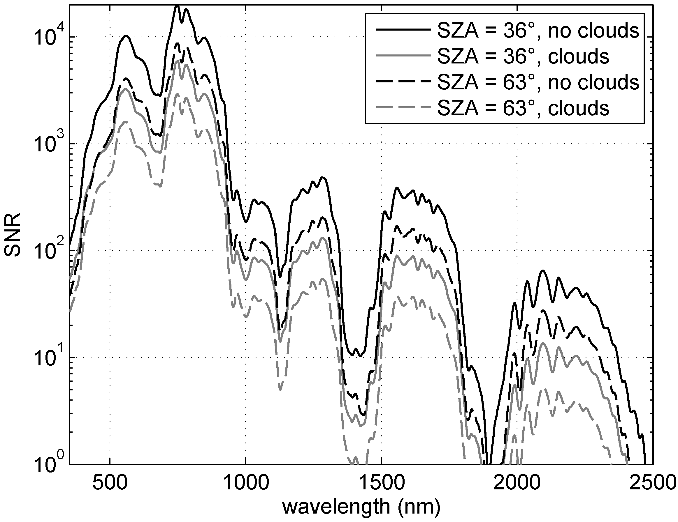
2.3. Impact of Cloud Obscuration on Signal Noise

Spectroradiometers exhibit different sensitivities along the wavelength spectrum they are designed to measure. Measurement noise is commonly expressed as noise equivalent radiance ( N E R ) and is measured as the standard deviation in radiance of a sufficiently large number of 1 s scans over a target illuminated with a perfectly stable light source [2]. For a given measured radiance of a target L t a r , the signal to noise ratio (SNR) in radiance units can be expressed as:
S N R ( λ ) t a r , r a d = L t a r ( λ ) N E R ( λ ) T
with T being the scan time in seconds, expressing a decrease in noise level according to the square root law (of sample size). Since the property of interest is target reflectance, the SNR of the reflectance factor can be expressed using the standard error rule of a ratio:
S N R ( λ ) r e f l = 1 1 S N R ( λ ) t a r , r a d 2 + 1 S N R ( λ ) W P , r a d 2
with S N R W P , r a d as the signal-to-noise ratio of the whitepanel measured with the same illumination. Equation 3 can be used to estimate SNR of an intended measurement series if approximations of the irradiance spectrum and target reflectance are available.

2.4. BRDF Effects Caused by Illumination Conditions

This section discusses the impact of cloud cover on the fraction of diffuse irradiance and the angular distribution of diffuse light. Differences in cloud cover during a measurement series will cause a different sampling of the target’s BRDF and result in different measured reflectance values. In addition, the non-Lambertian BRDF of whitepanels should be taken into account [16]. Both statements can be explained by expressing target and reference surface radiance as functions of the direct and diffuse irradiance components. For isotropic surfaces, where the BRDF only depends on the relative difference between viewing ( φ v ) and illumination azimuths ( φ i ), the radiance of a target can be expressed as:
L t a r = E d i r f t a r θ i , θ v , φ i - φ v + 0 2 π 0 π / 2 f t a r θ , θ v , φ - φ v L d i f ( θ , φ i ) cos θ sin θ d θ d φ
with θ i and θ v the illumination and viewing zenith angles, f t a r the BRDF of the target surface, E d i r the direct (projected) irradiance and L d i f the angular distribution of the diffuse irradiance (skylight) under specific illumination conditions (i). Note that BRDF (f) and reflectance factor (ρ) are related by a constant, i.e., ρ = π f t a r . Equation 4 can also be used to obtain the reference panel radiance ( L r e f ) when replacing f t a r by f r e f , the reference panel BRDF. For nadir viewing angles, Equation 1 can be converted using basic mathematical operations into (see appendix section):
ρ t a r n a d i r = γ d i r f t a r θ i , 0 + ( 1 - γ d i r ) 0 π / 2 f t a r θ , 0 w θ i d θ γ d i r f r e f θ i , 0 + ( 1 - γ d i r ) 0 π / 2 f r e f θ , 0 w θ i d θ ρ r e f n a d i r
in which γ d i r is the fraction of direct irradiance on a horizontal surface and w θ i expresses the distribution of diffuse irradiance under specific illumination conditions (i) as a weighting function. This expression no longer depends on absolute (radiometric) measures of light flux. Different (polynomial) expressions exist to describe the BRDF of Spectralon material [10, 17, 18] that is commonly used as the reference surface, so we assume f r e f to be known. Its impact on reflectance factors measured under obscured conditions is discussed in Section 4.3. The other parameters are harder to determine since they depend on the BRDF shape of the (unknown) target and on the specific illumination conditions at the time of measurement.
All variables also depend on wavelength. For f t a r and f r e f this is inherent to the BRDF itself. γ d i r depends on the amount of scattering by air and cloud particles and therefore increases with increasing wavelength (Rayleigh scattering) while water absorption regions also impact its magnitude [19]. Wavelength dependencies of γ d i r and the weight function (w) are discussed in Section 4.2.

2.5. Normalization Factor for Dual-Beam BRDF Effects

In this section a normalization strategy is developed to convert the measurements from a dataset with different levels of cloud obscuration to quasi clear sky reflectance. The normalization is data-driven without the requirement of additional data on atmospheric conditions or reference or target BRDF shape and relies on the similarity in BRDF shape of similarly structured targets. The term “quasi clear sky” (QCS) will be used for prevailing partly cloudy conditions with no clouds obscuring the solar disk or the surrounding corona, i.e., the CIE white-blue sky with distinct solar corona (type V.4) [20]. “Clear sky” (CS) then refers to a cloudless sky as defined in the CIE Standard Clear Sky (type IV.4). The similarity between both sky types, with respect to the normalization procedure, is discussed in Section 4.2.
The function f t a r in Equations 4 and 5 describes the target bidirectional reflectance under different illumination conditions and is the key factor in obtaining QCS reflectance factors. When no multi-angular observations are available, f t a r cannot be derived from field spectroscopy data. Prior knowledge or assumptions are thus required. This is achieved by decomposing f t a r for an arbitrary viewing and illumination geometry into the product of (i) a target specific reflectance factor, ρ ¯ t a r ( λ ) independent of viewing and illumination geometry and (ii) a bidirectional component, κ t a r ( λ , θ i , θ v , φ i - φ v ) determined by the general structure of the target type and describing the relative shape of the BRDF. The shape of κ t a r as a function of viewing and illumination angles should thus be approximately equal for different targets of the same type. The decomposition described here is thus based on the same principle as the kernel-driven MODIS Albedo product for sparse angular sampling [21]. For nadir viewing, it allows the retrieval of ρ ¯ t a r ( λ ) from Equation 5 if κ t a r , κ r e f , γ d i r , w and f r e f are known.
During a short measurement series with constant solar elevation under partly cloudy conditions over a constant target, variations in cloud obscuration (COD) are considered to be the dominant atmospheric parameter influencing the angular distribution of incident light (w) and the fraction of direct incident light ( γ d i r ). Short-term (hourly) variations in other atmospheric parameters such as atmospheric haze (expressed as atmosphere optical depth or AOD) are not considered here. Research by [22] indicates that although diurnal fluctuations in AOD can be considerable, hourly fluctuations are smooth (as opposed to sudden changes in COD) and limited in magnitude. From Equation 5 can now be derived that the ratio of two reflectances obtained form the same target, one measured with a certain level of cloud obscuration (COD = x) and the other with a (quasi) clear sky (QCS or COD = 0), is no longer a function (g) of the target specific reflectance factor ρ ¯ t a r . This ratio only depends on the bidirectional shape parameters ( κ r e f and κ t a r ) and illumination conditions ( θ i , γ d i r and w):
ρ t a r x ( λ ) ρ t a r Q C S ( λ ) = g γ d i r Q C S , w Q C S , γ d i r x , w x θ i , κ t a r , κ r e f , λ
The function g, for specified values of θ i , κ t a r and κ r e f , can be experimentally determined (e.g., using quadratic regression) for each wavelength (λ) using only reflectance factors obtained over a constant target for a range of COD values (see Figure 5 for examples).
For practical DFOV applications however, it is preferred to reformulate g as a function of incident radiance (L) or irradiance (E) quantities that, unlike γ d i r or w, are automatically measured by the spectroradiometer making the reference measurements. Simulations with atmospheric radiative transfer models (see also Section 4.2) demonstrate that, with increasing levels (x) of COD, the total irradiance ( E t o t x ) monotonically decreases while γ d i r x also monotonically decreases and w x evolves towards a fixed distribution. Under such conditions a unique relationship exists between E t o t x on one hand and γ d i r x and w x on the other hand. Consequently Equation 6 can be reformulated as:
ρ t a r x ( λ ) ρ t a r Q C S ( λ ) = g E t o t x E t o t Q C S θ i , κ t a r , κ r e f , λ
The technique described here is analogous to empirical relationships established to derive atmospheric properties such as turbidity and clear sky index from relative total irradiance [23]. As an easier alternative, measurements may be discretized into a “quasi clear sky set” containing scans with no obscuration and an “obscured sky set” containing scans with full obscuration (high values of COD), turning g into a constant spectrum. Once determined for a single target, g can be applied as a normalization factor ( n f ) to convert reflectance factors of other targets with a similar structure (e.g., trees of the same species, stand and age class) measured under cloud obscuration (but equal solar elevation angle) into QCS reflectance ( ρ t a r Q C S ). As a consequence, the proposed normalization procedure does not require a full characterization of the target BRDF nor a full description of κ t a r , but rather of a group of targets by a n f derived under equal illumination conditions. This n f may be obtained at the start of a field dataset collection by fixing the target spectroradiometer over a representative target such as a tree crown or a part of a grass sod, and simultaneously measuring reflectance factors and spectral irradiance under varying levels of clouds for approximately 15 to 30 minutes. Porting an established n f to different measurement days is possible as long as illumination conditions, such as cloud type and solar elevation, are almost equal.

3. Materials and Methods

3.1. Field Measurements

Five hyperspectral field datasets were collected in Leuven, Belgium (50°52’N, 4°42’E) over three different targets: a grass sod (Lolium perenne L.) on a loamy soil, potted Citrus trees placed on a loamy soil and gravel. Solar zenith angles (SZA) during measurement time range between 36° and 63°. Yearly minimal and maximal SZA at solar noon at the measurement site are 27° and 74°. All datasets were collected under a partly cloudy sky (CIE types IV.2, IV.3 and IV.4) with different levels of cumulus clouds as such that each set contains several clouds obscuring the solar disk. The length of each series was restricted to approximately 40 minutes to minimize effects in impact of changing solar elevation. Table 2 summarizes the measurement conditions, including the approximate range of total irradiance. Total irradiance was estimated by converting the measured whitepanel radiance into irradiance. Two independent dataset (different trees of equal cultivar, age and phenology) were obtained for Citrus under comparable illumination conditions. The first is intended for derivation of the normalization factor ( n f ) while the second set is intended to test the normalization procedure.
Table 2. Overview of measurement conditions and targets for field measurements.
targetday, timesolar zenith (°)min. irradiance ( W m - 2 )max. irradiance ( W m - 2 )
Citrus tree canopies (set 1)8-24-2008, 13h1041°158886
Citrus tree canopies (set 2)30-4-2009, 13h0036°190859
grass sod (0.05 m height)9-10-2008, 14h0046°160752
grass sod (0.05 m height)9-10-2008, 17h0063°136385
gravel9-11-2008, 14h0046°203785
Field measurements were made with two Spectra-Vista HR-1024 spectroradiometers with spectral resolutions of 3.5 nm between 350 and 1,000 nm, 8.5 nm between 1,000 and 1,850 nm and 6.5 nm between 1,850 and 2,500 nm. A reference instrument with a 4° FOV fore-optic was mounted on a tripod over a Spectralon whitepanel placed 0.5 m below the sensor lens. The second target instrument with a 25° FOV fore-optic was mounted on a second tripod at 1.7 m height for measurements of the grass sod and gravel surfaces. For the tree canopies, the instrument was attached with a fixture onto a scaffold at 3.5 m height. The larger spot size of the 25° FOV fore-optic, approximately 0.08 m² at 1.5 m distance [24], assures a more representative sampling of ground targets while the 4° FOV fore-optic assures a correct focusing on the center of the whitepanel. Per series between 30 and 50 scans were made, each of 10 s length with varying levels of obscuration and overall sky cloud cover. Both instruments were manually triggered to start measuring at exactly the same time (less than 0.1 s time difference). During a measurement series, the sensor gain of each instrument was automatically determined at the start of each individual scan. This assured optimal signal-to-noise ratios at the light intensity level of each individual scan. Measurements where light intensity substantially increased during the scan time resulted in saturation effects in the detectors and those saturated spectra were filtered during data preprocessing. All spectra were collected in radiance mode ( W m - 2 s r - 1 n m ). For each measurement set, intermediate intercalibration scans were made with both instruments measuring a level Spectralon whitepanel to obtain an ICF under field conditions as suggested by [6].

3.2. Ray Tracing Simulations

Three different virtual targets were constructed: gravel surface, grass sods and Citrus sinensis L. (Osbeck) trees. For each target, measurements were simulated in a ray tracing environment for different solar elevations and atmospheric conditions. The ray tracer, PBRT, is a physically based ray tracer [25] adapted for hyperspectral radiative transfer simulations and validated with the RAMI Online Model Checker [26]. Measurements were simulated from 400 nm to 2,500 nm in 10 nm increments. Per simulation, 250,000 random rays were cast, which guarantees a relative error in reflectance below 0.4% for all wavelengths [27]. Simulations were set up to approximate (but not to equal) field conditions with similar targets, atmospheric conditions and sensors. Since the aim of the simulations was a theoretical analysis of BRDF effects with DFOV sensors for various conditions and targets, no attempt was made to obtain an exact calibration for the specific measurement settings.
A virtual 25° field of view camera was positioned at 5 m height for the tree simulations (3 m above the top-of-canopy) and at 3 m height for the sod and gravel targets. The gravel surface was simulated as a simple flat surface using the Hapke-Jacquemoud soil BRDF model [28] and bidirectional coefficients for pebble surfaces ( h = 0.09 , b 0 = 1.11 , c 0 = 0.53 , b 1 = 0.33 , c 1 = - 0.11 ). The single scattering albedo was obtained by inversion of reflectance spectra collected with a Spectra-Vista HR-1024 spectroradiometer.
The grass sod was simulated as randomly placed disks with a 0.01 m radius, an elevation between 0 and 0.1 m and an erectophile leaf angle distribution as defined in [29]. Grass leaf reflectance and transmittance were simulated as Lambertian surfaces with spectra (Phleum sp.) obtained from the LOPEX dataset [30].
The Citrus tree structures were calibrated on ten Citrus trees in a commercial orchard in Wellington, South-Africa [31]. The calibration procedure is described in [27]. Citrus stem reflectance was Lambertian and leaf reflectance and transmittance were calibrated on measured spectra with the Bousquet microfacets model [32]. The ten calibrated trees used in the simulations comprise a set with large variations in both tree canopy structure (e.g., LAI at tree level ranges from 3.2 to 11) and leaf reflectance (e.g., average leaf chlorophyll content per tree from 47 to 89 μ g c m - 2 ). The underlying soil, identical for each tree, was simulated as a moist loamy soil (coefficients h = 0.09 , b 0 = 1.11 , c 0 = 0.64 , b 1 = 0.18 , c 1 = - 0.05 ) using the Hapke-Jacquemoud BRDF model. An identical inversion procedure on measured spectra was used to obtain the single scattering albedo of a loamy soil (Alfisol). Total direct and diffuse irradiance as well as the angular distribution of diffuse irradiance were simulated with the SBDart atmospheric model [33] for wavelengths from 400 to 2,500 nm (per 10 nm) at an angular resolution of 2° and subsequently implemented as direct and hemispherical (diffuse) light sources in pbrt. Simulations were made for solar zenith angles of 20, 30, 40, 50 and 60° and for ten levels of cloud optical depth (COD) between 0 and 100 at logarithmic increments. Cloud height (4,000 m), cloud thickness (400 m), aerosol optical depth (0.3) and atmospheric water vapor ( 2.5 g c m - 2 ) and ozone ( 0.3 g c m - 2 ) concentrations were fixed at typical values for mid-latitude atmospheric conditions. Cloud cover was simulated as a uniformly overcast sky. In all simulations, the effect of the reference panel BRDF was included using a fourth order polynomial approximation of the panel BRDF as established by [18].

4. Results and Discussion

In the first set of simulations, the impact of the reduced irradiance (signal strength) due to cloud obscuration on the measured SNR is discussed. Subsequently, ray-tracing simulations combined with atmospheric radiative transfer models are used to reproduce BRDF effects of different targets for varying illumination conditions. Results are compared to field collected datasets and recommendations are formulated for optimal measurement conditions. In the last step, the normalization procedure is evaluated on synthetic and real measurements.

4.1. Impact of Cloud Cover on the Signal-to-Noise Ratio

To assess the impact of cloud cover on signal quality, the NER of both spectroradiometers was determined using 20 consecutive 1 s scans. SNR in spectral radiance units ( W m - 2 s r - 1 n m ) was obtained from Equation 2 using measured radiance of a grass sod target for a 10 s scan time (T). Obtained results agree with manufacturer provided instrument specifications. SNRs were calculated for four different illumination conditions consisting of combinations of low (36°) and high (63°) solar zeniths with obscured and non-obscured conditions. Analogously, SNR for the instrument measuring the reference panel were obtained for the same measurement conditions. Both values were combined into the SNR of reflectance (Equation 3) as illustrated in Figure 1, from 350 to 2,500 nm. Although these results are specific for the combination of instrument type, target and illumination conditions being used, it allows to make some general inferences. Due to a low instrument NER in combination with high spectral irradiance, the SNR in the 450–900 nm region is at least one order of magnitude larger than in the higher wavelengths, even for the vegetative target that has a low reflectance in the visible part of the spectrum (VIS, 400–700 nm). For the unfavorable combination of a low zenith angle and obscured illumination, the SNR in this region still exceeds 100. The usability of the 1,000–1,800 nm region is heavily impacted by both solar elevation and cloud thickness. The SNR drops below 10 above 2,000 nm in the case of cloud obscuration. DFOV spectroscopy applied under cloud obscured conditions will thus require longer measurement times or a larger number of scans from the same target to achieve equal SNR levels as compared to clear sky conditions. Alternatively broader spectral regions around the atmospheric water absorption regions or even the entire 1,800–2,500 nm region may need to be excluded from analysis. This analysis indicates that DFOV time series can be established even with low illumination conditions for the monitoring of chlorosis-related stresses such as nitrogen deficiencies that show up in the VIS spectrum [34] and canopy structure changes that are most pronounced in the near-infrared (NIR) [35]. Monitoring of changes that appear in the short-wave infrared (SWIR) may on the other hand be restricted. Further reductions in noise levels under prevailing atmospheric conditions can be obtained by applying advanced noise filtering techniques [36].
Figure 1. Signal-to-noise ratios for dual FOV measurements using Spectra-Vista HR-1024 instruments and 10 s integration times. Measurements at Leuven, Belgium, 10/9/2008, 14h00 local time (SZA = 36°) and 17h00 local time (SZA = 63°).
Remotesensing 01 00496 g001

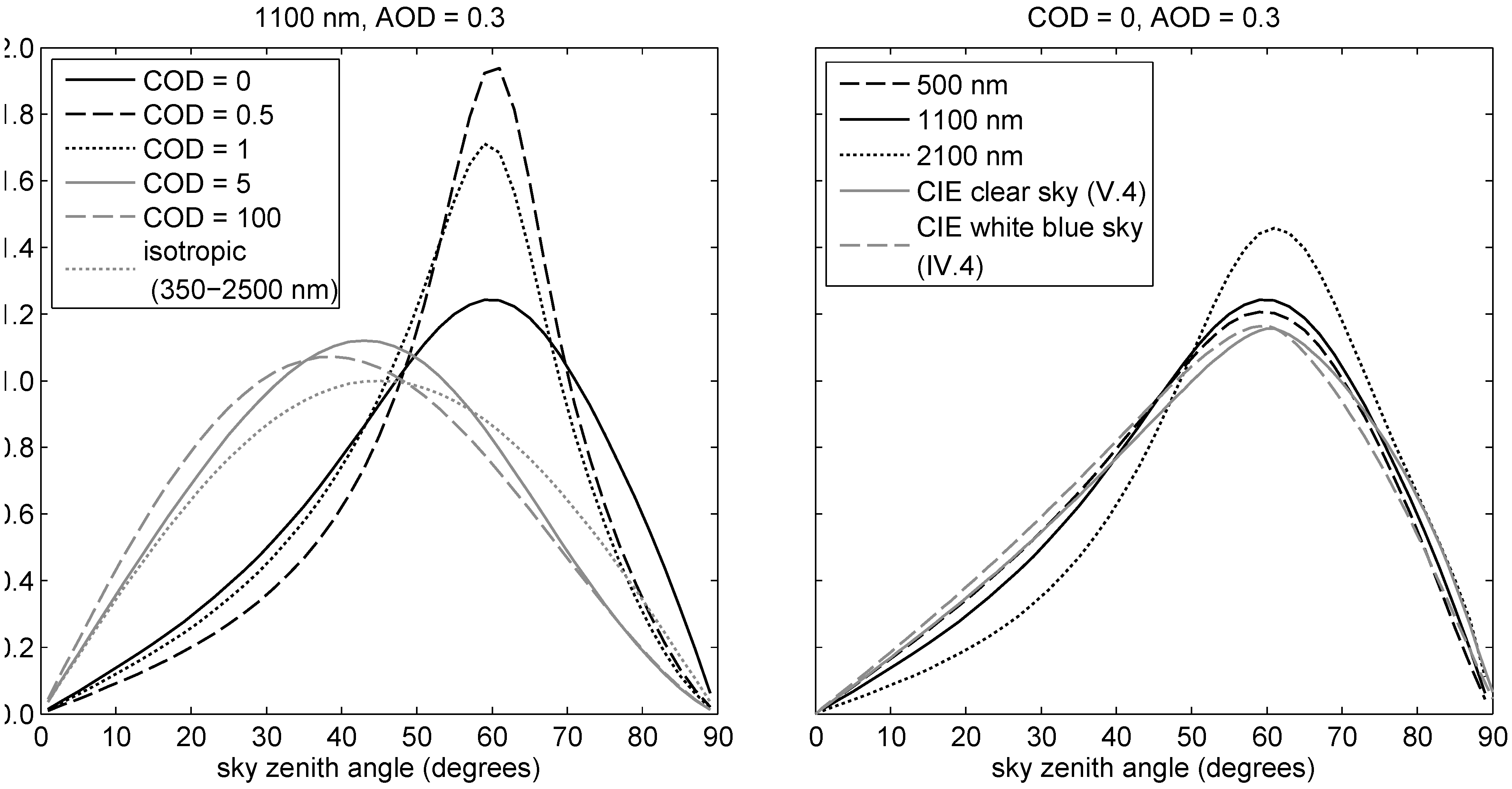
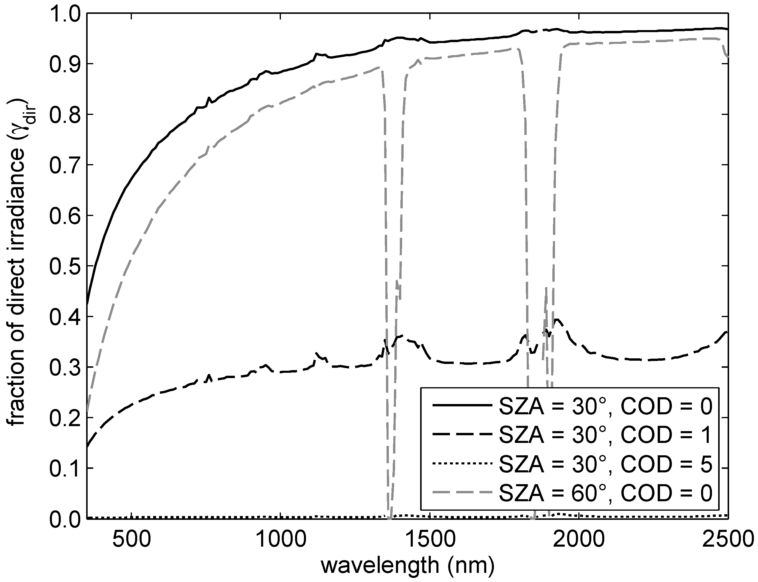
4.2. Wavelength Dependency of Fraction of Diffuse Radiance and Weight Function

Figure 2 shows fractions of direct irradiance ( γ d i r ) simulated with the atmospheric radiative transfer model SBDart for some typical mid-latitude illumination conditions and different levels of cloud optical depth (COD). For overcast skies (COD ≥ 5, black dotted line at the bottom) almost all the light is diffuse so that γ d i r is equal or close to zero for all wavelengths.
Figure 2. Fraction of direct irradiance for different values of solar zenith angle (SZA) and cloud optical depth (COD) simulated with SBDart. Simulations used fixed values for atmosphere optical depth (0.3), cloud altitude (4,000–4,400 m), water vapor content ( 2.5 g c m - 2 ) and ozone content ( 0.3 a t m c m - 1 ).
Remotesensing 01 00496 g002
Figure 3 shows the angular distributions of diffuse light projected onto a horizontal plane, simulated with SBDart and normalized as a weight function as described in Section 2.4. Curves are plotted for a solar zenith angle of 60°, aerosol optical depth of 0.3 and different cloud optical depths (left figure) and wavelengths (right figure). As a reference on the left figure, the weight function is plotted of a hypothetical isotropic distribution that takes the shape of a half sine curve (grey dotted line). Large differences exist between the different weight functions, demonstrating the importance of accounting for angular distributions of diffuse light to obtain good quality normalizations of BRDF effects in DFOV spectroscopy. To increase optical depths, the weight function first concentrates around the solar disk (COD = 0.5) and for higher values (COD > 5) it converges into a fixed distribution, with a maximum weight around the 40° sky zenith angle (grey dashed line). Different simulations confirm that for COD = 100, the weight function becomes largely independent of wavelength with the exception of the higher SWIR wavelengths (R² between weight functions at different wavelength > 0.99 from 350 to 1,340 nm and from 1,520 to 1,790 nm), solar zenith angle (R² between 10° and 80° > 0.99) and aerosol optical depth. The CS weight functions (right figure) have more articulated maxima for increasing wavelengths due to more atmospheric Rayleigh scattering in addition to the Mie scattering by clouds. The right figure in addition shows the weight functions derived for the CIE white blue sky and clear sky types as defined in [20] at a 60° SZA. The coefficient of determination between both functions ranges from 0.99 for a 10° SZA to 0.97 for a 80° SZA. These observations indicate that at least for the visible wavelengths (CIE is defined as luminance) the difference between CS and QCS reflectance factors as defined in section 2.5 will be limited.
Figure 3. Angular distribution of diffuse incident light expressed as a weight function, for different values of cloud optical depth (left figure) and wavelengths (right figure) simulated with SBDart or derived from the CIE formulations [20] for a 60° solar zenith angle.
Remotesensing 01 00496 g003

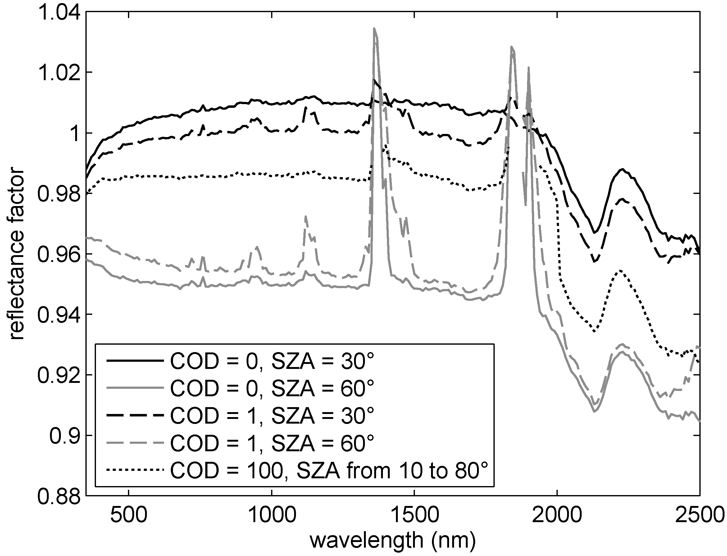
4.3. Impact of Reference Panel BRDF

Figure 4 shows the reflectance factor of a Spectralon whitepanel for different illumination conditions, calculated using Equation 5 with wavelength dependent skylight distributions (weighting factors) and fractions of direct irradiance simulated with SBDart. The target BRDF is derived from the correction factor for the non-Lambertian behavior of Spectralon material as established by [18]. The BRDF effects caused by a small cloud optical depth (COD = 1) compared to a clear sky (COD = 0), with a SZA fixed at either 30° (dashed and solid black lines) or 60° (dashed and solid grey lines) are below 1%. For high cloud thickness (COD = 100, equal for all SZAs), deviations from CS reflectance range from approximately 1% to more than 3%. For low solar azimuths (SZA = 30°), obscuration causes an underestimation of the panel CS reflectance factor, while for high solar azimuths, this effect reverses. It is thus expected that the use of a reference panel in DFOV spectroscopy will substantially contribute to BRDF effects if not corrected for. In the establishment of a time series over a span of several months, single FOV spectroscopy will also likely require corrections for reference panel BRDF unless a field protocol is adopted to measure under constant solar elevation. Whether the non-Lambertian nature of the reference panel will intensify or (partly) compensate BRDF effects of different targets will depend on the specific BRDF shape of those targets and more specifically on the dominant optical scattering process (geometric-optical or volume scattering) that determines this shape [21].
Figure 4. Reflectance factor of Spectralon whitepanel for different cloud optical depths and solar zenith angles calculated with polynomial approximations of [18].
Remotesensing 01 00496 g004

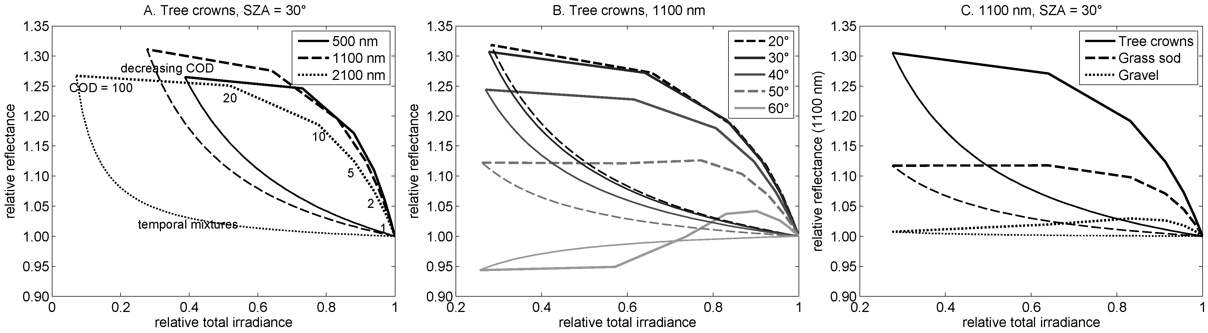
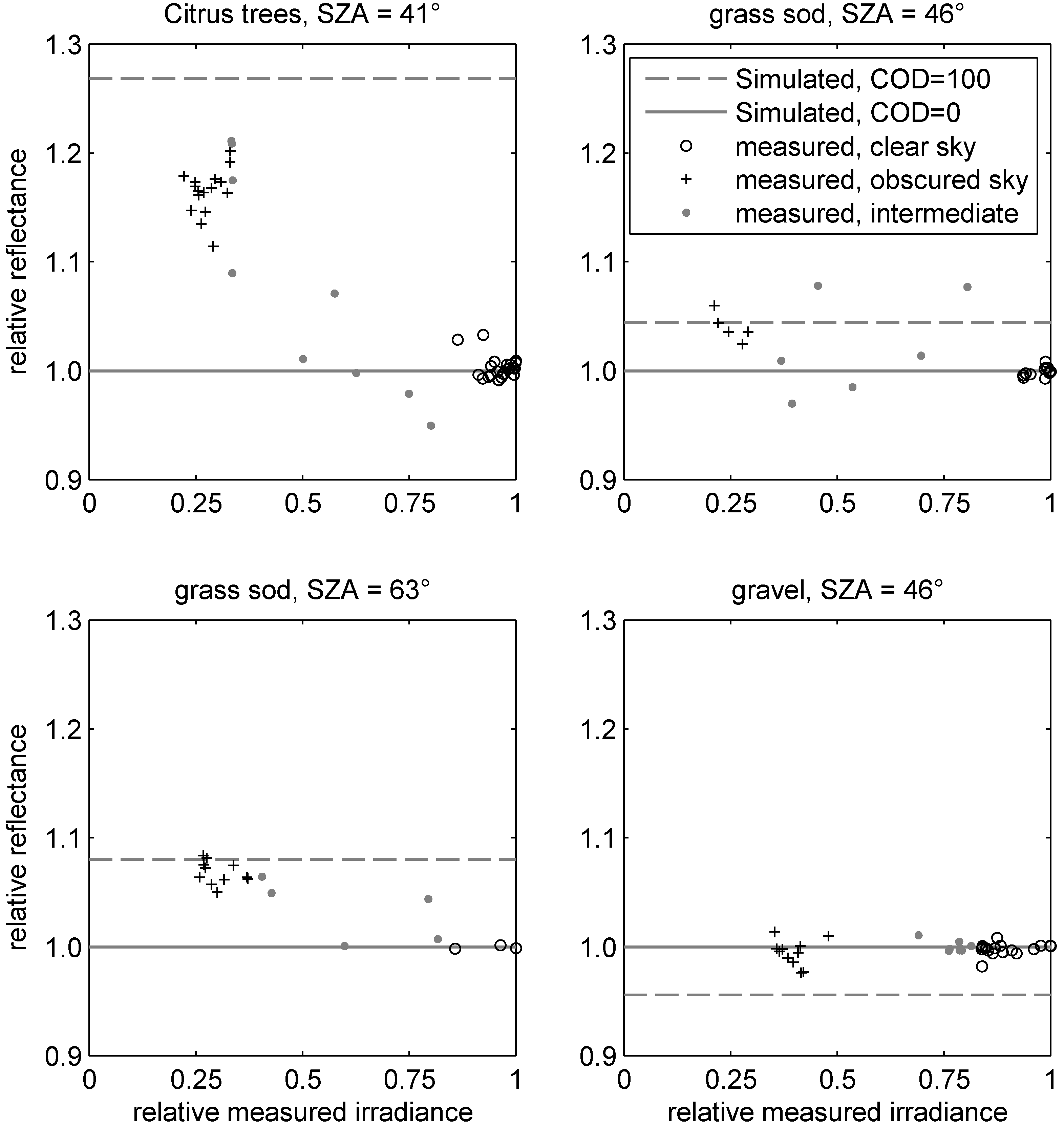
4.4. Effect of Fluctuations in COD and Irradiance During Scan Time

The normalization procedure developed in Section 2.5 relies on the measurement of total irradiance. When measuring under partly cloudy conditions, however, the optical depth of clouds obscuring the solar disk and corona and therefore also total irradiance can exhibit large fluctuations during a measurement scan. Measured total irradiance can be the result of either an almost constant illumination under intermediate cloud thickness or a mixture of high irradiance with unobscured and low irradiance with obscured conditions caused by a thick cloud layer. To assess the impact of varying illumination during a scan, effects were simulated of clouds moving before the solar disk during a short (10 s) time interval. For a 10 s scan, reflectances were calculated ranging from a clear sky (CS, COD = 0) to fully obscured sky (OS, COD = 100) for different mixture levels (α) ranging from 0% obscuration (of the scan time) to 100% obscuration. Since spectroradiometers collect radiance rather than reflectance, the result is a linear mixture of reflected radiances (L), but is non-linear with respect to reflectance factors (ρ):
ρ m e a s α ( λ ) = α L t a r C S ( λ ) + 1 - α L t a r O S ( λ ) α L r e f C S ( λ ) + 1 - α L r e f O S ( λ ) = α E C S ( λ ) ρ t a r C S ( λ ) + 1 - α E O S ( λ ) ρ t a r C S ( λ ) α E C S ( λ ) ρ r e f C S ( λ ) + 1 - α E O S ( λ ) ρ r e f C S ( λ )
with L t a r C S , L t a r O S , L r e f C S and L r e f O S the target and reference reflected spectral radiances and E C S and E O S the total spectral irradiances for both clear and obscured conditions.
Figure 5 shows the results of simulations for different combinations of wavelengths, solar elevations and targets. The X-axis shows the relative total irradiance, scaled to the maximum value (CS conditions). The Y-axis shows the reflectance relative to CS conditions and thus equals the inverse of the normalization factor ( n f ) to convert to CS conditions. Each simulation is shown as two curves forming a loop of which the thick line contains (from left to right) decreasing levels of COD and the thin line contains (from left to right) increasing fractions (α) of CS illumination. The difference between both lines is apparent for most simulations and presents a dilemma for applying a normalization based on total irradiance: if no instantaneous irradiance measurements but only the average irradiance is collected during a scan, it is not possible to discriminate scans with stable and intermediate levels of COD (between 1 and 10) from scans with strong fluctuations in COD. As a consequence the normalization factor can take any value between the upper and lower curve of a loop. A solution is restricting measurements to scans with assured stable illumination conditions (i.e., the outer edges where both curves converge) with either high (>10) or low (<1) values of COD, possibly in combination with a reduction of the scan time. The COD threshold values may change depending on target type and maximum BRDF-induced bias and values used here ascertain relative deviations on Citrus tree canopies to be below 5% (see Figure 5A). This allows field measurement scans to be subdivided into “quasi clear sky scans” and “obscured sky scans”, with a normalization applied only to the latter group. The relative flatness of the upper curves for CODs between 20 and 100 indicates an approximately constant normalization factor once cloud thickness (COD) reaches a certain level. Conversely, the steep slope of the curve for low COD values indicates that even thin (cirrus) clouds may trigger a substantial BRDF effect. The shape of the lower curves of the loops stresses the importance of stability of the illumination conditions during the scan time, as even a small mixture fraction of direct sunlight greatly impacts the relative reflectance.
Figure 5. Relative reflectance compared to clear sky reflectance simulated with pbrt and SBDart for gradually increasing cloud optical depth (thick curves) and different mixtures between clear and obscured conditions (thin curves). Simulations for (a) three different wavelengths, (b) five solar zenith angles and (c) three surface types.
Remotesensing 01 00496 g005
For most simulations, reflectance under obscured conditions is higher than under CS conditions (relative reflectance > 1). Only for tree canopies simulated with low solar elevation angles (middle figure, SZA = 60°) an inversion occurs. The BRDF shape of vegetation targets and, to a lesser extent, of rough soil surfaces (gravel) thus seems opposite to the BRDF effects of the whitepanel (Figure 4). Hence the ratio of both radiances (Equation 5) will reinforce rather than compensate the overall BRDF effect.
The differences between the loops on the three figures show that each combination of target type and solar zenith angle requires a different wavelength-dependent normalization factor. For DFOV time series this implicates that for the same type of target, throughout a measurement season different normalization factors may need to be established.

4.5. Evaluating the Decomposition of the Target BRDF

The normalization strategy developed in Section 2.5 relies on the assumption that the BRDF of a target can be split into a target specific component independent of viewing and illumination geometry and a bidirectional component that describes the behavior of a group of targets, i.e., f t a r ρ t a r d h κ t a r . A simulation was set up to evaluate the impact of this assumption on the performance of the normalization procedure. The evaluation was made for the Citrus tree canopy targets that showed the largest BRDF effects (Figure 5c). Ten iterations were set up for solar zenith angles of 30° and 60° in which subsequently each of the ten calibrated Citrus trees was used as a reference to construct a normalization factor ( n f ) as the ratio of reflectance with obscured sky (COD = 100) and clear sky (COD = 0). In each iteration the n f was used to normalize the obscured sky reflectances of the nine remaining trees to clear sky conditions. The performance of the procedure was expressed as the relative root mean square error (RRMSE) between true and normalized clear sky reflectance (Figure 6). The results show that not correcting reflectance for BRDF effects results in substantial errors between 20% and 40% for solar elevations of 30°. At an elevation of 60° the uncorrected relative errors fall below 10%. Both results corresponds to Figure 5b. Applying the n f results in an improvement for the 30° SZA simulation and a smaller improvement (except between 1400 and 2000 nm) for the 60° SZA simulation. Normalized spectra consistently have an average RRMSE below 5%. This is comparatively low considering the large variations in canopy structure and leaf reflectance present in the Citrus tree dataset (see Section 3.2 and [27]). Whether or not errors of this magnitude are acceptable will be application-dependent.
Figure 6. Relative error in reflectance of the simulated Citrus trees under cloudy conditions (COD = 100) using a clear sky reflectance (COD = 0) as a reference, simulated with pbrt and SBDart. Averages for 10 Citrus tree canopy targets and two solar zenith angles. Black curves: uncorrected reflectance, grey curves: corrected reflectance.
Remotesensing 01 00496 g006

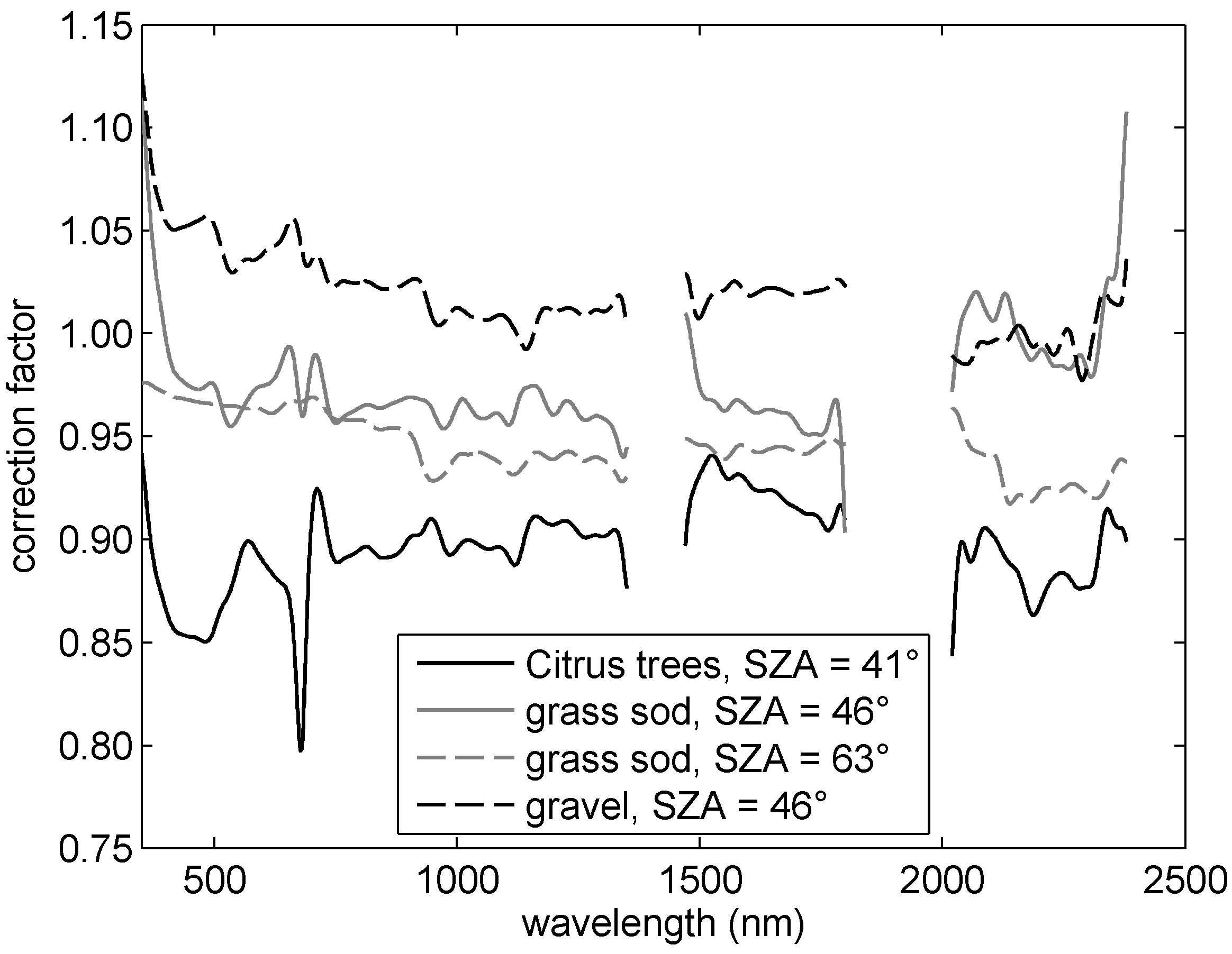
4.6. Interpretation of Measured BRDF Effects

Figure 7 shows, for four different measurement sets, the relative reflectance factor between 1,050 and 1,150 nm (around the peak NIR reflectance of vegetations) as a function of total irradiance. Reflectance factors for each figure were normalized to average reflectance under unobscured conditions. Irradiance values were normalized to the maximum total irradiance per measurement sets. Most of the points on the scatter-plots are grouped into two clusters (black dots): one for high irradiance (unobscured) and one for low irradiance (obscured). The limited number of intermediate points (grey dots) show large fluctuations. This agrees with the simulations in Section 4.4 (Figure 5) where intermediate measurements could take any position between the upper and lower curve of a loop. Most intermediate points have relative reflectances closer to 1 indicating that most of them are caused by irradiance fluctuations during the scan time.
Figure 7. Measured relative reflectance factor between 1,050 and 1,150 nm, normalized to reflectance at quasi clear sky conditions (10 percentile highest values). The X-axis shows the relative total irradiance, scaled to the highest measured value.
Remotesensing 01 00496 g007
For each measurement set a virtual model was constructed with a comparable canopy or soil structure and reflectance and simulated with PBRT (see Section 3.2) under an approximately equal illumination (solar elevation), for both clear and obscured conditions. For each simulation, a wavelength-dependent n f was derived using the procedure of Section 2.5. The n f s calculated for the same wavelength interval are drawn as horizontal dashed lines on Figure 7. For an ideal agreement between simulated and measured datasets, these line should thus pass through the centers of the point clusters for obscured conditions. The simulated n f for tree canopies is overestimated, the n f s for the grass sods under high and low solar elevations show good agreement with the measurements and the n f for the gravel surface is underestimated. Similar results were obtained for other wavelengths (results not shown here). In general both simulated and measured datasets show a similar behavior of relative reflectance as a function of relative irradiance, although the magnitude of the effects are not always equal. It can be concluded that relative differences in reflectance factor related to differences in illumination are well explained and described by the theory presented in Section 2.4 and Section 2.5. The use of synthetic n f s to correct DFOV measurements can however be questioned.

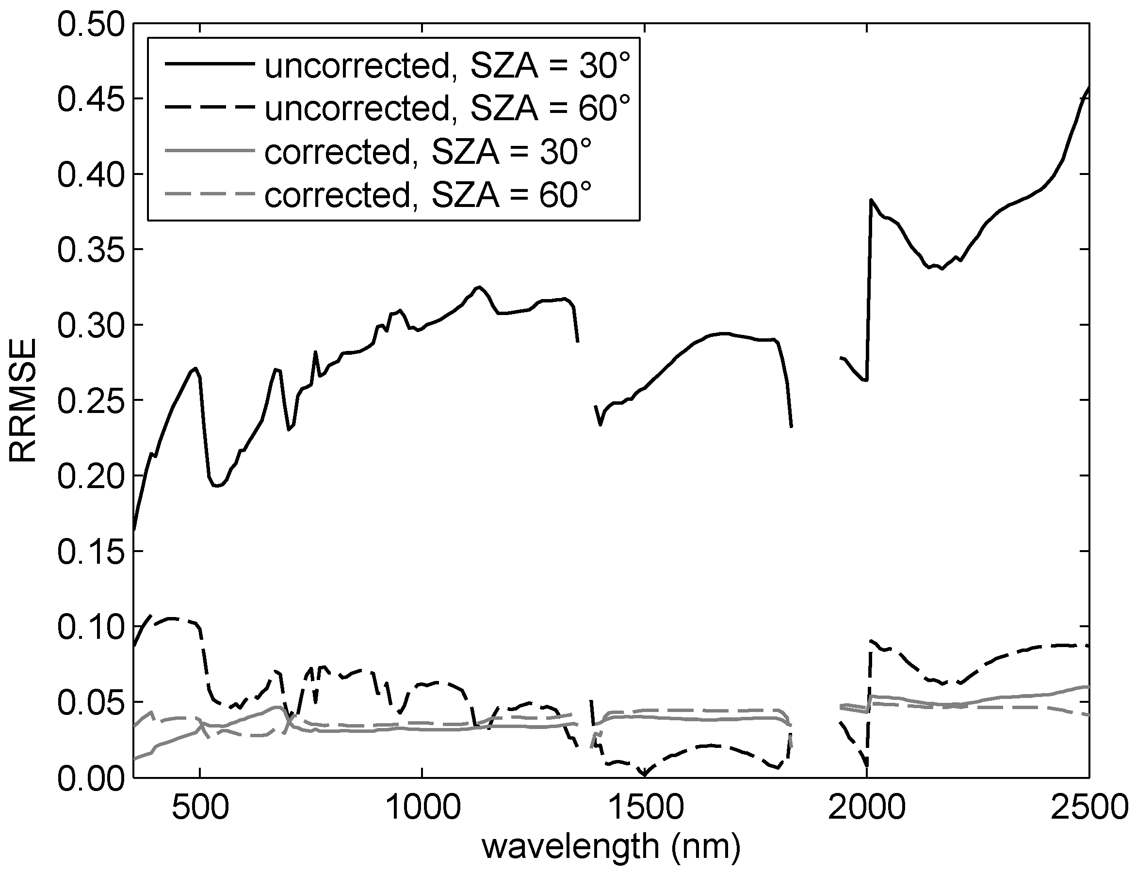
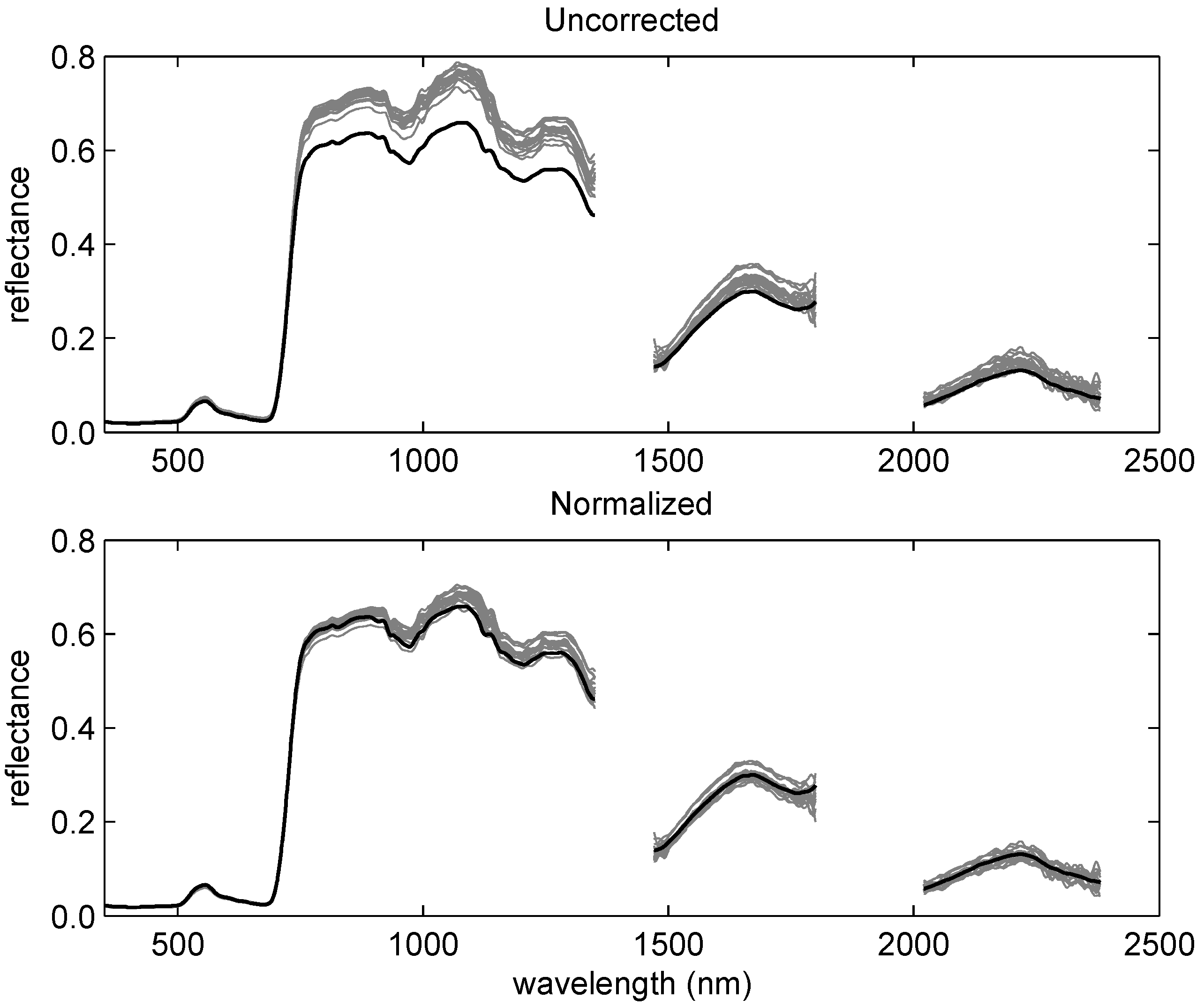
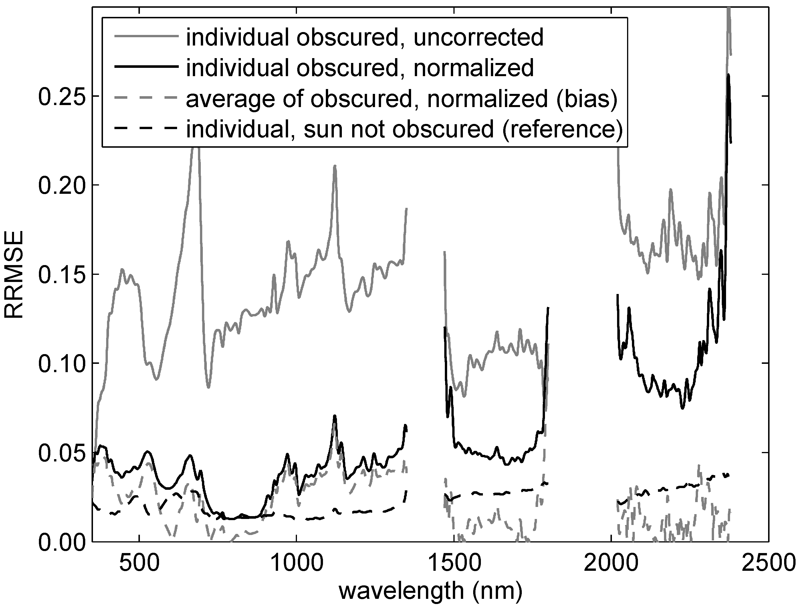
4.7. Data-Driven Normalization

The alternative to synthetic n f s is a data-driven approach in which an n f is obtained from a reference target with equal solar elevation and varying grades of cloud cover. Figure 8 shows spectral n f s obtained for the four different field-collected datasets. The n f s for each dataset were obtained as the ratios of average QCS to average OS reflectance factors, while intermediate values (>150% of lowest total irradiance and <80% of highest total irradiance) were removed to minimize irradiance fluctuations during scan time (see Section 4.4 and Section 4.6). Removed spectra accounted for less than 20% of the measurements in each dataset. As predicted from the simulation data, the values of the n f s are spectrally variant, depend on the solar elevation angle and show large differences between target types (grass sod, tree canopy, gravel). Both negative and positive values occur.
Figure 8. Normalization factors derived for four field measurements sets.
Remotesensing 01 00496 g008
A n f derived from a DFOV dataset of measured Citrus tree canopy reflectance (black solid line) was subsequently applied to normalize a second DFOV dataset of different Citrus trees (same variety and phenology) with comparable structure, measured under similar illumination conditions (difference in average SZA below 4°). Figure 9 compares measured reflectance under obscured conditions (grey lines) to the average unobscured reflectance factor (black line) for both original uncorrected and normalized data. The normalized results show a better fit over the entire spectrum although the normalized reflectance still shows a small overestimation in the NIR.
Figure 9. Reflectance factor of Citrus trees measured under obscured conditions (grey lines, individual scans) with a reference (black line, average value) measured under unobscured conditions. Top figure: uncorrected spectra. Bottom figure: after multiplication with a normalization factor.
Remotesensing 01 00496 g009
Figure 10 shows the RRMSE of the cloud obscured data compared to the unobscured data. Without normalization, relative errors range between 10% and 20%. After normalization, relative errors fall below 6% up to 1,800 nm, but reach values up to 10% for higher wavelengths. As compared to the simulations of Figure 6, the magnitude of the errors is comparable up to 1,800 nm. To separate BRDF-related bias from noise (which is not present in the simulations), the RRMSE of the average of the normalized measurements is also plotted. In this average spectrum the noise term is reduced by a factor of 4.1 (17 scans) so that it represents an upper bound to BRDF-related bias. The low values between 1,500 and 2,500 nm indicate that for the individual normalized scans (solid black line), the increased RRMSE beyond 1800 nm is no bias, but caused by a low SNR (see Figure 1) related to severely reduced irradiance. As a second reference the relative standard deviation of the unobscured (reference) measurements is plotted on Figure 10, which is consistently below 4%. It reflects the error term under quasi clear sky conditions and is attributed to electronic sensor noise, small target changes (wind) or BRDF effects due to small changes in illumination (AOD) or solar elevation during a measurement set [4].
Figure 10. Relative error in reflectance (RRMSE) of measurements under obscured conditions using unobscured measurements as a reference.
Remotesensing 01 00496 g010
For vicarious calibration, normalization to (quasi) clear sky conditions as presented here is still required. The construction of time series in field spectroscopy on the other hand can benefit from a normalization to standardized illumination conditions to separate BRDF effects due to illumination conditions (solar elevation) from changes in target reflectance, e.g., due to vegetation physiology. The same approach can therefore inverted to normalize to reflectance with a homogeneous cloud obscured sky. When the COD is sufficiently high (>5), for all wavelengths in the 400–2,500 nm region, almost all the incident light is diffuse ( γ d i r 0 ) and the weight function is almost constant (see Section 4.2) and approximately isotropic [20, 37]. The reflectance factor measured under overcast conditions will therefore offer an approximation of hemispherical-directional reflectance ( ρ h d ) with nadir viewing angle or directional-hemispherical reflectance ( ρ h d , or black-sky albedo) with zenith illumination according to the Helmholtz reciprocity principle.

5. Conclusions

The impact of reduced irradiance caused by cloud cover on the SNR of the measured reflectance factor was quantified. Results suggest that data quality standards (minimal SNR) can be converted into instrument and wavelength specific lower bounds for illumination conditions (spectral irradiance) under which DFOV spectroscopy can be deployed.
BRDF effects in DFOV measurements could be modeled and described using synthetic data in a ray tracing environment. Solar elevation, wavelength and target type (structural composition) were found to be the determinant factors affecting differences between reflectance factors under obscured and unobscured conditions, while the reference panel BRDF will often reinforce this effect.
A data-driven normalization procedure and its underlying assumption (decomposition of the BRDF into a target specific isotropic and a group specific bidirectional component) were evaluated on both synthetic and real datasets. Results indicate that most of the bias in cloud obscured measurements can be removed by applying a normalization factor obtained by from a representative target under equal illumination conditions, without the need to obtain an exact description of the bidirectional component of the target BRDF ( κ t a r ). Field protocols should avoid or remove measurements that include large irradiance fluctuations during scan time as well as measurements made with intermediate COD values corresponding to intermediate irradiance levels. Threshold values depend on the acceptable bias. Normalized spectra show low relative errors up to 1,800 nm, but at higher wavelengths, an increase in relative error was attributed to a reduced SNR. For DFOV applications requiring the full 350–2,500 nm spectrum, a larger number of scans per individual target may be required to lower the noise level. The inclusion of a BRDF normalization, in addition to an intercalibration factor shows good promise to deploy DFOV spectroscopy for physiological monitoring applications in mid-latitude climate regions where a dominance of partly cloudy and overcast skies can prevent establishment of clear sky time series. The low relative errors obtained by this combined normalization (on average 5% below 1,800 nm) may meet the requirements of physiological investigations that require the detection of trends in specific zones of the spectrum.
Prior to implementation, more testing is required under a broader range of illumination conditions with different cloud types and different targets. In addition, this method can be tested in inverse mode to normalize reflectance under standardized overcast illumination conditions that are largely independent of solar elevation. This would be advantageous for the separation of physiological changes from BRDF effects in seasonal time series of vegetated targets.

Acknowledgments

This research was funded by the Katholieke Universiteit Leuven, Biosystems Department as part of the Special Research Fund program OT04047.

Appendix

This section describes the conversion of Equation 1 into Equation 5. For nadir (n) viewing directions ( θ v = 0) the relative azimuth between viewing and illumination ( φ i - φ v ) can take arbitrary values with no influence on an object’s reflected radiance. The target reflected radiance from Equation 4 can therefore be simplified into:
L t a r n = L d i r n + L d i f n L d i r n = E t o t γ d i r f t a r θ i , 0 L d i f n = 0 2 π 0 π / 2 f t a r θ , 0 L d i f ( θ , φ i ) cos θ sin θ d θ d φ
The integral part of the last equation can be simplified by defining L d i f ¯ θ = 0 2 π L d i f θ , φ d φ , multiplying by E d i f E d i f = 1 - γ d i r E t o t E d i f and expanding the denominator as a radiometric integral so that:
L d i f n = ( 1 - γ d i r ) 0 π / 2 f t a r θ , 0 L d i f ¯ θ cos θ sin θ d θ 0 π / 2 L d i f ¯ θ cos θ sin θ d θ
This equation takes the shape of a weighted average with a weight function w defined as w ( θ i ) = L d i f ¯ θ cos θ sin θ . The same conversion can be applied to the reference radiance so that the measured reflectance can be written as Equation 5.

References

  1. Milton, E.; Schaepman, M.; Anderson, K.; Kneubühler, M.; Fox, N. Progress in field spectroscopy. In IEEE International Conference on Geoscience and Remote Sensing Symposium, IGARSS 2006, Denver, CO, USA, July 31–August 4, 2006; pp. 1966–1968.
  2. ASD Technical Guide, 3rd ed.; Analytical Spectral Devices: Boulder, CO, USA, 1999.
  3. Milton, E.; Rollin, E.; Emery, D. Advances in Environmental Remote Sensing; Wiley: Chichester, UK, 1995; pp. 9–32. [Google Scholar]
  4. Sandmeier, S.R. Acquisition of bidirectional reflectance factor data with field goniometers. Remote Sens. Environ. 2000, 73, 257–269. [Google Scholar] [CrossRef]
  5. Milton, E.; Rollin, E. Estimating the irradiance spectrum from measurements in a limited number of spectral bands. Remote Sens. Environ. 2006, 100, 348–355. [Google Scholar] [CrossRef]
  6. Anderson, K.; Milton, E.; Rollin, E. Calibration of dual-beam spectroradiometric data. Int. J. Remote S. 2006, 27, 975–986. [Google Scholar] [CrossRef]
  7. Milton, E.; Goetz, A. Atmospheric influences on field spectrometry: observed relationships between spectral irradiance and the variance in spectral reflectance. In Seventh International Symposium on Physical Measurements and Signatures in Remote Sensing, Courchevel, France, April 7-11, 1997; Vol. 1, pp. 109–114.
  8. Gilabert, M.-A.; Meliá, J. Solar angle and sky light effects on ground reflectance measurements in a citrus canopy. Remote Sens. Environ. 1993, 45, 281–293. [Google Scholar] [CrossRef]
  9. Abdou, W.A.; Helmlinger, M.C.; Conel, J.E.; Bruegge, C.J.; Pilorz, S.H.; Martonchik, J.V. Ground measurements of surface BRF and HDRF using PARABOLA III. J. Geophys. Res. 2000, 106, 967–976. [Google Scholar] [CrossRef]
  10. Sandmeier, S.; Müller, C.; Hosgood, B.; Andreoli, G. Sensitivity analysis and quality assessment of laboratory BRDF data. Remote Sens. Environ. 1998, 64, 176–191. [Google Scholar] [CrossRef]
  11. Rollin, E.; Milton, E.; Emery, D. Reference panel anisotropy and diffuse radiation - some implications for field spectroscopy. Int. J. Remote Sens. 2000, 21, 2799–2810. [Google Scholar] [CrossRef]
  12. Bruegge, C.; Chrien, N.; Haner, D. A spectralon BRF data base for MISR calibration applications. Remote Sens. Environ. 2001, 76, 354–366. [Google Scholar] [CrossRef]
  13. Michalsky, J.; Harrison, L.; Berkheiser, W. Cosine response characteristics of some radiometric and photometric sensors. Sol. Energy 1995, 54, 397–402. [Google Scholar] [CrossRef]
  14. Schott, J. Remote Sensing: The Image Chain Approach, 2th ed.; Oxford Press: New York, NY, USA, 2007. [Google Scholar]
  15. Kimes, D.; Kirchner, J. Irradiance measurement errors due to the assumption of a Lambertian reference panel. Remote Sens. Environ. 1982, 12, 141–149. [Google Scholar] [CrossRef]
  16. Gu, X.; Guyot, G. Effects of diffuse irradiance on the reflectance factor of reference panels under field conditions. Remote Sens. Environ. 1993, 45, 249–260. [Google Scholar] [CrossRef]
  17. Flasse, S.; Verstraete, M.; Pinty, B.; Bruegge, C. Modeling Spectralon’s bidirectional reflectance for in-flight calibration of Earth-orbiting sensors. In Proc. SPIE, 1993, Orlando, FL, USA, April 16, 1993.
  18. Schopfer, J. Spectrodirectional ground-based remote sensing using dual-view goniometry: field BRF retrieval and assessment of the diffuse irradiance distribution in spectrodirectional field measurements. PhD thesis, University of Zurich, Zurich, Switzerland, 2008. [Google Scholar]
  19. Platt, U.; Pfeilsticker, K.; Vollmer, M. Springer Handbook of Lasers and Optics; Springer: New York, NY, USA, 2007; pp. 1165–1203. [Google Scholar]
  20. CIE, Spatial distribution of daylight-CIE Standard General Sky; Technical Report CIE Standard S 011/E:2003; CIE Central Bureau: Vienna, Austria, 2003.
  21. Lucht, W.; Schaaf, C.; Strahler, A. An algorithm for the retrieval of albedo from space using semiempirical BRDF models. IEEE T. Geosci. Remote Sens. 2000, 38, 977–998. [Google Scholar] [CrossRef]
  22. Giavis, G.; Kambezidis, H.; Sifakis, N.; Toth, Z.; Adamopoulos, A.; Zevgolis, D. Diurnal variation of the aerosol optical depth for two distinct cases in the Athens area, Greece. Atmosph. Res. 2005, 78, 79–92. [Google Scholar] [CrossRef]
  23. Igawa, N.; Koga, Y.; Matsuzawa, T.; Nakamura, H. Models of sky radiance distribution and sky luminance distribution. Sol. Energy 2004, 77, 137–157. [Google Scholar] [CrossRef]
  24. HR-1024 User Manual, rev. 1.3 ed.; Spectra Vista Corporation: New York, NY, USA, 2008.
  25. Pharr, M.; Humphreys, G. Physically Based Rendering: From Theory to Implementation; Morgan Kaufmann: San Francisco, CA, USA, 2004. [Google Scholar]
  26. Widlowski, J.-L.; Robustelli, M.; Disney, M.; Gastellu-Etchegorry, J.-P.; Levergne, T.; Lewis, P.; North, P.; Pinty, B.; Thompson, R.; Verstraete, M. The RAMI On-line Model Checker (ROMC): A web-based benchmarking facility for canopy reflectance models. Remote Sens. Environ. 2008, 112, 1144–1150. [Google Scholar] [CrossRef] [Green Version]
  27. Stuckens, J.; Somers, B.; Delalieux, S.; Verstraeten, W.; Coppin, P. The impact of common assumptions on canopy radiative transfer simulations: A case study in Citrus orchards. J. Quant. Spectrosc. Ra. 2009, 110, 1–21. [Google Scholar] [CrossRef]
  28. Jacquemoud, S.; Baret, E.; Hanocq, J. Modeling spectral and bidirectional soil reflectance. Remote Sens. Environ. 1992, 41, 123–132. [Google Scholar] [CrossRef]
  29. Bunnik, N.J.J. The Multispectral Reflectance of Shortwave Radiation of Agricultural Crops in Relation with Their Morphological and Optical Properties. PhD Thesis, Mededelingen Landbouwhogeschool Wageningen, Wageningen, The Netherlands, 1975. [Google Scholar]
  30. Hosgood, B.; Jacquemoud, S.; Andreoli, G.; Verdebout, J.; Pedrini, A.G.S. Leaf Optical Properties EXperiment 93 (LOPEX93); Technical report; Joint Research Centre, Institute for Remote Sensing Applications, Unit for Advanced Techniques, TP 272: Ispra (VA), Italy, 1994. [Google Scholar]
  31. Somers, B.; Delalieux, S.; Verstraeten, W.; Coppin, P. A conceptual framework for the simultaneous extraction of sub-pixel spatial extent and spectral characteristics of crops. Photogramm. Eng. Remote Sens. 2009, 1, 57–68. [Google Scholar] [CrossRef]
  32. Bousquet, L.; Lachérade, S.; Jacquemoud, S.; Moya, I. Leaf BRDF measurements and model for specular and diffuse components differentiation. Remote Sens. Environ. 2005, 98, 201–211. [Google Scholar] [CrossRef]
  33. Ricchiazzi, P.; Yang, S.; Gautier, C.; Sowle, D. SBDART: A research and teaching software tool for plane-parallel radiative transfer in the Earth’s atmosphere. Bull. Am. Meteorol. Soc. 1998, 79, 2101–2114. [Google Scholar] [CrossRef]
  34. Carrer, G. Ratios of leaf reflectances in narrow wavebands as indicators of plant stress. Int. J. Remote Sens. 1994, 15, 697–704. [Google Scholar]
  35. Haboudane, D.; Miller, J.; Pattey, E.; Zacro-Tejada, P.; Strachan, I. Hyperspectral vegetation indices and novel algorithms for predicting green LAI of crop canopies: Modeling and validation in the context of precision agriculture. Remote Sens. Environ. 2004, 90, 337–352. [Google Scholar] [CrossRef]
  36. Roberts, M. Signals and Systems: Analysis of Signals Through Linear Systems; McGraw-Hill Higher Education: Whitby, Ontario, L1N 9B6, Canada, 2003. [Google Scholar]
  37. Schaepman-Strub, G.; Schaepman, M.; Painter, T.; Dangel, S.; Martonchik, J. Reflectance quantities in optical remote sensing - definitions and case studies. Remote Sens. Environ. 2006, 103, 27–42. [Google Scholar] [CrossRef]

